Multi-level Modelling Under Informative Sampling
Danny Pfeffermann, Fernando Moura, Pedro Nascimento Silva
Abstract
We consider a model dependent approach for multi-level modelling that accounts for informative probability sampling, and compare it with the use of probability weighting as proposed by Pfeffermann et al. (1998a). The new modelling approach consists of first extracting the hierarchical model holding for the sample data as a function of the corresponding population model and the first and higher level sample selection probabilities, and then fitting the resulting sample model using Bayesian methods. An important implication of the use of this approach is that the sample selection probabilities feature in the analysis as additional outcome values that strengthen the estimators. A simulation experiment is carried out in order to study and compare the performance of the two approaches. The simulation study indicates that both approaches perform generally equally well in terms of point estimation, but the model dependent approach yields confidence (credibility) intervals with better coverage properties. A robustness simulation study is performed, which allows to assess the impact of misspecification of the models assumed for the sample selection probabilities under informative sampling schemes.
MULTI-LEVEL MODELLING UNDER INFORMATIVE SAMPLING
By DANNY PFEFFERMANN
Department of Statistics, Hebrew University, Jerusalem, 91905 Israel, Southampton Statistical Sciences Research Institute, Southampton SO17 1BJ, UK
FERNANDO MOURA
Department of Statistical methods, Federal University of Rio de Janeiro, 21945-970, Brazil (*)
PEDRO NASCIMENTO SILVA
Escola Nacional de Ciencias Estatisticas, Rio de Janeiro, 20231-050, Brazil
SUMMARY
We consider a model dependent approach for multi-level modelling that accounts for informative probability sampling, and compare it with the use of probability weighting as proposed by Pfeffermann et al. (1998a). The new modelling approach consists of first extracting the hierarchical model holding for the sample data as a function of the corresponding population model and the first and higher level sample selection probabilities, and then fitting the resulting sample model using Bayesian methods. An important implication of the use of this approach is that the sample selection probabilities feature in the analysis as additional outcome values that strengthen the estimators. A simulation experiment is carried out in order to study and compare the performance of the two approaches. The simulation study indicates that both approaches perform generally equally well in terms of point estimation, but the model dependent approach yields confidence (credibility) intervals with better coverage properties. A robustness simulation study is performed, which allows to assess the impact of misspecification of the models assumed for the sample selection probabilities under informative sampling schemes.
Some key words: Confidence (Credibility) intervals, MCMC, Probability weighting, Small area estimation, Sample distribution
1. INTRODUCTION
Multi-level (mixed linear) models are frequently used in the social and medical sciences for modelling hierarchically clustered populations. Classical theory underlying the use of these models assumes implicitly that either all the clusters at all the levels are represented in the sample, or that they are sampled completely at random. This assumption may not hold in a typical sample survey where the clusters and/or the final sampling units are often sampled with unequal selection probabilities. When the sampling probabilities are related to the values of the outcome variable even when conditioning on the model covariates, the sampling process becomes informative and the model holding for the sample data is then different from the population model. Ignoring the sampling process in such cases may yield biased point estimators and distort the analysis.
As an example, consider an education study of pupils’ proficiency with schools as the second level units and pupils as first level units, and suppose that the schools are sampled with probabilities proportional to their sizes. Under this (commonly used) sampling scheme the sample of schools will tend to contain mostly large schools, and if the size of the school is related to the pupils’ proficiency but the size is not included among the model covariates, the schools in the sample will not represent correctly the schools in the population and therefore follow a different model. A situation where the size of the school is related to the pupils’ proficiency is when the larger schools are mostly located in poor areas with low proficiency. As implicitly suggested by this example, a possible way of handling the problem of informative sampling is by including among the model covariates all the design variables that define the selection probabilities at the various levels. However, this paradigm is often not practical. First, not all the design variables used for the sample selection may be known or accessible to the analyst, or that there may be too many of them, making the fitting and validation of such models formidable. Second, by including the design variables among the model covariates, the resulting model may no longer be of scientific interest. This is not necessarily a problem when the fitting of the model is for prediction purposes, but is clearly not acceptable when the purpose of the analysis is to study the structural relationship between the outcome variable and covariates of interest.
asymptotic arguments but it was shown to perform well in a simulation study also with moderate sample sizes. Nonetheless, the use of the sampling weights (inverse of the sample inclusion probabilities) for bias correction has four important limitations:
1- The variances of the weighted estimators are generally larger than the variances of the corresponding unweighted estimators.
2- Inference is restricted primarily to point estimation. Probabilistic statements require asymptotic normality assumptions. The exact distribution of weighted point estimators is generally unknown.
3- The use of the sampling weights does not permit in general to condition on the selected sample of clusters (second and higher level units), or values of the model covariates.
4- It is not clear how to predict with this approach second and higher level random effects under informative sampling; for example, how to predict the mean school proficiency for schools not represented in the sample. Notice that under informative sampling, the schools not represented in the sample also form an ‘informative sample’ that behaves differently from the schools in the population. We mention in this respect that multi-level models are in common use for Small Area Estimation problems, where the prediction of the higher level (area) means is the primary objective of the model fitting.
In this article we consider a model dependent approach for multi-level modelling under informative sampling and compare it to the use of probability weighting. The idea behind the use of the modelling approach is to first extract the hierarchical model holding for the sample data as a function of the corresponding population model and the conditional expectations of the first and higher level sample selection probabilities given the observed data and the model random effects, and then fit the sample model using Bayesian methods. An important implication of the use of this approach is that the sample selection probabilities feature into the analysis as additional outcome values that strengthen the estimators. Evidently, if the sample model is specified correctly, the use of this approach overcomes the limitations underlying the use of probability weighting mentioned above. However, as illustrated and discussed later, misspecification of the models assumed for the sample selection probabilities may bias some of the model parameter estimators. (A similar problem is shown to underlie the use of probability weighting when the sample selection probabilities are unknown, like as in nonresponse.)
We consider for convenience a two-level model and apply the full Bayesian paradigm by use of Markov Chain Monte Carlo (MCMC) simulations, but the approach can be extended to higher level models and different inference procedures. The empirical study is restricted to simulated data from known models, which enables us to study the bias of the various estimators and the performance of the corresponding confidence (credibility) intervals.
In Section 2 we define the population model and extract the corresponding sample model for a general class of sampling designs underlying the present study. Section 3 outlines the probability weighting approach proposed in Pfeffermann et al. (1998a). Section 4 describes the simulation experiment designed for studying and comparing the performance of the two approaches, and develops the corresponding sample model. Section 5 describes the various steps in the application of the MCMC algorithm for fitting the sample model. The results of the simulation study are presented and discussed in Section 6. Section 7 presents the results of a robustness simulation study carried out for assessing the performance of the two approaches when the sampling schemes are informative but the models assumed for the sample selection probabilities are misspecified. We conclude in section 8 by summarizing the main conclusions from the present study.
2. POPULATION MODEL, SAMPLING DESIGN AND SAMPLE MODEL
2.1Population Model
In this article we consider the following two-level hierarchical model:
First level: yij|E0i E0ixij’EHij ;Hij ~ N(0,V2), j 1...Mi (1)
Second level: i zi’ ui ;ui ~N(0, u2),i 1...N
0 J V
E (2)
This model is often referred to in the literature as the random intercept regression model, and it contains as unknown hyper-parameters the vectors of coefficients E,
J
, and the firstand second level variances 2
V and 2
u
V . Note that the intercepts are modelled as linear
functions of known regressor values,
z
i. In the simulation experiment described in Section 4we refer to the outcome
y
ij as the test score of pupil j in schooli
,x
ij defines the sex, agegeographical regions. The second level random effect
u
i accounts for the variation of theintercept E0i, not explained by the regressors
z
i.2.2 Sampling Design
We assume a two stage sampling process. In the first stage,
n
N
second level units (say, schools) are selected with probabilities Si Pr(is) that may be correlated with therandom effects
u
i. In the second stage,m
i first level units (say, pupils) are sampled fromsecond level unit
i
selected in the first stage with probabilities Sj|i Pr(jsi|is) that maybe correlated with the residuals
H
ij. Notice that the sampling of the first level units maycorrespond to a response process, in which case the probabilities Sj i| define the (unknown)
response probabilities. As seen below, the case of unknown response probabilities is handled under the model dependent approach by modelling the conditional expectation of these probabilities given the observed data (see also Section 7). In Section 4 we elaborate on the sampling procedures used for the simulation study.
2.3 The Sample model
In what follows we denote by ( , ,’ 2)
0 E V
E
Ti i and O (J ,’Vu2) the respective first and
second level parameters of the population model. Following Pfeffermann et al. (1998b), the corresponding two-level sample model is,
) , | ( ) , | ( ) , , | ( ) , , | ( ) , | ( | | i ij i j p i ij ij p i ij ij i j p i i ij ij i ij ij i
s E x
x y f x y E s j x y f x y f T S T T S T
T (3)
) , | ( ) , | ( ) , , | ( ) , , | ( ) , |
( 0 0
0
0 S O
O E O E S O E O E i i p i i p i i i p i i i i
s E z
z f z E s i z f z
f (4)
where si defines the first level sample from second level unit i, s defines the second level
sample and fp() and fs() are the population and sample distributions with expectations
) (
p
E and Es() respectively.
(1999, 2003) for discussion and examples. The corresponding expressions under the sampling schemes considered for the simulation study of this article are presented in Section 4.
3. PROBABILITY WEIGHTED (DESIGN BASED) APPROACH
In this section we describe briefly the weighting procedure developed by Pfeffermann et al. (1998a). We restrict for convenience to the population model defined by (1) and (2) that contains a single second level random effect E0i. Suppose first that all the population units
are surveyed and denote by ypi ( ...yi1 yiMi)’ and Tpi ( ...t ti1 iMi) ’ the data measured for
second level unit i of size Mi, where tij (xij ,’zi’)’. Denoting also epi ( ...e ei1 iMi) ’, where
) ( ij i
ij u
e H , 2 2
V V I J
Vi u , where J and I define the unit matrix and the identity matrix
of order Mi respectively and G’ (E ,’J’), the ‘census model’ defined by (1) and (2) can be
written alternatively as,
pi pi pi
y T G e ; epi ~ (0, )N Vi , i 1...N, (E e epi pk’) 0 for i kz (5)
A commonly used procedure for estimating the vector coefficients G and the variances )’
,
( 2 2
V V
M u is the iterative generalized least squares (IGLS) algorithm, developed by
Goldstein (1986). The algorithm consists of iterating between the estimation of G for ‘given’
M, and the estimation of M for ‘given’ G , with the ‘given’ values defined by the estimates obtained on the previous iteration. The two sets of estimators are the corresponding generalized least square estimators (considering the ‘given’ values as ‘true’ ), where the observed values of the dependent variable for the estimation of G are the vectors { ,y ipi 1... }N , and the ‘observed’ values of the dependent variable for the estimation of M
on the rth iteration are the elements of the matrices
( ) ( ) ( )
ˆ ˆ ˆ
{ ( r ) ( r )( r ) ’, 1... }
i i i i i
D G y T G y T G i N , written as a vector. Notice that for known G ,
) (G
i
D has expectation Vi and that for normal error terms (ui,Hij), the variances and
covariances of the elements of Di(G) are known functions of M; see Anderson (1973) for
the corresponding expressions. The rth iteration of the IGLS yields therefore the estimators,
( ) ( ) 1 ( )
ˆr [Qr ] yr
G
; Mˆ( )r [R( )r ] 1d( )r
, r 1,2,... (6)
with appropriate definitions of the matrices Q( )r ,R( )r and the vectors y( )r ,d( )r ; see
ordinary least squares (OLS), so that the estimators Mˆ(r) use the estimators Gˆ(r), whereas the
estimators Gˆ(r) use the estimators ˆ(r1)
M , r 1,2,...Under some regularity conditions the IGLS estimators converge to the ‘census’ maximum likelihood estimators (MLE) (GˆC,MˆC) as
f o
r . (The census MLE are the MLE based on all the population data).
Suppose now that data are available for only a probability sample of second and first level units as defined in Section 2.2. The weighting procedure developed by Pfeffermann et al.
(1998a) consists of writing the matrices Q( )r ,R( )r and the vectors y( )r ,d( )r in iteration r as
sums over second level units i and first level units j, and replacing each population sum by the corresponding weighted sum of the sample units, with the weights defined by the inverse of the respective selection probabilities. Denoting the second level weights by wi 1/Si ,
and the first level weights by wj|i 1/Sj|i, and using the generic notations i and ij to
define second and first level expressions respectively, the procedure consists of replacing,
¦
N
i 1 i l
¦
n
i1wi i ;
¦
iM
j 1 ij l
¦
i
m
j 1wj|i ij (7)
Notice that each second level expression i is again a sum of the form
¦
iM
j 1 ij . It is shown
in Pfeffermann et al. (1998a) that under standard conditions the estimators Gˆ and PW Mˆ PW
obtained at the end of the iterations are consistent for the census estimators (GˆC,MˆC) under
the randomization (repeated sampling) distribution, with the latter estimators being consistent for (G, ) under the model. The consistency of I Mˆ requires that both PW n and mi tend to
infinity, but appropriate scaling of the weights wj|i controls the bias of these estimators for
small mi. A simple scaling method used in the simulation experiment of the present article is
to replace wj|i by | /( 1 | / i) m
j ji
i
j w m
w i
¦
.4. MONTE-CARLO SIMULATION EXPERIMENT
study). The target outcome values in that study were the proficiency scores of M=14,831
pupils, learning in N=392 schools, located in 3 different regions. In what follows we use ‘schools’ to define the second level units and ‘pupils’ to define the first level units. The simulation experiment consists of generating 400 populations from the model defined by (1) and (2) and selecting four samples from each population using four different sampling schemes. The various stages of the simulation experiment are described in Sections 4.1 to 4.4.
4.1 Generation of Population Values
The population values were generated in 5 steps:
Step 1 - Generate school random intercept terms from the model (Equation 2),
i i i i i
i J J J u z J u
E0 0 1Region1 2Region2 ’ ; ~ (0, 2)
u
i N
u V , i 1...392,
independently between schools. The numerical values of the J - coefficients and 2
u
V are listed in the tables of Section 6. The variables Region1i and Region2i are dummy variables
defining three school regions. The number of schools in the three regions is approximately the same.
Step 2- Generate school sizes Mi from the lognormal distribution,
] , ’
[ ~ )
log( 2
0
3 i M
i
i N z
M D D E V , with zi defined as above and D0 9.25,D1 0.31,
2 0.62
D , D3 0.045 and 2 0.050
M
V . The use of these parameter values yields school sizes with a similar distribution to the sizes of the schools in the BEE study.
Step 3- Set explanatory variables values xij for the Mi students in school i by sampling at
random with replacement Mi vectors of explanatory variables from the corresponding BEE
data in the region containing that school. The explanatory variables are dummy variables defining Sex (1 for females), Age1 (1 for age 15-16), Age2 (1 for age 17 and older) and
Parents education (1 for pupils with at least one parent having an academic degree).
Step 4 - Generate proficiency score for student j of school i using the model (Equation 1),
) , 0 ( ~ ; ’
2
1 2
0 4
3 2
1
0 E E E E H E E H H V
E Sex Age Age Parents x N
yij i ij ij ij ij ij i ij ij ij
The numerical values of the E- coefficients and 2
In order to allow for informative sampling (response) of pupils, we stratified the pupils within each school into 3 strata based on propensity scores generated as follows:
Step 5 – Generate propensity scores ; ~ (0, 2) 1
0 by ] ] N V
b
pij ij ij ij where b0 1.60,
1
b 0.0056 and 2
V 0.034. Strata membership has been assigned by setting
1
1 ( 1) if
ij ij
O stratum p c, Oij 2 (stratum2) if c1d pij c2,Oij 3(stratum3)if pij tc2,
with c1 1.76 and c2 2.16.
4.2Sampling Schemes
We consider two different methods for the sampling of schools and two different methods for the sampling (response) of pupils within the selected schools, defining a total of 4 different two-stage sampling schemes. Schools were selected using either Method A1- simple random sampling without replacement (SRSWOR) or Method A2- probability proportional to size (PPS), using Sampford (1967) method. Note that Method A2 is informative since the sizes Mi depend on the interceptsE0i (Step 2). Students within the selected schools were
sampled either by Method B1- SRSWOR or Method B2- disproportionate stratified sampling with the strata defined by the strata membership indicators Oij (three strata, Step 5). Method
B2 is informative since the strata indicators are defined based on the propensity scores pij,
which depend on the proficiency scores yij (Step 5). One sample of 50 schools and 12 pupils
from each selected school was drawn from each population using each of the 4 sampling schemes. For the stratified sample selection (Method B2) we sampled 3 pupils from Stratum 1, 4 pupils from Stratum 2 and 5 pupils from Stratum 3, yielding mean sample selection probabilities (over schools) of about 0.08 in stratum 1, 0.04 in stratum 2 and 0.14 in stratum 3.
4.3. Sample models under sampling methods A2 and B2
¦
3 1
| | , , ) Pr( | , , ) Pr( | , , )
( ji ij ij i i ij ij i k ik ij ij ij i
p y x j s y x q O k y x
E S T T T
=q1iA1(yij)q2i[A2(yij)A1(yij)]q3i[1A2(yij)] (8)
where si denotes as before the sample of pupils in school ,i qki Pr(jsi |Oij k) is the
sampling fraction in stratum k of school i, k=1,2,3 and A yk( ) Pr(ij pij c y xk| , , )ij ij Ti
0 1
[(ck b b yij) /V ]
) , where ) defines the cumulative normal distribution and c1 and c2 are the cut-off values defining the strata membership (Step 5 in Section 4.1).
The expectation in the denominator of (3) is obtained by following similar steps using the conditional density f(pij| xij,Ti). We find,
¦ 3 1
| | , ) Pr( | , )
( ji ij i k ik ij ij i
p x q O k x
E S T T
= q1iB1[P(yij)]q2i{B2[P(yij)]B1[P(yij)]}q3i{1B2[P(yij)]}, (9)
) , | ( ’ )
(yij E0i xij E Ep yij xij Ti
P ;
¸¸ ¸ ¹ · ¨¨ ¨ © § ) 2 2 1 2 1
0 ( )
) , | Pr( )] ( [ V V P T P b y b b c x c p y
B k ij
i ij k ij ij k .
The expectations featuring in the numerator and the denominator of the second level sample model (Equation 4), under the sampling method A2 are,
2 *
0 3 0
( | , , ) exp[ ’ ]
2
M
p i i i i i
E S E z O #C D z D E V (10)
2 2 2
* 3
3
( | , ) exp[ ’ ]
2
u M
p i i i i
E S z O #C D z D Jz D V V , (11)
using familiar properties of the lognormal distribution used to generate the school sizes and
the approximation, i *
i i
M
n C M
NM
S # , where
¦
N i i M N M 1
1 is the population mean of the
school sizes. Notice that the constant C* cancels out in the numerator and denominator of (4).
5. ESTIMATION OF MODEL PARAMETERS BY MARKOV CHAIN MONTE CARLO (MCMC) SIMULATION
The MCMC algorithm consists of sampling alternately from the conditional posterior distribution of each of the unknown parameters, given the data and the remaining parameters. We used for the present study the version 1.4 of the WinBUGS program, (Spiegelhalter et al.
15000 values as ‘burn in’ . Let Y { ;y iij 1... ,n j 1... }mi , O { ;O iij 1... ,n j 1... }mi and
{ ;i 1... }
M M i n denote respectively the observed y -values, the corresponding strata
membership indicators and the school sizes in the sample. The observed data consist therefore of the triple Dobs=(Y,O,M).
In what follows we use the transformations Kk (ck b0) /V , k 1, 2, K3 ( /b1 V ),
such that the probabilities Ak(yij) and Bk[P(yij)] in (8) and (9) can be written as,
) (
)
( ij k 3 ij
k y y
A )K K and ¸¸
¹ · ¨ ¨ © §
) 2 2
3 3 1 ) ( )] ( [ V K P K K
P k ij ij
k
y y
B . Notice that the K-coefficients
are considered as unknown parameters in the estimation process, implying that the cut-off values ck, the variance 2
V and the b-coefficients used to define the sampling strata in Step 5 are also considered as unknown.
The joint distribution of the observations Dobs, the parameters ( , , 2, 2)
0 E V V
E i u indexing
the population model and the additional parameters ( , , 2 )
M
V D
K indexing the sample model can be written as,
) , , , , , }, { ,
( 2 2 2
0i u M
obs
s D
f E EK D V V V
) , , , | ( ) , | ( Pr ) , , , , | ( 2 0 1 1 2
0 s i i u
n
i n
j fs yij xij Ei EK V s Oij yij K f E z J D V
) ( ). ( ). ( ). ( ). ( ). ( ). ( ). , , , |
( 2 2 2 2
0i M u M
i i
s M z p p p p p p p
f E D V E J K D V V V
u (12)
where 3
1
Pr( | , )
Pr ( | , ) Pr( | , , ) , 1, 2,3
Pr( | , )
ki ij ij
s ij ij ij ij i
ki ij ij
l
q O k y
O k y O k y j s k
q O l y
K K K K !
¦
.The sample distribution ( | , , , , 2) 0 E K V"
E i ij ij
s y x
f is defined by (3), with the expectations
appearing in the numerator and the denominator defined by (8) and (9) as functions of the
unknown K-coefficients defined above. The sample distribution ( | , , , 2)
0i i u
s z
f E J D V is
defined by (4), with the expectations appearing in the numerator and the denominator defined by (10) and (11). Here again, the D-coefficients and the variance 2
M
V are additional unknown parameters. The probabilities Pr(Oij k y x| , , )ij ij Ti are defined in (8), and after the
) ( ) , | 1
Pr(Oij yij K A1 yij ,Pr(Oij 2|yij,K) A2(yij)A1(yij),
) ( 1 ) , | 3
Pr(Oij yij K A2 yij (13)
The sample distribution of the school sizes is obtained similarly to (4) as,
) , , , | ( ) , , , | ( ) , , , , | ( ) , , , | ( 2 0 2 0 2 0 2 0 M i i i p M i i i p M i i i i p M i i i s z E z M f z M E z M f V D E S V D E V D E S V D
E . (14)
By Pfeffermann et al. (1998b), the conditional density in (14) under the sampling method A2 is lognormal; )] , ’ [ ] , , , | )
[log( 2 2
0 3 2
0i M i i M M
i i
s M z N z
f E D V D D E V V . (15)
Note that the only difference between the population distribution and the sample distribution is in this case the addition of the term 2
M
V to the mean.
The conditional posterior distributions of the various parameters given the data and the remaining parameter values, required for the application of the MCMC simulation, are obtained from the joint distribution ( ,{ }, , , , 2, 2, 2 )
M u
obs
s D
f E E K D V V# V
0i defined in (12).
Following are the posterior distribution of { }E0i and each of the vector coefficients and
variances, using the generic notation ‘Rest’ to denote the data and the remaining parameters. The notation p() is used to denote the corresponding prior distributions defined below.
n i z f z f x y f f i m j u i i s M i i s i ij ij s
i |Rest) ( | , , , , ) ( | , , , ) ( | , , , ,) 1...
( 1 2 0 2 0 2 0
0 v
$ E E KV E D V E J D VE % i M (16a)
&'& v n i mj s ij ij i
i p x y f f 1 1 2
0, , , ) ( )
, | ( ) Rest |
(E E E K V( E (16b)
) v ni s i i u
p z f f 1 2
0 | , , , ) ( )
( )
Rest |
(J E J D V J (16c)
* v ni s i i M
p z f f 1 2
0, , ) ( )
, | ( ) Rest |
(D Mi E D V D (16d)
+'+ v ni m
j s ij ij i s ij ij
i p y O x y f f 1 1 2
0 , , , )Pr ( | , ) ( )
, | ( ) Rest |
(K E E K V, K K (16e)
-'-v ni m
j s ij ij i
i p x y f f 1 1 2 2 0
2 |Rest) ( | , , , , ) ( )
(V. E E K V. V. (16f)
/ v ni s i i u u
u f z p
f
1
2 2 0
2 |Rest) ( | , , , ) ( )
(V E J D V V (16g)
0 v ni s i i M M
M f z p
f
1
2 2 0
2 |Rest) ( | , , , ) ( )
The prior distributions used in the present study are,
] 10 , 6
4
,
0 [ )
( N
p E , ,106 ]
3
,
0 [ )
( N
p J , ,103 ]
4
,
0 [ )
( N
p D , ,103 ]
3
,
0 [ )
( N
pK
) 10 , 0 ( )
( U 3
p V1 , p( ) U(0,10)
M
V , p( ) U(1,103)
u
V ; (17)
where U(a,b) defines the Uniform distribution with parameters a and b. As can be seen, all the prior distributions are very ‘flat’ . See the Comment at the end of this section regarding the
choice of the prior distribution for 2
u
V .
6. SIMULATION RESULTS
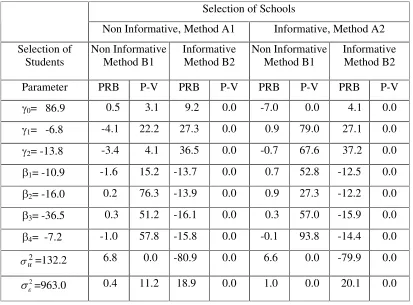
The results of the simulation study are summarized in Tables 1-3. They are based on 500 replications, each consisting of generating a new population and selecting one sample of 50 schools and 12 pupils from each selected school by each of the four sampling methods described in Section 4.2. Table 1 shows the results obtained when ignoring the sample selection schemes and fitting the population model. These results serve as benchmarks for assessing the performance of the two approaches considered in this article for dealing with the effects of informative sampling. The p-values (P-V) in the table refer to the conventional
t-tests of bias, with the standard deviation (SD) of the mean estimates computed as (1/ 500 ) times the empirical SD of the estimates over the 500 replications. The parameter estimates in a given replication are the empirical means of 5000observations drawn from the posterior distribution of each of the parameters under the population model (ignoring the sample selection schemes), after discarding the first 15000values as ‘burn in’ .
Insert Table 1 about here
The results in Table 1 illustrate the kind of biases that can be encountered when ignoring an informative sample selection scheme. In the present experiment, informative sampling (response) of pupils within the schools (Method B2) has a much stronger biasing effect than informative selection of schools (Method A2). In particular, very large relative biases are
obtained for the estimators of the ’ between schools’ variance, 2
u
variances 2 and 2
u 2
V V under non-informative sampling (response) of pupils but informative selection of schools, but as mentioned above, the biases are much smaller in this case. When both the selection of schools and the sampling (response) of pupils are noninformative, all the percent relative biases are very small and nonsignificant, except for the estimator of 2
u
V . We discuss the problem with the estimation of 2
u
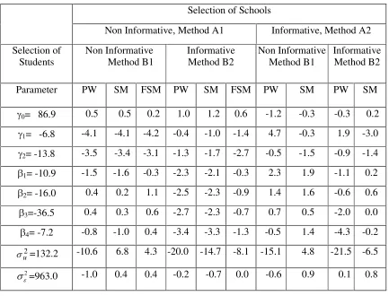
V in the comment at the end of this section. Table 2 shows the percent relative biases obtained under the two approaches that account for the sample selection and discussed in Sections 3 (probability weighting), and in Section 4 (use of the sample model). For the case of noninformative selection of schools (Method A1) and the use of the sample model, we show the results obtained when including among the model equations the equation defining the population distribution of the school sizes (Step2, Section 4.1), and also the results obtained without that equation. We refer to the first model as the ‘full’ sample model (FSM) and to the second model as simply the sample model (SM). Notice in this respect that the school selection probabilities,Si, are proportional to the school
sizes Mi, with the latter providing additional information on the random interceptsE0i, and
hence on the vector coefficient J and the variance 2
u
V indexing the distribution of the intercepts, irrespective of the sampling scheme used to select the schools. This additional information is ‘automatically’ accounted for in the case of informative selection of schools (method A2) via the corresponding sample model (Equation 16a).
Insert Table 2 about here
The biases in Table 2 are seen to be generally much smaller than the biases in Table 1, particularly under Method B2, but large (and statistically significant) biases still persist in the
estimation of 2
u
V under both methods. However, the biases are in this case much smaller when using the sample model compared to the use of probability weighting. All the other biases are in most cases statistically insignificant (the p-values are not shown in the table),
except for the biases in the estimation of 2
3
V and Jo that are occasionally significant. The
latter biases, however, are small. As expected, the use of the full sample model (FSM) that includes the model holding for the school sizes reduces some of the biases obtained under non-informative selection of schools with the use of the sample model (SM) that ignores this relationship, particularly in the estimation of 2
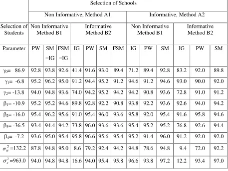
Table 3 shows the empirical percentage coverage of nominal 95% confidence (credibility) intervals (C.I.) for the model parameters, as obtained by ignoring the sampling process (IG) and by use of probability weighting (PW) and the sample models. The PW C.I. are the conventional C.I. obtained by approximating the distribution of the point estimators by the normal distribution. The randomization variances have been estimated using the sandwich-estimators developed in Pfeffermann et al. (1998a). When using the sample models or when ignoring the sampling process (assuming the population model), the C.I. have been constructed based on the 2.5% and 97.5% quantiles of the corresponding empirical posterior distributions.
Insert Table 3 about here
As becomes evident from Table 3, the use of either PW or the sample model yields in general acceptable coverage percentages, except in the case of the ‘between schools’
variance, 2
u
V , where the PW C.I. perform badly under all 4 sampling schemes. The sample models C.I.’ s for 2
u
V on the other hand perform generally well, despite the relatively large biases of the corresponding point estimators (see Table 2). The use of the sample model outperforms PW also under informative selection of schools and noninformative sampling (response) of pupils. The bad performance of the PW C.I. in the case of 2
u
V suggests that the use of the conventional confidence intervals for this parameter is not justified with the sample sizes considered in this study. (See also the comment below). Ignoring the informative sampling schemes is seen to deteriorate the performance of the corresponding C.I. very severely under informative sampling (response) of pupils (Method B2). An unexpected result for which we don’ t have a clear explanation is that under informative sampling of pupils, the use of the sample model without the equation for the school sizes yields better C.I. for the
J-coefficients than the use of the full sample model. Notice, however, that the full sample model C.I. for 2
u
V performs somewhat better than the sample model C.I., which is consistent with the results of Table 2 regarding the biases of the corresponding point estimators. We computed also for each of the methods the means and standard deviations of the lengths of the C.I. over the 500 replications (not shown), and none of the approaches dominates the other in this regard.
Comment
:
We mentioned above the large biases in the estimation of 2u
V with the use probability weighting under all four sampling schemes, and to a lesser extent with the use of the sample models via the posterior mean. The first point to be made in this respect is that unlike the estimation of the ‘within school’ variance 2
4
V , that uses all the 50u12 individual (pupils) observations, the ‘effective’ sample size for the estimation of 2
u
V is 50, the number of selected schools (see below for the effect of increasing the number of selected schools). As regards the use of the sample model, another interesting (but seemingly not new) phenomenon encountered in our study is that the bias in estimating 2
u
V depends also on the choice of the corresponding ‘noninformative prior’ distribution. In this article we followed the recommendation made in Gelman (2004) and used a noninformative Uniform prior
distribution for the standard deviation Vu (and the two other standard deviations), see
Equation (17). (The use of WinBUGS requires setting a finite upper bound for the uniform
distribution. We set the upper bound in the case of VM to be 10, since 2
M
V is the variance of the log of the school sizes.) As discussed in Gelman (2004), the use of this prior with more than 2 second level units (schools) guarantees a proper posterior density, and it has other desirable properties. (Gelman considers a simple special case of the population model defined by (1) and (2), but points out that similar arguments in favour of the use of a uniform prior distribution for Vuapply under more complicated models.).
Browne and Draper (2001) likewise noticed the strong dependency of the behaviour of the posterior mean of 2
u
V on the choice of the prior distribution under a two-level model that is similar to the population model defined by (1) and (2). (In that paper the authors compare Bayesian and likelihood-based inference methods but they do not consider informative sampling). The authors found that the bias largely disappears when using a noninformative Inverse Gamma prior for 2
u
V and estimating the variance by the posterior median, and that similar bias reductions are obtained when using a non-informative Uniform prior for 2
u
V and estimating the variance by the posterior mode. They conclude that there is a clear trade-off between the choice of the prior distribution and the choice of the point estimator of this variance.
Another reason for the problems in estimating 2
u
V in our case is the large ratio
2 2
relative bias of the estimator of 2
u
V , which seems very reasonable. Evidently, the effect of the magnitude of this ratio depends on the sample sizes of the first and second level units. In order to study the effect of the number of schools on the behaviour of the estimators of
2
u
V , we repeated the runs for the case of noninformative sampling schemes at both levels (Methods A1 and B1), increasing the number of selected schools from 50 to 80. The percent relative biases obtained in this case are -7.1% under PW, 3.7% under the sample model and 2.2% under the full sample model. The corresponding biases for the case of 50 schools are (Table 2), -10.6%, 6.8% and 4.3% respectively.
7. ROBUSTNESS SIMULATION STUDY
The purpose of the analysis in this section is to study the robustness of the two approaches to possible misspecification of the models assumed for the sample selection probabilities under informative sampling schemes. To this end we changed the first and second level selection probabilities and then repeated the simulation study, assuming the original sample models defined by (8)-(11). Specifically, we generated the school sizes from a truncated non-central t-distribution with 3 degrees of freedom instead of the lognormal distribution defined in Step 2 of Section 4.1, and sampled the pupils within the selected schools with probabilities proportional to a size variable (PPS), instead of the stratified sampling scheme B2 defined in Section 4.2.
The model used for generating the school sizes is,
) , 2
Re 1
Re (
~ 2
0 3 2
1 0 ) 3
( i i i M
i t gion gion
M O O O O E V (18)
withO0 3258.1,O1 3052.0,O2 2839.9, O3 30.3 and VM2* 1225. School sizes
Pupils within the selected schools were sampled with probabilities proportional to size, with the size defined assij exp( )pij where the pij’ s are the propensity scores defined under
Step 5 in Section 4.1. Here again we can compare the actual sample selection probabilities with the misspecified selection probabilities obtained by assuming the stratified sampling scheme B2. The averages of the actual selection probabilities in the three strata (over the sampled clusters in 50 samples) are, 0.036, 0.047 and 0.055 respectively. Assuming the stratified sampling scheme B2, the 3 averages are 0.016, 0.018 and 0.025 respectively. It follows that the actual selection probabilities are much more variable than the probabilities assumed under the model.
The application of the robustness study in the case of probability weighting requires an explanation. As described in Section 3, the only information needed for the use of probability weighting are the first and second level selection probabilities, so that the performance of this approach does not depend on the models assumed for these probabilities. However, when the selection probabilities of the pupils within the schools are unknown, like in the case of nonresponse, these probabilities need to be estimated from the sample data. The present experiment allows therefore studying the effect of wrongly estimating these probabilities. (Assuming equal response probabilities within ‘imputation classes’ defined by the three strata, whereas the true response probabilities are proportional to the sizes sij.) For the
selection of schools, we used the correct inclusion probabilities (Si%Mi) with the M si’
generated by (18).
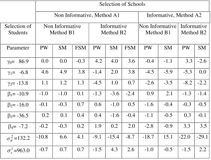
The results of the robustness study are exhibited in tables 4 and 5, which are analogous to Tables 2 and 3. Notice that the noninformative sampling schemes (Methods A1 and B1) were assumed to be known, so that the models assumed for the sampling probabilities in these cases are correct. The present robustness study is restricted therefore to situations where an informative sampling scheme at either level is misspecified.
Insert Tables 4 and 5 about here
The conclusions emerging from this study can be summarized as follows: Misspecification of the models assumed for the sampling probabilities has no biasing effect
on the estimation of the coefficients E E1... 4 and the variance 2
6
parameters under the assumption of ignorable sampling schemes also perform very well, and the percent relative biases of the corresponding point estimators (not shown) are in all the cases less than 3.2%. This outcome is very different from the results obtained under the selection schemes underlying the results in Table 1, where large biases were obtained when ignoring sample selection within the schools.
The results of the robustness simulation study are generally satisfactory also with respect to the estimation of the second level model coefficients. Except for the case of informative sampling of schools (Method A2) and informative sampling of pupils (Method B2) where the estimator of J2 has bias of about 8% under probability weighting, the biases of the estimators
of J0 and J2 are in all the other cases less than 4.5%. The biases of the estimators of J1 are
somewhat larger, but not much larger than the biases obtained under noninformative sampling of schools and pupils (Methods A1 and B1). The confidence intervals computed under the two approaches perform similarly in the case of J0, with undercoverage of up to 11
percentage points compared to the 95% nominal level, but ignoring the sample selection schemes in this case results in more severe undercoverage. The use of probability weighting yields confidence intervals for J1 andJ2 with undercoverage of up to 7 percentage points,
but the use of the sample models credibility intervals yields undercoverage of at most 2.5 percentage points under all four sampling schemes.
The two approaches are not robust with regard to the estimation of 2
u
V under the model misspecifications considered in the present study. Although the estimation of this variance is already problematic under correct model specification and even under noninformative sampling schemes (see the discussion in the comment at the end of Section 6), the biases under the misspecified models are even larger, particularly under informative selection of the schools when using the sample model, and under informative sampling of pupils (but noninformative sampling of schools), when applying the probability weighting approach. The percent undercoverage of the confidence intervals for 2
u
the credibility intervals for 2
u
V computed by use of the sample models perform generally better than the probability weighted confidence intervals, but an undercoverage of 14 percentage points is observed for the case where both sampling schemes are informative.
In summary, both probability weighting and the use of the sample model seem to be equally robust with regard to point estimation of the model coefficients, but the use of the sample models yields confidence (credibility) intervals with somewhat better coverage properties even under the misspecified models for the sample selection probabilities. The two
approaches fail to yield reliable point estimators and confidence intervals for 2
u
V , but as mentioned before, the estimation of this variance is known to be problematic even under the classical (population) multi-level model with no sampling effects.
8. FURTHER REMARKS AND CONCLUSIONS
An important message reinforced in the present study is that ignoring an informative sample selection scheme and fitting the population model may yield large biases of point estimators that distort the analysis. We describe and compare two approaches to control the bias. The first approach uses probability weighting to obtain approximately unbiased and consistent estimators for the corresponding census estimators under the randomization (repeated sampling) distribution. The census estimators are the hypothetical estimators computed from all the population values, and with large populations they can be expected to be sufficiently close to the true model parameters. The second approach attempts to identify the parametric model holding for the sample data as a function of the population model and the first order sample selection probabilities, and then fits the sample model to the sample data. The two approaches have been shown in the simulation experiment to remove the bias
of all the point estimators except in the case of the ‘between school’ variance 2
u
V , where with a small number of schools the use of probability weighting produces large biases under all the sampling schemes considered, including the non-informative scheme where both the selection of schools and the sampling of pupils within the selected schools is by simple random sampling. The use of the sample model likewise produces biased estimators for this variance with a small number of schools, and as discussed in Section 6, the bias depends also in this case on the choice of the corresponding prior distribution.
the population model, although the validation of the model under this approach is an open problem. The second advantage of this approach is that it is very simple and requires minimal computation resources, including the estimation of the variances of the point estimators. The use of this approach has, however, some serious limitations already discussed in the introduction. In particular, it requires large sample normality assumptions for the computation of confidence intervals.
The use of the sample model is more flexible and with the specification of appropriate prior distributions, it allows simulating from the posterior distribution of the target parameters. This advantage of the use of the sample model is demonstrated in Tables 3 and 5 where we compare the percentage coverage of confidence intervals produced by the two approaches. Inference based on the sample model requires, however, the specification of the conditional expectations of the sample selection probabilities at the various levels of the model hierarchy, given the values of the corresponding dependent and independent variables. As illustrated in the present study, these expectations may depend on a large number of unknown parameters that need to be estimated along with the population parameters. Application of this approach with the aid of MCMC simulations is computation intensive and as discussed in Section 6, with a small number of second level units, the performance of the variance estimators is rather erratic and may depend on the specification of the prior distributions, even when restricting to ‘non-informative’ priors. Nonetheless, with ‘correct’ specification of the sample model the use of this approach overcomes the inference limitations of probability weighting noted in the introduction.
The robustness study carried out in this article suggests that even quite drastic
misspecification of the models assumed for the sample selection probabilities may only have a modest effect on the estimation of the model coefficients and the performance of the corresponding confidence intervals, but large biasing effects are observed when estimating the ‘between school’ variance 2
u
REFERENCES
Anderson, T. W. (1973). Asymptotically efficient estimation of covariance structures with linear structure. Annals of Statistics, 1, 135-141.
Browne, W. J., and Draper, D. (2001). A comparison of Bayesian and likelihood-based methods for fitting multilevel models (unpublished manuscript).
Gelman, A. (2004). Prior distributions for variance parameters in Hierarchical models (unpublished manuscript).
Goldstein, H. (1986) Multilevel mixed linear model analysis using iterative generalised least squares. Biometrika, 73, 43-56.
Kovacevic, M. S., and Rai, S. N. (2003). A pseudo maximum likelihood approach to multilevel modelling of survey data. Communications in Statistics, Theory and Methods, 32, 103-121.
Pfeffermann, D., Skinner, C. J., Holmes, D. J., Goldstein, H., and Rasbash, J. (1998a). Weighting for unequal selection probabilities in multilevel models. Journal of the Royal Statistical Society, Series B, 60, 23-40.
Pfeffermann, D., Krieger, A.M., and Rinott, Y. (1998b). Parametric distributions of complex survey data under informative probability sampling. Statistica Sinica, 8, 1087-1114.
Pfeffermann, D., and Sverchkov, M. (1999). Parametric and semi-parametric estimation of regression models fitted to survey data. Sankhya, Series B, 61, 166-186.
Sampford, M. R. (1967). On sampling without replacement with unequal probabilities of selection. Biometrika, 54, 499-513.
Table 1.Percent relative bias (PRB) and p-values (P-V) of tests of bias when ignoring the sampling process.
Selection of Schools
Non Informative, Method A1 Informative, Method A2
Selection of
Students Non Informative Method B1 Informative Method B2 Non Informative Method B1 Informative Method B2
Parameter PRB P-V PRB P-V PRB P-V PRB P-V
J0= 86.9 0.5 3.1 9.2 0.0 -7.0 0.0 4.1 0.0
J1= -6.8 -4.1 22.2 27.3 0.0 0.9 79.0 27.1 0.0
J2= -13.8 -3.4 4.1 36.5 0.0 -0.7 67.6 37.2 0.0
E1= -10.9 -1.6 15.2 -13.7 0.0 0.7 52.8 -12.5 0.0
E2= -16.0 0.2 76.3 -13.9 0.0 0.9 27.3 -12.2 0.0
E3= -36.5 0.3 51.2 -16.1 0.0 0.3 57.0 -15.9 0.0
E4= -7.2 -1.0 57.8 -15.8 0.0 -0.1 93.8 -14.4 0.0
Vu2=132.2 6.8 0.0 -80.9 0.0 6.6 0.0 -79.9 0.0
Table 2. Percent relative bias (PRB) when accounting for the sampling process by use of probability weighting (PW), the sample model (SM), and the full sample model (FSM).
Selection of Schools
Non Informative, Method A1 Informative, Method A2
Selection of
Students Method B1 Non Informative Informative Method B2 Non Informative Method B1 Informative Method B2
Parameter PW SM FSM PW SM FSM PW SM PW SM
J0= 86.9 0.5 0.5 0.2 1.0 1.2 0.6 -1.2 -0.3 -0.3 0.2 J1= -6.8 -4.1 -4.1 -4.2 -0.4 -1.0 -1.4 4.7 -0.3 1.9 -3.0 J2= -13.8 -3.5 -3.4 -3.1 -1.3 -1.7 -2.7 -0.5 -1.5 -0.9 -1.4 E1= -10.9 -1.5 -1.6 -0.3 -2.3 -2.1 -0.3 2.3 1.9 -1.1 0.2 E2= -16.0 0.4 0.2 1.1 -2.5 -2.3 -0.9 1.4 1.6 -0.6 0.6 E3=-36.5 0.4 0.3 0.6 -2.7 -2.3 -0.7 0.7 0.5 -2.0 0.0 E4= -7.2 -0.8 -1.0 0.4 -3.4 -3.3 -1.3 -0.5 1.4 -4.3 -0.2
2
u
V =132.2 -10.6 6.8 4.3 -20.0 -14.7 -8.1 -15.1 4.8 -21.5 -6.5
2
8
[image:25.612.91.524.126.456.2]Table 3. Percent coverage of nominal 95% confidence intervals when ignoring the sampling process (IG), under probability weighting (PW), the sample model (SM) and the full sample model (FSM).
Selection of Schools
Non Informative, Method A1 Informative, Method A2
Selection of
Students Non Informative Method B1 Informative Method B2 Non Informative Method B1 Informative Method B2
Parameter PW SM =IG
FSM =IG
IG PW SM FSM IG PW SM IG PW SM
J0= 86.9 92.8 93.8 92.6 41.4 91.6 93.0 89.4 71.2 89.4 92.8 83.2 92.0 89.8 J1= -6.8 95.2 96.2 95.0 91.2 94.4 95.2 91.2 94.6 91.2 94.6 93.0 90.0 92.0 J2= -13.8 94.0 94.8 93.6 74.0 94.2 95.2 94.2 94.2 90.8 93.6 72.8 91.0 91.2 E1= -10.9 95.2 95.2 94.6 89.8 92.8 92.2 90.8 93.8 92.2 93.6 92.6 94.0 94.2 E2= -16.0 95.4 96.2 95.6 91.0 95.4 96.0 93.6 95.8 92.0 95.4 91.6 95.8 94.6 E3= -36.5 93.4 94.4 94.2 73.8 96.0 93.6 93.6 95.4 95.2 95.2 76.8 92.6 94.4 E4= -7.2 93.6 95.0 95.4 95.8 96.6 95.6 95.4 95.2 91.4 96.0 91.2 92.0 92.0
2
u
V =132.2 87.8 94.8 95.0 8.6 79.2 92.4 94.2 94.8 78.6 94.8 9.4 72.0 92.2
2
9
Table 4. Percent relative bias (PRB) when accounting for the sampling process by use of probability weighting (PW), the sample model (SM), and the full sample model (FSM); Robustness study.
Selection of Schools
Non Informative, Method A1 Informative, Method A2
Selection of
Students Non Informative Method B1 Informative Method B2 Non Informative Method B1 Informative Method B2
Parameter PW SM FSM PW SM FSM PW SM PW SM
J0= 86.9 0.0 0.0 -0.3 4.2 4.0 3.6 -0.4 -1.1 3.3 -2.6 J1= -6.8 4.6 4.9 3.8 -1.4 2.0 3.8 -4.5 -5.9 -5.3 0.0 J2= -13.8 1.1 1.2 1.3 -4.5 1.0 0.7 -2.6 -3.5 -8.2 -2.2 E1= -10.9 -1.0 -1.0 0.1 -1.3 -3.6 -2.4 0.9 2.1 -1.3 -1.4 E2= -16.0 -0.1 -0.3 0.7 0.6 -1.0 0.5 -1.6 -0.4 -0.3 -0.5 E3= -36.5 0.2 0.1 0.4 0.4 -1.6 -0.4 -1.1 -0.5 0.3 -0.1 E4= -7.2 -0.2 -0.3 0.2 1.9 0.2 2.0 -2.8 -0.9 3.3 3.5
2
u
V =132.2 -10.8 6.6 4.1 -9.1 -15.4 -8.7 -18.7 15.1 -22.0 -29.1
2
8
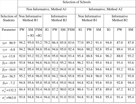
[image:27.612.94.521.114.438.2]Table 5. Percent coverage of nominal 95% confidence intervals when ignoring the sampling process (IG), under probability weighting (PW), the sample model (SM) and the full sample model (FSM); Robustness study.
Selection of Schools
Non Informative, Method A1 Informative, Method A2
Selection of
Students Non Informative Method B1 Informative Method B2 Non Informative Method B1 Informative Method B2
Parameter PW SM = IG
FSM =IG
IG PW SM FSM IG PW SM IG PW SM
J0= 86.9 94.2 95.0 93.2 79.2 86.4 85.8 83.6 77.0 89.2 91.4 94.8 87.0 87.8 J1= -6.8 94.2 96.0 94.8 95.6 94.6 95.0 92.4 94.6 90.2 92.8 95.4 89.4 93.4 J2= -13.8 92.0 93.2 92.2 95.6 95.0 94.8 93.4 95.4 88.8 94.4 96.2 88.0 93.2 E1= -10.9 93.8 94.6 94.8 94.6 93.4 95.2 94.4 96.2 93.4 95.4 94.4 93.4 93.6 E2= -16.0 94.2 95.4 95.8 93.8 92.2 94.0 91.0 94.2 93.6 94.6 94.8 93.2 93.6 E3= -36.5 95.2 95.6 96.0 95.8 94.2 94.8 95.8 95.8 94.8 96.0 93.8 91.2 93.0 E4= -7.2 94.8 95.6 95.8 95.8 95.4 95.0 94.8 94.8 92.8 93.6 95.0 92.8 94.4
2
u
V =132.2 84.4 93.8 93.4 94.8 87.2 90.0 92.8 90.4 71.4 87.8 89.0 67.2 81.2
2
8
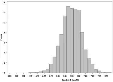
Figure 1. Histogram of actual sample of school sizes when the population school sizes are generated from the truncated t-distribution. Sampling scheme A2
[image:29.612.119.495.434.707.2]