Threshold Models with Correlated Random Components

Threshold Models with Correlated Random Components

Ayoub Saei

Abstract

Threshold models for ordinal longitudinal/repeated measurements data need to account for the

correlation between observations within each subject. Two variance-covariance structures are

introduced for two types of threshold models. Estimation of the parameters in the linear

predictor and components of variance are derived in the general form. A small simulation

study is carried out to support the estimation and inference methods. These methods are then

applied to two practical examples.

Threshold Models with Correlated Random Components

Ayoub Saei

Southampton Statistical Sciences Research Institute, University of Southampton, Highfield, Southampton SO17 1BJ, UK

Summary. Threshold models for ordinal longitudinal/repeated measurements data need to account for the correlation between observations within each subject. Two variance-covariance structures are introduced for two types of threshold models. Estimation of the parameters in the linear predictor and components of variance are derived in the general form. A small simulation study is carried out to support the estimation and inference methods. These methods are then applied to two practical examples.

1

.

Introduction

Ordinal or ordered categorical data often occur as response variables in statistical applications, although some arise from grouping an underlying continuous random variable. McCullagh and Nelder (1989) have summarised different situations, which result in such polytomous data. A particular polytomous data are ordinal response variables. A flexible and widely used model in analysing ordinal responses is the threshold model (ordinal regression model McCullagh 1980).

In many applications, the dependence structure is more complex than the independent observations assumed by the ordinal regression model of McCullagh (1980). In particular, observations often exhibit a clustering, and observations within clusters are correlated. A common instance of this occurs with longitudinal and repeated measurements where a cluster consists of the set of observations for a given subject. In this paper, we develop two types of models for the ordinal response variables, time dependent and time independent threshold models with correlated random effects.

equations (GEE) in Kenward, et al (1994) and Miller et al (1993) by GEE and weighted least squares.

Longitudinal and repeated measures models need to account for the correlation between observations within subjects. The models also need to show possible changes of the threshold parameters (cut-points) over time/space. This paper introduces two random components threshold models in analogue to Saei and McGilchrist (1998). The models allow the observations within a subject to be correlated. Sections 2 and 3 give models and estimation procedures. In sections 4 and 5 estimation equations are simplified for two particular types of variance-covariance matrices. Section 6 presents a small simulation study. Sections 7 and 8 apply the estimation methods to the unpublished microbial plaque data and respiratory disorder data of Koch et al (1990). The results of the paper are discussed in the last section.

2. Models

Suppose that repeated observations of an ordinal response variable Y are obtained (Y_it) at times t = 1,2,...,n from subject i, i=1, 2,...,N; Y_it can take on values 1, 2, ..., M.

The distribution of Yit depends on the linear predictor ηit xitc uit, where xit is a

vector of p known regression variables with fixed regression coefficient and u_it is a random variable. The random variables uit and uis for a subject are correlated; those from distinct subjects are independent. The random vector u_i [u_i1,u_i2,...u_ini]c is assumed

to follow multivariate normal distribution with variance-covariance matrix that is character-rised by variance and correlation parameters ϕ and ρ. The observable variable Y_it is the

categorised value of an unobservable continuous variable Vit with conditional mean of

it

the corresponding parameter at time t. Two cumulative distribution functions for Y_it conditional on uit, are then

) G(

)

P(Yit ≤k = θk −ηit (2.1)

) G(

)

P(Y_it ≤k = θ_kt −η_it (2.2) where k = 1, 2,..., M and G(.) is cumulative distribution function for an unobservable continuous random variable Vit with conditional mean ηit. Different choices of the

distribution function G(.) result in different threshold models. Four commonly consi-dered threshold models correspond to the four common distributions; standard normal, logistic, extreme minimal and extreme maximal for G(.). The results of threshold model with logistic distribution for G(.) are reported in this paper. Models (2.1) and (2.2) are called time independent and time dependent random component

threshold models respectively.

The parameter θ0 is always taken as -∝, so that G(θ0 - ηit) = 0 while θM is taken to be

+∞

identifia-bility since any quantity added to all values can be compensated by adding it also to the constant terms . This lack of identifiability is resolved by setting θ1 = 0. Thus

there are M - 2 and n(M - 2) unknown threshold parameters (θs) under models (2.1), (2.2) respectively, where n is the minimum of the nis. The threshold parameters are collected into a vector . In general can be expressed as =X Zu, where X is a known matrix of regression variables, Z is the incidence matrix for the random effect vector u and u=[u′1 ,u′2 ,...,u′N]′ ∼N(0, ϕA) with A=diag(Ai). The Ai are ni×ni

3. Estimation

In linear mixed models, best linear unbiased predictors (BLUP), Henderson (1963 1973,1975) are used to obtain maximum likelihood (ML) and restricted or residual maximum likelihood (REML) in Harville (1977), Thompson (1980), Fellner (1986, 1987) and Speed (1991). McGilchrist (1994) extends this approach to generalized linear mixed models for a broader class of problems. The method has elements in common with Schall (1991), Breslow and Clayton ( 1993), Wolfinger (1993), Nelder and Lee (1996) and Saei and McGilchrist (1998). Lee and Nelder (2001a, 2001b) further extend work of Nelder and Lee (1996) to the correlated non-normal data. An outline of the extension of Saei and McGilchrist (1998) to the correlated ordinal data is given here. Let l1 be

the loglikelihood function of ordinal observations conditional on the random component vector u taken to be fixed and l2 the logarithm of the probability density

function of u. The functions l1 and l2 are

] |

| ln ln const. )[ 2 / 1 (

ln

1 0

1 1

u A u

A 1

c

¦ ¦

ϕ ϕ

∆

N l

l

2 N i

n t it 1

i

where _is G( _{y is}) G( _{y 1 is})

is

is η θ η

θ

∆ and G( ) G( )

1) is s(y

is sy

is θ _is η θ _is η

∆

undser models (2.1) and (2.2) and N0 =

∑

estimators and their approximate variance-covariance matrices. Step 1. Estimates

_T

E

u

These estimates are then used as an initial step in finding ML and REML estimates of ϕ and ρ via Anderson (1973) and Henderson (1973) algorithm. Starting from initial

values k = 0, ₀, ₀, u0, ϕ0 and ρ0 (hence A0), the estimating equations set out by

» » » ¼ º « « « ¬ ª » ¼ º « ¬ ª » » » ¼ º « « « ¬ ª cc » » » ¼ º « « « ¬ ª » » » ¼ º « « « ¬ ª k k k k k k k k k u A V Z X I V u u 1 0 1 1 1 1 1 1 1 0 0 / l / l 0 0 0 ∂ ∂ ∂ ∂ (3.1) where » » » ¼ º « « « ¬ ª »¼ º «¬ ª ¸¸¹ · ¨¨© § » ¼ º « ¬ ª c c c c » » » ¼ º « « « ¬ ª

cc 1

0 1 0 1 2 1 2 1 2 1 2 0 0 0 0 0 0 0 0 / / / / A Z X 0 0 0 I Z 0 X 0 0 I V ϕ ∂ ∂ ∂ ∂ ∂ ∂ ∂ ∂ ∂ ∂ ∂ ∂ k k k k k k k k l l l l , k k k k k k k

k l l l l

l ∂ ∂ ∂ ∂ ∂ ∂ ′ ∂ ∂ ∂ ′ ∂ ∂ ∂ ′

∂ / , / , / , / and 2₁/

1 2 1

2 1

1 are evaluated at

initial estimates of the parameters.

Step 2. Once iterations of (3.1) have converged to ~ and u~ , let ~ X~Zu~,

B _∂2_l1/_∂~_∂~c_, 1 T 1

0 1 0 * _{[ ]} Z BZ A

T ϕ . The ML estimate of the variance

component parameter ϕ is estimated by

ˆ ( ) [tr( ( ) *) ~ ( ₀)~]

0 -1 1

1 A T uA u

-1 _ρ

ρ

ϕ c

¦

i ni (3.2)

The evaluation of (3.1) and (3.2) is then iterated with initial values set to ~, ~, u~

and ϕˆ. Step 3. After convergence of steps 1 and 2, the ML estimate of the correlation

parameter ρ is

ρˆ h(.) (3.3 )

where h(.) is a function of tr{(_∂A−1/_∂ρ0)_A(_ρ0)}_{, ˆ [tr{( / )} *_}] 0 1 1

(ML) A ∂ρ T

ϕ− _∂ − _and

u A

u~_′(_∂ −1/_∂ρ0)~_{. Note that evaluation of the h(.) components depends on}

varinac-covariance matrix of the random effect u. The new values ~, ~, u~ , ϕˆ and ρˆ are

substituted for 0, 0, u0, ϕ0 and ρ0 in (3.1), and then (3.1) - (3.3) are evaluated again.

At convergence, ϕˆ and ρˆ are ML estimates (ϕˆ_(ML) and ρˆ_(ML)) of ϕ and ρ with

Var( _» ¼ º « ¬ ª (ML) (ML) ˆ ˆ ρ ϕ

) = 2 1

(11) 1 11 (11) 11 2 11 1 1 1 1 11 4 1 0 2 ) 2 ( . ) -2 ( ) 2 (N » ¼ º « ¬ ª k k k k r r ν ϕ ϕ ν ϕ ϕ

ϕ _(3.4)

where N0 =

∑

Let           = 33 32 31 23 22 21 13 12 11 V V V V V V V V V V and           = − 33 23 22 13 12 11 1 . . . T T T T T T

V be the partitions of the matrix

V and its inverse corresponding to the dimensions of the , and u. Replacing _T*

by T33 in all above three steps (3.1 - .3.3) yields REML estimates of the parameters

and variance components ϕ and ρ. Similarly, replacing _T* _{by T}

33 in (3.4) gives the

asymptotic variance-covariance matrix for the REML estimators ϕˆ(REML) and ρˆ(REML).

4. Exchangeable and AR(1) Models

A simple form of dependence arises when the random components of u have an exchangeable correlation (constant correlation) ρ. The variance covariance matrix for

the random components u is ρA where A is a block diagonal matrix with blocks Ai =

i i J I ρ ρ + − ) 1

( and i = 1,2,..., N; Ii is an ni×ni identity matrix and Ji is a ni×ni

matrix with all elements equal to 1. Let *

[ ]

ij

T

T = with *

ij

T as a n_iun_j matrix, the ML

estimation equation for ρ, i.e., h(.) in (3.3) is then ρˆ=-(a b c)-1d

0 2

0 ρ

ρ ,

where

¦

¦

N

i i i i i i i i i i

N

i ni ni 1 n 1 2 n 3 4 n n n

2 -1 1 2 )] 1)(2 ( )) b 1)(b ( ) b (b 1) (( [ b , 1) ( a ϕ ). ( tr = b and ~ ~ b , ) ( tr b , ~ ~ b , )] b (b ) b [(b d ], 1) ( ) b (b [ 2 c * 4 3 * 2 1

=1 1 2 3 4

-1

1 1 2

-1 ii i i i i i i ii i i i i N

i i i i i

N

i i i ni ni u

T J u J u T u c c

¦

¦

matrix of the random components u is ϕA, where A is a block diagonal matrix with

the blocks _{Ai =}

(

)

[ ]

st = ρ|s-t| , and s, t = 1, 2,…, ni. Let a = 2(1−ρ−2)−1N ,

i N i i i N

i ii i

u u

T ) ~ ~

( tr

b ₁

1

*

∑

∑

=

′ +

= and N N_{i i i i}

i ii i

u u

T ) ~ ~

( tr

c ₁

1

*

∑

∑

=

′ +

= , the h(.) in (3.3) is

ρˆ=-(a₊2_ϕˆ-1b)-1_ϕˆ-1c

where _i is a n_i×n_i diagonal matrix with diagonal elements (0,1,…,1,0) and _i is a

i i n

n × matrix and has -1 above and below principal diagonal and zero all other

elements. The REML counterparts are obtained by replacing _T* _{by T} 33.

5. Simulation

A limited simulation study was undertaken to examine the performance of the method for several parameter combinations. Observations were generated from time independent threshold model P(Yit ≤y)=G(θy−ηit) where G(.) is the logistic function and

it it it =β0+x β1+u

η . The uit are generated from an AR(1) with parametees ρ and ϕ.

The xit are randomly assigned to 1 or 0 and observations are obtained at time t = 1, 2,…, 5 for i = 1, 2,…, 30. Estimates of parameters are obtained, and the process is replicated 1000 times. Table 1 shows the results by REML method for the different combinations of the parameters in the variances in which ρ and ϕ are allowed to change. The threshold and fixed parameters are held constant. The quantities are reported in Table 1 are the true parameters values (TV), the average of the biases (AB), standard error over 1000 simulations (SE1) and the average asymptotic standard error of 1000 simulations (SE2).

REML method reduces biases of the estimators. With increased variance components the bias of the estimator ϕ is increased. The relative bias (bias/(true value)) of

estimating ρ is much smaller than for ϕ. The bias of the REML estimator of ρ is not

significant for the parameter set 3. The biases of the estimators of β0 and β1 are small

and their standard errors over simulation SE1 are in agreement with SE2 in both ML and REML methods. This is also true for the correlation parameter ρ. However, the

SE2 of the estimator of ϕ is greater than SE1. This indicates that the method

overestimates the standard error of the estimator of ϕ. However, the results of other simulations (not reported) show that the difference between SE1 and SE2 decreases by increasing the number of subjects from 30 to 100.

6. Application To Microbial Plaque Data

The preceding theory is applied to unpublished microbial plaque data. The data are obtained from Nasr Isfahani. A study was planned to determine the effective time of brushing teeth according to Bass method by Nasr Isfahani (1999). A total of 60 dentist students were randomly selected and assigned to 6 groups of 10 each students. The students were asked not to use any procedure to remove plaque 24 hours before the visit. At the baseline and after brushing teeth for 1, 2,… , 6 minutes, the plaque indices (sinless and loe plaque index) were recorded on a four point ordinal scale (0 = excellent, 1 = good, 2 = not bad and 3 = bad) for all four tooth surfaces (mesial, distal, fasial and lingual). Data on tooth number 1 in the upper-left quadrant are used here. The model fitted is

ηis β0βt(timei)ωj(basei)uis

at base-line and uis is the sth tooth surface (s =1= mesial, s = 2 =distal, s = 3 = fasial

and s = 4 = lingual) random effect for student i. Random vector ui =

(

)

is a multivariate normal with zero mean and exchangeable variance-covariance structure. Note that the AR(1) model is not fitted since the distance between two-tooth surfaces can not be meaningfully defined.

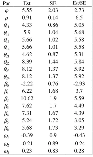
Table 2 shows the results for the time dependent threshold model (2.2). There is a significant variation between students with REML estimate value of ϕ = 5.55 and standard error of 2.03. The random effects for a student are highly correlated.

The paired comparisons show that there is a statistically significant changes from β1 to β2 but not from β2, β3, … , β6. This indicates that the effective time to remove

plaque is between 2 and 3 minutes. The initial value of plaque has no statistically significant effect.

The results also shows that the threshold parameters θks (k =1,2 and s = 1, 2, … , 4) have statistically significant changes over four tooth surfaces (mesial, distal, fasial and lingual). The model (2.2) yields the same predicted values as observed in 88.3%.

7. Application to Respiratory Disorder Data

A second application is to respiratory disorder given by Koch et al (1990). A total of 111 patients within two centres were randomly assigned to two treatments (active, placebo). At the baseline, status of each patient was recorded according to a five point ordinal response scale (0 = terrible, 1 = poor, 2 = fair, 3 = good, 4 = excellent), and also at each of four visits (visit 1, visit 2, visit 3, visit 4) during the time period over which the treatments were administrated. Patients’ characteristics like age and gender were also recorded at the time of entry to the study. The model is

where risk variables are centre (ci, 1 = centre 1, 0 = centre 2), age in years at base-line (agei), gender (geni, 1 = male, 2 = famle ), status at base-line (stuti, j = 1, 2,… , 5), treatment (treatit, 1 = active, 0 = placebo) and uit is ith patient random effect. The results of fitting model (8.1) via REML method for AR(1) are given in Table 3.

The results show that the random components are highly correlated for a patient with REML estimate of ρ = 0.9 and standard error of 0.04. The center, gender effects α, λ

and age regression coefficient γ are not significant. The initial status of patients has a statistically significant effect. It indicates that patients with status in lower category (terrible) at base-line tend to give response in lower category in the end of study. Although the treatment effect βt increases from the first visit to the second and then decreases, the paired comparisons show that the changes are not statistically significant.

By using asymptotic distribution of the estimators βt and assuming that the βt are constant over time, it can be seen that the treatment is highly statistically significant. The estimate of treatment effect is positive, indicating that patients in the treatment active group are more likely to respond in the higher categories. The results (not reported in the paper) of fitting model (2.2) show that the changes of the threshold parameters over time are not statistically significant. Under model (2.1), the observed and predicted values agree in 66.8% and 72.8% for an exchangeable and an AR(1) models respectively. These percentages show that the model (2.1) with AR(1) correlation structure is a suitable model for this data.

8. Discussion

takes into account possible changes of the threshold parameters over time. The estimation and inference approaches have been applied to two data sets. The results (Tables 2 and 3) show that observations are highly correlated within clusters in both applications. The threshold parameters have significant changes over four tooth surfaces in the first application. These parameters are constant over time period of study in the second application. Although the threshold parameters are changing over four tooth surfaces, the conclusions do not change from the model (2.1) to the model (2.2). However, in another application (submitted for the publication) the significant changes of the threshold parameters yielded different conclusions from the models (2.1) and (2.2). The results of a limited simulation (Table 1) show that the REML estimates of the fixed effect and threshold parameters are very good. The REML estimates are even unbiased for some of those parameters. The REML estimator of the variance parameter ϕ is negatively biased. However, the bias of the REML estimator for the

correlation parameter ρ is very small. The method provides very good estimates of the

standard error of and correlation parameter ρ. It overestimates the standard error of

the estimator of ϕ.

The goodness of fit of the model is based on a simple method of Saei and McGilchrist (1998). Further work is needed on the goodness of fit of the model. The biases in estimation of the variance component ϕ and its standard error are the other problems of the method.

Appendix A

The elements in the asymptotic variance-covaraince matrix (3.4) for the ML

] ) / ( tr[ 1

1 A ρ A

ν = ∂ − ∂ _{, tr[(} 1_{/ )} 1₍ 1_{/ )} 1_] 11= ∂A− ∂ρ A− ∂A− ∂ρ A−

ν ,

k11= tr[T*(∂A−1/∂ρ)T*A−1], k11(11)=tr[T*(∂A−1/∂ρ)T*(∂A−1/∂ρ)]

and

] ) / ( ) / (

tr[ 1 * 1

1 (11)

1 =ϕ− ∂A− ∂ρ T ∂A− ∂ρ A

k .

The replacement of _T* _{by T}

33 yields corresponding components for the asymptotic

variance-covariance matrix of the REML estimtors of

ϕ

and

ρ

.

References

Anderson, T.W. (1973) Asymptotically efficient estimation of covariance matrices with linear structure. Annals of Statistics1, 135-141.

Breslow, N.E. and Clayton, D.G. (1993) Approximate inference in generalised linear mixed models. Journal of the American Statistical Association 88, 9-25.

Crouchley, R. (1995) A random effects model for ordered categorical data. Journal of

the American Statistical Association 90, 489-498.

Hedeker, D. and Gibbons, R.D. (1994). A random effects ordinal regression model for multilevel analysis. Biometrics50, 933-944.

Henderson, C.R. (1963) Selection index and expected genetic advance. In Statistical

Genetics and Plant Breeding (W.D. Hanson and H.F. Robinson, eds.), 141-163.

National Academy of Sciences and National Research Council Publication No. 982, Washington, D.C.

Henderson, C.R. (1973) Sire evaluation and genetic trends. In proceedings of the

Animal Breeding and Genetics Symposium in Honour of Dr. Jay L. Lush 10-41.

Amer. Soc. Animal Sci.-Amer. Dairy Sci. Assn.-Poultry Sci. Assn. Champaign, III. Henderson, C.R. (1973) Maximum likelihood estimation of variance components,

Henderson, C.R. (1975) Best linear unbiased estimation and prediction under selection model. Biometrics31, 423-447.

Hougaard, P. (1986) Survival models for heterogeneous populations derived from stable distributions. Biometrics 73, 387-396.

Jansen, J. (1990) On the statistical analysis of ordinal data when extra variation is present. Applied Statistics 39, 75-84.

Jansen, J. (1992) Statistical analysis of ordinal data from experiments with nested errors. Computational Statistics & Data Analysis 13, 319-330.

Kenward, M.G., Lesaffre, E. and Molenberghs, G. (1994) An application of maximum likelihood and generalized estimating equations to the analysis of ordinal data from a longitudinal study with cases missing at random. Biometrics50, 945-953.

Koch,G.G., et al (1990) Categorical data analysis. Statistical Methodology in the

Pharmaceutical Sciences. Eds. Donald A. Berry

McCullagh, P. (1980) Regression models for ordinal data. Journal of the Royal

Statistical Society B, 42, 109-142.

McCullagh, P. and Nelder, J.A. (1989) Generalized linear models. Second Ed. London:Chapman and Hall.

McGilchrist, C.A. (1994) Estimation in generalized mixed models. Journal of the

Royal Statistical Society Series B 56, 61-69.

Miller, M.E., Davis, C.S. and Landis, J.R. (1993) The analysis of longitudinal polytomous data: generalized estimation equations and connections with weighted least squares. Biometrics49, 1033-1044.

Nelder, J.A. and Lee, Y. (1996) Hierarchical generalized linear models. Journal of the

Lee, Y. and Nelder, J.A. (2001a) Hierarchical generalized linear models: A synthesis of generalised linear models, random-effect model and structured dispersions.

Biometrika88, 987-1006.

Lee, Y. and Nelder, J.A. (2001b) Modelling and analysing correlated non-normal data. Statistical Modelling1, 3-16

Nasr Isfahani, M. (1999) Effective time brushing to remove macrobial plaque by Bass method. MD thesis.

Saei, A. and McGilchrist, C.A. (1996) Random component threshold models. Journal

of Agricultural, Biological and Environmental Statistics 1, 288-296

Saei, A. and McGilchrist, C.A. (1997) Random threshold models for inflated zero class data. Australian Journal of Statistics39, 5-16.

Saei, A., Ward, J. and McGilchrist, C.A. (1996) Threshold models in methadone program evaluation. Statistics in Medicine15, 2253-2260.

Saei, A. and McGilchrist, C. (1998) Longitudinal threshold models with random components. The Statistician, Series D 47, 365-375.

Schall, R (1991) Estimation in generalised linear models with random effects.

Biometrika 78, 719-727.

Speed, T. (1991) Comment on Robinson: Estimation of random effect. Statistical

Science 6, 42-44.

Ten Have T. (1996) A mixed effects model for multivariate ordinal response data including correlated discrete failure time with ordinal responses. Biometrics53, 473-491.

Wolfinger, R. (1993) Laplace’s approximation for nonlinear mixed models.

Zhaorong, J., McGilchrist, C.A. and Jorgensen, M.A. (1992) Mixed model discrete regression. Biometrical Journal 34, 691-700.

Table 1.

REML estimation for the simulated data.

ϕ ρ θ1 θ2 θ3 θ4 β0 β1

TV 0.5 0.1 0.5 2 3.5 5 0.5 1 Par 1 AB -0.06 -0.08 0.0 -0.03 -0.06 0.07 -0.01 0.06

SE1 0.11 0.44 0.11 0.21 0.31 0.56 0.25 0.24 SE2 0.46 0.58 0.12 0.22 0.34 0.66 0.26 0.25 TV 0.5 0.3 0.5 2 3.5 5 0.5 1 Par 2 AB -0.05 -0.11 0.1 -0.05 -0.06 0.03 -0.02 0.04

SE1 0.12 0.44 0.12 0.22 0.34 0.51 0.26 0.24 SE2 0.46 0.56 0.12 0.22 0.34 0.66 0.26 0.25 TV 1 0.7 0.5 2 3.5 5 0.5 1 Par 3 AB -0.45 0.01 -0.04 -0.21 -0.33 -0.31 -0.04 0.04

SE1 0.26 0.21 0.11 0.22 0.32 0.54 0.31 0.34 SE2 0.48 0.25 0.12 0.22 0.31 0.54 0.34 0.33

* Par i = Parameter set i (i = 1, 2, 3).

Table 2.REML estimates of parameter Table 3. REML estimates of parameter (Est), standard errors (SE),z-value (Est/SE). (Est), standard error (SE),z-value (Est/SE).

Par Est SE Est/SE Par Est SE Est/SE

ϕ 5.55 2.03 2.73 ϕ 0.75 0.37 2.01

ρ 0.91 0.14 6.5 ρ 0.9 0.04 22.5

θ11 4.33 0.86 5.05 θ1 1.55 0.23 6.78

θ12 5.9 1.04 5.68 θ2 4.05 0.3 13.74

θ13 5.66 1.02 5.58 θ3 5.97 0.33 17.94

θ14 5.66 1.01 5.58 β0 7.01 1.11 6.29

θ21 4.62 0.87 5.31 β1 1.65 0.53 3.1

θ22 8.39 1.44 5.84 β2 2.36 0.55 4.31

θ23 8.12 1.37 5.92 β3 2.08 0.54 3.82

θ24 8.12 1.37 5.92 β4 1.57 0.54 2.93

β0 -2.22 0.76 -2.93 α -0.62 0.49 -1.27

β1 6.22 1.68 3.7 γ -0.03 0.02 -1.52

β2 10.62 1.9 5.59 λ -0.56 0.61 -0.92

β3 7.62 1.7 4.49 ω1 -4.46 1.5 -2.97

β4 7.31 1.67 4.39 ω2 -3.78 0.83 -4.55

β5 5.24 1.72 3.05 ω3 -2.41 0.73 -3.32

β6 5.68 1.73 3.29 ω4 -0.66 0.74 -0.9

ω1 -0.39 0.9 -0.43 *ω5 is fixed at zero to achieve identifiability

ω2 -0.21 0.89 -0.24

ω3 0.23 0.83 0.28

•Par = Parameter