A SEARCH ALGORITHM FOR A CLASS OF OPTIMAL FINITE-PRECISION CONTROLLER REALIZATION PROBLEMS
WITH SADDLE POINTS∗
JUN WU†, SHENG CHEN‡, GANG LI§, AND JIAN CHU†
Abstract. With game theory, we review the optimal digital controller realization problems that maximize a finite word length (FWL) closed-loop stability measure. For a large class of these optimal FWL controller realization problems which have saddle points, a minimax-based search algorithm is derived for finding a global optimal solution. The algorithm consists of two stages. In the first stage, the closed form of a transformation set is constructed which contains global optimal solutions. In the second stage, a subgradient approach searches this transformation set to obtain a global optimal solution. This algorithm does not suffer from the usual drawbacks associated with using direct numerical optimization methods to tackle these FWL realization problems. Furthermore, for a small class of optimal FWL controller realization problems which have no saddle point, the proposed algorithm also provides useful information to help solve them.
Key words. closed-loop stability, digital controller, finite word length, game theory, optimiza-tion, saddle points
AMS subject classifications. 93D99, 91A80, 15A18, 90C47, 90C90, 90C30
DOI.10.1137/S0363012903435084
1. Introduction. There has been a growing awareness that finite-precision con-troller implementation can have a serious influence on the actual performance of a digital closed-loop control system [1], [2], [3]. Due to the finite word length (FWL) errors, a casual controller implementation may degrade the designed closed-loop per-formance, or even destabilize the designed stable closed-loop system, if the controller implementation structure is not carefully chosen. The FWL effect has become more critical with the growing popularity of robust controller design methods which focus only on dealing with large plant uncertainty and result in controllers of much higher order and complexity than traditional classical control [2]. There are generally two types of FWL errors in the digital controller implementation. The first one is the rounding errors that occur in arithmetic operations [4], [5], and the second one is the controller parameter representation errors which have critical influence on closed-loop stability [6], [7], [8], [9], [10], [11], [12]. Typically, these two types of errors are investigated separately for the reason of mathematical tractability.
In general, there exist two different strategies, called the direct and indirect strate-gies, for constructing digital controllers that can tolerate FWL implementation errors. For the indirect strategy, the transfer function of the digital controller has been
de-∗Received by the editors September 25, 2003; accepted for publication (in revised form) May 17,
2005; published electronically November 23, 2005. http://www.siam.org/journals/sicon/44-5/43508.html
†National Key Laboratory of Industrial Control Technology, Institute of Advanced
Pro-cess Control, Zhejiang University, Hangzhou, 310027, People’s Republic of China. These au-thors were supported by the National Natural Science Foundation of China (grants 60174026, 60374002, and 60421002) and 973 program of China (grant 2002CB312200) ([email protected], [email protected]).
‡Corresponding author. School of Electronics and Computer Science, University of Southampton,
Highfield, Southampton SO17 1BJ, UK ([email protected]). This author was supported by the United Kingdom Royal Academy of Engineering.
§School of Electrical and Electronic Engineering, Nanyang Technological University, Singapore
signed by some controller synthesis methods. It is well known that a transfer function can be fulfilled with different realizations, and different realizations possess different degrees of robustness to FWL errors. This property can be utilized to select “opti-mal” realizations that optimize some FWL performance measures. Various FWL per-formance measures have been investigated, and these include the averaged roundoff noise gain [5], the complex stability radius measure [6], the transfer function sensitiv-ity measure [7], thel1-based stability measure [8], the Frobenius-norm pole sensitivity measure [9], and the 1-norm pole sensitivity measure [10], [11]. In the direct strat-egy, controller design involves explicitly the considerations of FWL implementation. By extending the standard H∞ control design to include FWL controller parameter perturbations, the work of [12] developed a Riccati inequality approach, which di-rectly obtains optimal controller realizations satisfying both theH∞ robustness and FWL closed-loop stability requirements. Similarly, by extending the standard linear quadratic Gaussian (LQG) control design to include the effects of FWL roundoff noise, the work of [4] developed a FWL-LQG controller design method. The direct strategy appears to be better than the indirect strategy, since the former does not make spe-cific assumptions on the controller, and in theory it should be a preferred approach. However, except for a few methods, such as H∞ and LQG, it is very difficult to ex-tend various controller design methods to this direct strategy. But this difficulty does not exist in the indirect strategy, where controller synthesis and controller realization are two separate steps. Various existing controller design methods can be used to attain a transfer function or an initial realization of the controller, which can then be optimized to satisfy FWL implementation requirements.
This paper adopts the indirect strategy with the Frobenius-norm pole sensitivity measure proposed in [9]. Our motivation is as follows. The Frobenius-norm pole sensitivity measure was derived in [9], and the optimal controller realization problem was defined as the maximization of this measure over all the possible controller re-alizations. An analytical solution to this class of optimal realization problems was attempted in [9]. However, it was pointed out that the conditions presented in [9] are not sufficient to provide an optimal realization [13]. Consequently, the solution expression presented in [9] is in general a suboptimal solution, and numerical op-timization methods have to be adopted [14] to find optimal solutions. Since these optimal FWL realization problems are highly complicated nonlinear and nonconvex optimization problems, especially when the order of the controller is large, a direct nu-merical optimization is computationally very expensive. Moreover, chances of search being trapped at some bad local solutions increase for large-scale problems, and it is impossible to tell whether or not a solution obtained is a global optimum. In this pa-per, these optimal FWL controller realization problems are reviewed with game theory [15], [16]. They are consequently divided into two types: optimization problems which have saddle points and optimization problems which do not have a saddle point.
remainder of the paper is organized as follows. Section 2 defines the optimal FWL controller realization problem considered in this study and introduces some necessary mathematical preliminaries. In section 3, the proposed two-stage search algorithm is derived. Section 4 discusses the practical value of this algorithm. Section 5 presents several design examples, and the paper concludes with section 6.
2. Problem definition and preliminaries. For a complex-valued matrixM= [mij],MT is the transposed matrix ofM,MH is the Hermitian adjoint matrix ofM, M∗ is conjugate toM,
Mmax= max i,j |mij|, (1)
and the Frobenius norm is defined as
MF =
i,j
|mij|2 1/2
.
(2)
Let Vec(·) be the column stacking operator such that Vec(M) is a vector. For a real-valued positive semidefinite matrixD≥0, the matrixD1/2 satisfiesD1/2(D1/2)T = D. For two real-valued matrices M = [mij] and N = [nij] of the same dimension, denote
M,N= i,j
mijnij. (3)
2.1. Problem definition. Consider the discrete-time closed-loop control sys-tem, consisting of a linear time-invariant plant P(z) and a digital controller C(z). The plant modelP(z) is assumed to be strictly proper with a state-space description
xP(t+ 1) =APxP(t) +BPu(t),
z(t) =CPxP(t),
(4)
where AP ∈ Rm×m, BP ∈ Rm×l, and CP ∈ Rq×m. The digital controller C(z) is described by
xC(t+ 1) =ACxC(t) +BCz(t), u(t) =CCxC(t) +DCz(t), (5)
withAC ∈ Rn×n,BC ∈ Rn×q,CC∈ Rl×n, andDC ∈ Rl×q. Denote therealization ofC(z) as
X=
DC CC
BC AC
.
(6)
Assume that an initial realization ofC(z),
X0=
D0C C0C B0C A0C
,
(7)
has been given by some controller synthesis method. Then all the realizations ofC(z) form a set
SC=
X:X=X(T) =
I 0
0 T−1
X0
I 0
0 T
,
where the transformationT∈ Rn×n is an arbitrary nonsingular matrix, and0andI denote the zero and identity matrices of appropriate dimensions, respectively. SC is not a convex set, as
λ
I 0
0 T−11
X0
I 0
0 T1
+ (1−λ)
I 0
0 T−21
X0
I 0
0 T2 (9)
may not belong to SC for any nonsingular T1,T2 ∈ Rn×n and 0 < λ < 1. The stability of the loop control system depends on the eigenvalues of the closed-loop transition matrix
A(X) =
AP +BPDCCP BPCC
BCCP AC
(10)
=
AP 0
0 0
+
BP 0
0 I
X
CP 0
0 I
=M0+M1XM2.
All the different realizationsXinSChave exactly the same set of closed-loop poles if they are implemented with infinite precision. Since the closed-loop system has been designed to be stable, all the eigenvalues λk(A(X)), 1 ≤ k ≤ m+n, of A(X) are within the unit disk.
WhenXis implemented with an FWL digital processor of fixed-point format, it is perturbed toX+ ΔX. Each element of ΔXis bounded by±ε; that is,ΔXmax≤
ε, where ε is the maximum representation error of the digital processor. With the perturbation ΔX,λk(A(X)) is moved toλk(A(X+ ΔX)). If an eigenvalue ofA(X+ ΔX) is outside the open unit disk, the closed-loop system, designed to be stable, becomes unstable with the finite-precision implementedX. It is therefore critical to know when the FWL error will cause closed-loop instability. This means that we would like to know the largest open “hypercube” in the perturbation space within which the closed-loop system remains stable. The size of this perturbation hypercube quantifies the FWL characteristics of X and is therefore a true FWL closed-loop stability measure forX[17].
Computing the size of this largest stable perturbation hypercube, however, is an unsolved open problem. An approximation to this true FWL closed-loop stability measure is the following Frobenius-norm pole sensitivity measure defined in [9]:
f(X)= min k∈{1,...,m+n}
1− |λk(A(X))| (l+n)(q+n)∂λk(A(X))
∂X F
.
(11)
Rigorous discussions regarding the rationality off(X) as an FWL closed-loop stability measure can be found in [9], [11]. Basically, under some mild assumptions and using a first-order approximation, it can be shown that the closed-loop system remains stable if ΔXmax < f(X). It has been argued in [18] that estimates obtained from first-order perturbation theory are often more realistic than rigorous bounds obtained by other means. Thus, the larger f(X) is, the larger an FWL error ΔX that the closed-loop system can tolerate. Moreover, f(X) is computationally tractable, as is summarized in the following lemma given by [19].
Lemma 1. Let A(X) = M0+M1XM2 given in (10) be diagonalizable.
reciprocal left eigenvector yk related to pk is obtained from [y1,y2, . . . ,ym+n] = [p1,p2, . . . ,pm+n]−H. Then
∂λk(A(X))
∂X =M
T 1y∗kp
T kM
T
2 ∀k∈ {1, . . . , m+n}. (12)
As different controller realizationsXresult in different values off(X), it is natural to search for “optimal” controller realizations that maximize the measure defined in (11). This leads to the following optimal FWL realization problem [9]:
υ= max X∈SC
f(X).
(13)
Numerical optimization methods have been used to attain solutions of this optimal realization problem (e.g., [14]). In general, the optimization problem (13) is highly nonlinear and nonconvex. Thus, numerical optimization methods do not guarantee attaining a global optimal solution and suffer from high costs, particularly for large-scale systems.
Now, let us define
g(X, k)= 1− |λk(A(X))| (l+n)(q+n)∂λk(A(X))
∂X F
.
(14)
Obviously, the optimal FWL realization problem (13) can be viewed as
υ= max X∈SC
min k∈{1,...,m+n}
g(X, k).
(15)
2.2. Saddle points and minimax theorem. This subsection introduces with-out proofs some properties of saddle points and the minimax theorem, which are useful in solving the optimization problem (15). The detailed discussion of this topic can be found in the standard game theory textbooks, such as [15], [16].
Definition 1. (X, k) ∈ SC× {1, . . . , m+n} is said to be a saddle point of g(X, k) if
g(X, k)≤g(X, k)≤g(X, k) ∀X∈ SC, ∀k∈ {1, . . . , m+n}. (16)
Theorem 1. If both (X, k)and(X, k)are saddle points of g(X, k), then
g(X, k) =g(X, k).
(17)
The following theorem is the well-known minimax theorem in game theory.
Theorem 2. If and only if there exists at least a saddle point(X, k)ofg(X, k),
then
max X∈SC
min k∈{1,...,m+n}
g(X, k) = min k∈{1,...,m+n}
max X∈SC
g(X, k) =g(X, k).
(18)
A direct corollary of Theorem 2 is stated as follows.
Corollary 1. If g(X, k)has no saddle point, then
max X∈SC
min k∈{1,...,m+n}
g(X, k)< min k∈{1,...,m+n}
max X∈SC
g(X, k).
g
(
X
,
k
)
X
g( X,1) g( X,2) g( X,3)
ρ1 ρ2 ρ3
q
1 q2 q3 q4
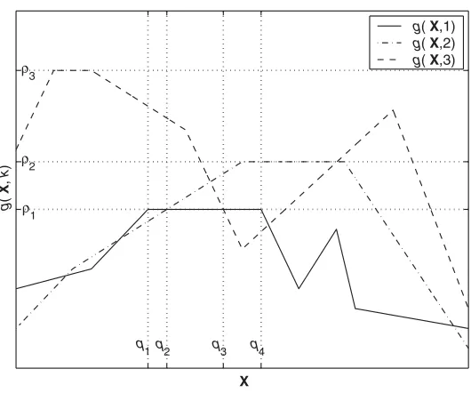
Fig. 1.A simple illustration ofρk,X, and saddle points.
Theorems 1 and 2 show that for the optimal FWL realization problem (15) which has saddle points, any saddle point of g(X, k) is a global optimal solution of (15). Define
ρk
= max X∈SC
g(X, k) (20)
fork∈ {1, . . . , m+n}and the index
k = arg min k∈{1,...,m+n}ρk. (21)
There exist an infinite number ofX∈ SC such thatg(X, k) =ρk. Define
X ={X:g(X, k) =ρk,X∈ SC}. (22)
Figure 1 depicts a simple illustration for a case of ρk withk ∈ {1,2,3}. It is easily seen that in this case X is the segment between q1 and q4 on the X-axis. It can also be observed in Figure 1 that the points between q2 andq3 (a subset ofX) are the realizations corresponding to saddle points. This observation accords with the following theorem, which provides a method for finding a saddle point.
Theorem 3. If and only if X∈ X satisfies
g(X, k)≥ρk ∀k∈ {1, . . . , m+n} \ {k},
(23)
then(X, k)is a saddle point of g(X, k).
[image:6.612.125.390.93.314.2]discussed in section 4. Based on Theorem 3, a two-stage algorithm is developed to find a saddle point of the optimal FWL controller realization problem (15). The first stage focuses the attention on solving the optimization problem (20) fork∈ {1, . . . , m+n}, and the indexk and the closed-form expression ofX are obtained in this stage. The second stage searches X for a controller realization Xopt that meets the condition
g(Xopt, k)≥ρk ∀k∈ {1, . . . , m+n} \ {k}. Such anXoptis a global optimal solution to the optimal FWL controller realization problem (13). We now discuss this two-stage algorithm in detail.
3.1. Stage 1 of the algorithm. It is known easily from (8) and (10) that
A(X) =
I 0
0 T−1
A(X0)
I 0
0 T
.
(24)
This means that ∀X ∈ SC, λk(A(X)) = λk(A(X0)). Thus, from (14), solving the maximization problem (20) is equivalent to solving the following minimization prob-lem:
ηk = min X∈SC
∂λk(A(X))
∂X F
.
(25)
Combining Lemma 1 with the definition of·F, one has
∂λk(A(X))
∂X F
=MT1ykFM2pkF. (26)
Letpk andyk be partitioned into
pk=
pk(1) pk(2)
, yk =
yk(1) yk(2)
, pk(1),yk(1)∈ Cm, pk(2),yk(2)∈ Cn. (27)
Then it follows from (24) that
pk(1) pk(2)
=
I 0
0 T−1
p0k(1) p0k(2)
,
yk(1) yk(2)
=
I 0
0 TT
y0k(1) y0k(2)
,
(28)
wherepT 0k(1) p
T 0k(2)
T
and yT 0k(1)y
T 0k(2)
T
are the right and reciprocal left eigen-vectors of A(X0) corresponding to λk(A(X0)), respectively. Combining (10) and (26)–(28), we have
∂λk(A(X))∂X 2
F
=T−1p0k(2)2FT Ty
0k(2)2F (29)
+α2kTTy0k(2)2F+β 2 kT−
1p
0k(2)2F+α 2 kβ
2 k,
where the constants αk =CPp0k(1)F and βk =BTPy0k(1)F. It is easy to see that, in order to attainρk, we need to minimize the function
ξ(T, α, β,p,y)=T−1p2FTTy2F+α2TTy2F+β2T−1p2F +α2β2.
(30)
Case1. p,y∈ Rn andyTp= 0.
Case2. p,y∈ Cn and det((Υ(y))TΥ(p))>0, where
Υ(y)= [Re(y) Im(y)] (31)
with Re(y) and Im(y) denoting the real and imaginary parts ofy, respectively.
Case3. p,y∈ Cn and det((Υ(y))TΥ(p))<0. Letei denote theith coordinate vector, and define
r=
y for Case 2,
y∗ for Case 3.
(32)
The following theorem gives the results on minimizingξ(T, α, β,p,y) for Cases 2 and 3. Case 1 is much simpler than Cases 2 and 3, and the result for Case 1 can easily be obtained in a similar way.
Theorem 4. Given positive α, β∈ R,pandy being of Case2 or3, we have
min
T∈Rn×n detT=0
ξ(T, α, β,p,y) = (|rHp|+αβ)2,
(33)
andξ(T, α, β,p,y)achieves the minimum if and only if
T=Q
H1/2 0
F(H1/2)−T Ω
V,
(34)
where V ∈ Rn×n is an arbitrary orthogonal matrix, and Ω ∈ R(n−2)×(n−2) is an
arbitrary nonsingular matrix; the orthogonal matrix Q can be obtained from the QR factorization of Υ(r), that is,
Υ(r) =Q
γ11 0 0 · · · 0
γ12 γ22 0 · · · 0 T
; (35)
and the matricesH andFare determined by
H=β
α
γ11 γ12 0 γ22
−T
(Υ(r))TΥ(p)
cosθ sinθ −sinθ cosθ
γ11 γ12 0 γ22
−1 (36)
and
F= β
α
⎡ ⎢ ⎣
eT 3
.. .
eT n
⎤ ⎥
⎦QTΥ(p)
cosθ sinθ −sinθ cosθ
γ11 γ12 0 γ22
−1 (37)
withθ∈[0,2π)which is solved from
tanθ=a21−a12
a11+a22, a11cosθ−a12sinθ >0 (38)
and
a11 a12
a21 a22
= (Υ(r))TΥ(p).
(39)
Using Theorem 4, the single-pole peakρkfork∈ {1, . . . , m+n}can be computed. For example, whenp0k(2),y0k(2)∈ Cn, and det((Υ(y0k(2)))TΥ(p0k(2)))>0, we have
ρk =
1− |λk(A(X0))| (l+n)(q+n)(|yH
0k(2)p0k(2)|+CPp0k(1)FB T
Py0k(1)F)
.
(40)
Thus, the indexk is readily given fromρk = mink∈{1,...,m+n}ρk. In addition, Theo-rem 4 with (34)–(39) provides the closed-form transformation set
T =T:g(X(T), k) =ρk,T∈ Rn×n,detT= 0
.
(41)
SinceXdepends onTas is defined in (8), the realization setX given in (22) is defined on the transformation setT as
X =
X:X=
I 0
0 T−1
X0
I 0
0 T
,T∈ T
.
(42)
3.2. Stage 2 of the algorithm. This stage searches inT for an optimal trans-formationToptthat satisfiesg(X(Topt), k)≥ρk∀k∈ {1, . . . , m+n}\{k}. According to Theorem 3, the corresponding realizationXopt=X(Topt) is a global optimal solu-tion for the optimal realizasolu-tion problem (13). Without any loss of generality, we will assume that pk andyk is of Case 2. From Theorem 4, the transformation set (41)
is specified by
T =
T:T=Q
H1/2 0
F(H1/2)−T Ω
V
,
(43)
where Q, H, and F are determined in Theorem 4 by setting α = CPp0k(1)F,
β = BT
Py0k(1)F, p = p0k(2), and r = y = y0k(2), Ω ∈ R(n−2)×(n−2) is an arbitrary nonsingular matrix, andV∈ Rn×nis an arbitrary orthogonal matrix. From (14), (29), and the definition of · F, it can be seen thatg(X(T), k) =g(X(TV), k) for any orthogonalV∈ Rn×n and nonsingularT∈ Rn×n. This means that Vplays no role in computing the value ofg(X, k), and hence we simply setV=I. Thus we explore only those
T=T(Ω) =Q
H1/2 0
F(H1/2)−T Ω
,
(44)
and the objective becomes to search for a nonsingularΩopt∈ R(n−2)×(n−2)such that
g(X(T(Ωopt)), k)≥ρk ∀k∈ {1, . . . , m+n} \ {k}. The detailed search procedure is as follows.
Initialization: Arbitrarily select a nonsingularΩ∈ R(n−2)×(n−2)to obtain an initial pointX(T(Ω)), letNbe a large enough integer andτa small positive number, and setNt= 1.
Step 1: Find out
e= arg min k∈{1,...,m+n}
g(X, k).
Step 2: Ω=Ω+τ∂g(X,e)∂Ω ∂g(X,e)∂Ω −F1,Nt=Nt+ 1, and go toStep1.
For calculating ∂g(X(T(Ω)),e)∂Ω , leteidenote theith coordinate vector. The follow-ing well-known fact is useful: given any elementyij in a nonsingularY∈ Rn×n with
i∈ {1, . . . , n}andj∈ {1, . . . , n},
∂Y
∂yij
=eieTj and
∂Y−1
∂yij
=−Y−1eieTjY− 1. (45)
From (10), (14), (28), and Lemma 1, we know that
g(X(T(Ω)), e) = (1− |λe|)/ (l+n)(q+n)
I 0
0 TT(Ω)
MT
1y∗0epT0eMT2
I 0
0 T−T(Ω)
F
.
(46)
From (44), we have
I 0
0 TT(Ω)
MT1y∗0epT0eMT2
I 0
0 T−T(Ω)
F
=UT1ΦeU−2TF,
(47)
where U1, U2, and Φe are given, respectively, by (I in U1 and U2 have different dimensions) U1= ⎡ ⎢ ⎣ I 0 0 H 1/2 0
F(H1/2)−T Ω ⎤ ⎥ ⎦,
(48)
U2= ⎡ ⎢ ⎣
I 0
0 H1/2 0
F(H1/2)−T Ω ⎤ ⎥ ⎦, (49) Φe= I 0
0 QT
MT1y∗0epT0eMT2
I 0
0 Q−T
.
(50)
For any elementψtsinΨe=UT1ΦeU− T
2 , wheret∈ {1, . . . , l+n}ands∈ {1, . . . , q+
n}, and any ωij inΩ, wherei∈ {1, . . . , n−2} andj∈ {1, . . . , n−2},
∂ψts
∂ωij
=eTt ∂U T 1
∂ωij
ΦeU−2Tes+eTtU T 1Φe
∂U−2T
∂ωij es
=eTtel+2+jeTl+2+iΦeU−2Tes−eTtU T
1ΦeU−2Teq+2+jeTq+2+iU− T 2 es (51)
=eTtel+2+je T
l+2+iΦeU− T 2 es−e
T
tΨeeq+2+je T
q+2+iU− T 2 es.
That is,
∂ψts
∂Ω = ⎡ ⎢ ⎣ eT t . .. eT t ⎤ ⎥ ⎦ ⎛ ⎜ ⎝ ⎡ ⎢ ⎣ el+3eT
l+3Φe · · · el+neTl+3Φe ..
. · · · ... el+3eTl+nΦe · · · el+neTl+nΦe
⎤ ⎥ ⎦ (52) − ⎡ ⎢ ⎣
Ψeeq+3eTq+3 · · · Ψeeq+neTq+3 ..
. · · · ... Ψeeq+3eT
q+n · · · Ψeeq+neTq+n ⎤ ⎥ ⎦ ⎞ ⎟ ⎠ ⎡ ⎢ ⎣
U−2Tes . ..
Since
g(X(T(Ω)), e) = (1− |l+nλe|)/ (l+n)(q+n) t=1
q+n s=1ψts∗ψts
,
(53)
we can readily calculate
∂g(X(T(Ω)), e)
∂Ω =−
1− |λe| (l+n)(q+n)Ψe
3 F
Re l+n
t=1 q+n
s=1
ψ∗ts
∂ψts
∂Ω
.
(54)
Comment1. In a way, the above search procedure solves
min Ω∈R(n−2)×(n−2)
max k∈{1,...,m+n}
(−g(X(T(Ω)), k)).
(55)
The function h(Ω) = maxk∈{1,...,m+n}(−g(X(T(Ω)), k)) to be minimized has cor-ners where differentiability fails, although g(X(T(Ω)), k) is differentiable for any
k ∈ {1, . . . , m+n}. In fact, the problem (55) is a classical optimization problem which requires nondifferentiable optimization approaches, such as subgradient meth-ods [22]. Subdifferentiation ofhat Ωis defined as
ℵh(Ω) =Conv
J∈ R(n−2)×(n−2)
J= lim∂h(Ωi)
∂Ωi ,Ωi→Ω, ∂h(Ωi)
∂Ωi exists, ∂h(Ωi)
∂Ωi converges !
,
(56)
whereConvdenotes the convex hull. The elements ofℵh(Ω) are called subgradients. Denote the directional derivative
h◦(Ω,Γ) = lim t→0 t>0
h(Ω+tΓ)−h(Ω)
t
(57)
in every direction Γ ∈ R(n−2)×(n−2). A relationship between subgradients and the directional derivative is given in [22], which is restated in the following lemma.
Lemma 2. h◦(Ω,Γ) = maxJ∈ℵh(Ω)J,Γ.
It is seen that−∂g(X,e)∂Ω is a subgradient ofh(Ω) and our method is a subgradient algorithm. Sinceh(Ω) is differentiable almost everywhere when Ω is not a local op-timal point, there exists a neighborhoodBr=
Θ∈ R(n−2)×(n−2) | Θ−Ω F < r
such that
h◦(Ω,Ξ−Ω)<0 (58)
and
Ξ= min Θ∈Br
h(Ω).
(59)
Then we have the following theorem.
Theorem 5. There exists τm > 0 such that for Step 2 of the above search
algorithm
Ω+τ
∂g(X, e)
∂Ω
∂g(X, e)
∂Ω −1
F
−Ξ F
<Ω−ΞF (60)
Proof. By the definition of Frobenius norm,
Ξ−Ω−τ
∂g(X, e)
∂Ω
∂g(X∂Ω, e)−1 F
2
F (61)
=Ξ−Ω2F+ 2τ
"
−∂g(X, e) ∂Ω
∂g(X∂Ω, e)−1 F
,Ξ−Ω #
+τ2.
Since−∂g(X,e)∂Ω is a subgradient, from Lemma 2 and (58), one has "
−∂g(X, e) ∂Ω
∂g(X∂Ω, e)−1 F
,Ξ−Ω #
≤h◦(Ω,Ξ−Ω)∂g(X, e)
∂Ω −1
F
<0.
(62)
Thus, for 0< τ < τm= 2
$∂g(X,e) ∂Ω
∂g(X,e) ∂Ω
−1
F , Ξ−Ω %
,
2τ
"
−∂g(X, e) ∂Ω
∂g(X∂Ω, e) −1
F
,Ξ− Ω #
+τ2<0.
(63)
This together with (61) proves the assertion.
The above result shows that, for sufficiently smallτ >0, ∂g(X,e)∂Ω is a good direc-tion along which to update Ω so that it becomes closer toΞ, although occasionally the updatedh(Ω) may be worse. Therefore,h(Ω) will be improved significantly after some iterations. Our numerical examples listed in section 5 show that this simplest subgradient optimization algorithm behaves satisfactorily in practice, provided that
τ is chosen appropriately. Of course, if this simplest subgradient algorithm fails in some cases, various enhanced subgradient algorithms [22], [23], [24] can be adopted to tackle the problem.
Comment 2. The termination atNt ≥N does not mean that the problem (55) has no saddle point. As h(Ω) may be nonconvex, our subgradient search sequence may possibly oscillate around a local optimum which is worse thanρk. Regardless of whether or not the problem (55) has saddle points, when the routine does not find a saddle point, we can further increase the value of mink∈{1,...,m+n}g(X, k) by a direct numerical optimization. This is further discussed in the next section.
4. Discussions. The functiong(X, k) having saddle points is the main assump-tion in this paper. Here we explain heuristically that for many practical control systems this assumption is valid. First, from section 3.1, it is known thatk,ρk, and
X exist regardless of whether or not g(X, k) has saddle points. Second, Theorem 3 shows that if and only if there existT∈ T satisfying
g(X(T), k)≥ρk ∀k∈ {1, . . . , m+n} \ {k},
(64)
compared with all the other nondominant poles. For this reason, the indexk defined in (21) is usually the index of a dominant pole, and the values of g(X, k) for those nondominant poles atX(T) are larger thanρk for mostT∈ T. Therefore, to satisfy
condition (64), one needs only to consider the few dominant poles whose indices are not
k. It should be observed thatTinT has a fairly large degree of freedom. Specifically, the free parameter Ω in (44) can be any nonsingular matrix in R(n−2)×(n−2). This large degree of freedom, together with the fact that there are typically just a few dominant poles to consider, means that most likely there exist T ∈ T satisfying (64). Thus g(X, k) has saddle points for many practical problems. We conjecture without a rigorous proof that the class of optimal FWL controller realization problems (15) which have saddle points is much larger than the class having no saddle point. Empirically, we have tested a total of six FWL controller design examples that we found in the FWL controller design literature. Only one example, which is given in [14], was shown to possibly have no saddle point.
The routine presented in section 3.2 is computationally much more attractive than a direct numerical optimization of (13). Actually, all that is needed is to find a T∈ T such thatg(X(T), k)≥ρk fork∈ {1, . . . , m+n}\{k}, rather than to directly
maximizef(X(T)) overRn×n (and, of course, detT= 0). The former objective can be attained often easily even for large-scale problems. In addition, the number of saddle points is infinite when g(X, k) has saddle points. Hence our algorithm can find global optimal solutions for most practical problems which have saddle points even though we do not strictly prove the convergence of the subgradient routine. An additional advantage of the algorithm presented, which is particularly important in practical applications, is that when the algorithm attains a solution the user knows for sure that it is a global optimal solution to the optimal realization problem (13). This should be compared with direct numerical optimization of (13) where even when it converges to a solution, there is no way to tell whether or not the solution is a global optimal one.
It should be pointed out that our algorithm, presented for the problems having saddle points, is also useful in helping to solve those optimal FWL realization problems which do not have a saddle point. Actually, the algorithm given in section 3 can be executed even for the problems which do not have a saddle point. Using the results of section 3.1,k andρk can be computed, andX is obtained in closed form. Corollary 1 tells us thatρk is an upper bound of the optimal value of the realization problem having no saddle point. After executingN iterations of the routine given in section 3.2, the resulting realizationXtobviously does not satisfy (64). But through these N iterations, mink∈{1,...,m+n}g(X, k) has been increased to as close to ρk as possible under X ∈ X. Therefore, the value of f(Xt) is not much less than ρk. This provides a small region [f(Xt), ρk] within which the optimal value of the FWL controller realization problem lies. Of course, this also provides an excellent guess from which a direct numerical optimization approach can be used to find a (local) optimal solution for those optimization problems having no saddle point.
5. Design examples. Six examples are used to illustrate the effectiveness of the proposed design algorithm.
Example 1. The example in [25] is discretized with a sampling frequency of 5 Hz
to obtain the discrete-time plant model
AP = ⎡ ⎢ ⎢ ⎢ ⎢ ⎣
3.2439e−1 −4.5451e+ 0 −4.0535e+ 0 −2.7003e−3 0 1.4518e−1 4.9477e−1 −4.6945e−1 −3.1274e−4 0 1.6814e−2 1.6491e−1 9.6681e−1 −2.2114e−5 0 1.1889e−3 1.8209e−2 1.9829e−1 1.0000e+ 0 0 6.1301e−5 1.2609e−3 1.9930e−2 2.0000e−1 1.0000e+ 0
⎤ ⎥ ⎥ ⎥ ⎥ ⎦,
BP = [ 1.4518e−1 1.6814e−2 1.1889e−3 6.1301e−5 2.4979e−6 ]T,
CP = [ 0 0 1.6188e+ 0 −1.5750e−1 −4.3943e+ 1 ]
and the initially designed digital controller
A0C= ⎡ ⎢ ⎢ ⎢ ⎢ ⎢ ⎢ ⎣
0 0 0 0 0 −4.7086e−1 1 0 0 0 0 2.6885e+ 0 0 1 0 0 0 −6.6649e+ 0 0 0 1 0 0 9.4410e+ 0 0 0 0 1 0 −8.2537e+ 0 0 0 0 0 1 4.2600e+ 0
⎤ ⎥ ⎥ ⎥ ⎥ ⎥ ⎥ ⎦
, B0C= ⎡ ⎢ ⎢ ⎢ ⎢ ⎢ ⎣ 1 0 0 0 0 0 ⎤ ⎥ ⎥ ⎥ ⎥ ⎥ ⎦
, D0C= [4.6000e−2],
C0C = [ 2.1187e−1 9.4498e−2 1.0887e−2
−4.4171e−2 −7.6000e−2 −8.8562e−2 ].
The corresponding closed-loop transition matrix A(X0) is then formed using (10), from which the eigenvalues and the eigenvectors of the ideal closed-loop system are computed. These 11 eigenvalues and their absolute values are
⎡ ⎢ ⎢ ⎢ ⎢ ⎢ ⎣ λ1,2 λ3,4 λ5,6 λ7,8 λ9,10 λ11 ⎤ ⎥ ⎥ ⎥ ⎥ ⎥ ⎦ = ⎡ ⎢ ⎢ ⎢ ⎢ ⎢ ⎣
4.8368e−1±j8.5569e−1 4.8135e−1±j8.5363e−1 9.9993e−1±j3.7887e−4 8.3967e−1±j1.6514e−1 8.0884e−1±j1.2026e−1
8.1905e−1
⎤ ⎥ ⎥ ⎥ ⎥ ⎥ ⎦ , ⎡ ⎢ ⎢ ⎢ ⎢ ⎢ ⎣
|λ1,2|
|λ3,4|
|λ5,6|
|λ7,8|
|λ9,10|
|λ11| ⎤ ⎥ ⎥ ⎥ ⎥ ⎥ ⎦ ⎡ ⎢ ⎢ ⎢ ⎢ ⎢ ⎣
9.8293e−1 9.7999e−1 9.9993e−1 8.5575e−1 8.1774e−1 8.1905e−1
⎤ ⎥ ⎥ ⎥ ⎥ ⎥ ⎦ .
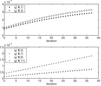
This closed-loop system has five pairs of conjugate complex-valued eigenvalues and one real-valued eigenvalue. Using the method developed in section 3.1, the single-pole peak for each eigenvalue is computed, and they are
⎡ ⎢ ⎢ ⎢ ⎢ ⎢ ⎣ ρ1,2 ρ3,4 ρ5,6 ρ7,8 ρ9,10 ρ11 ⎤ ⎥ ⎥ ⎥ ⎥ ⎥ ⎦ = ⎡ ⎢ ⎢ ⎢ ⎢ ⎢ ⎣
2.5072e−3 2.1295e−3 6.7344e−6 2.8586e−3 3.0832e−3 4.3181e−3
0 5 10 15 20 25 30 35 40 0
1 2 3 4x 10
–4
iteration
g( X,1)
g( X,3)
0 5 10 15 20 25 30 35 40 0
0.5 1 1.5 2 2.5x 10
–5
iteration
g( X,5)
g( X,7)
g( X,9)
g( X,11)
Fig. 2.The values ofg(X, k)in each iteration of the algorithm for Example1.
Obviously, the minimum value of all theρk’s isρ5 (orρ6). Therefore,k = 5 and the corresponding matricesQ,H, and Fin the set (44) are given by
Q= ⎡ ⎢ ⎢ ⎢ ⎢ ⎢ ⎢ ⎣
−6.6011e−2 −8.4915e−2 −4.3670e−1
−3.7006e−1 −4.3518e−1 −4.9156e−1
−5.0566e−1 −3.8025e−1 7.1063e−1
−5.2127e−1 −8.6900e−2 −2.2452e−1
−4.5786e−1 3.1775e−1 −1.0190e−1
−3.4878e−1 7.4183e−1 4.3249e−2
−5.1206e−1 −5.2972e−1 −5.0490e−1
−2.2314e−1 1.7033e−1 5.9434e−1
−2.5387e−1 −1.6560e−1 −5.3367e−2 7.4814e−1 −2.4759e−1 −2.2204e−1
−2.0850e−1 6.8322e−1 −4.1079e−1
−1.4270e−1 −3.6725e−1 4.1345e−1 ⎤ ⎥ ⎥ ⎥ ⎥ ⎥ ⎥ ⎦
,
H=
2.6322e+ 0 −3.9258e+ 2
−3.9258e+ 2 6.9856e+ 6
, F=
⎡ ⎢ ⎢ ⎣
4.8432e+ 4 −8.8104e+ 8
−5.2079e+ 4 9.4682e+ 8 2.4998e+ 4 −4.5374e+ 8
−2.4644e+ 4 4.4816e+ 8 ⎤ ⎥ ⎥ ⎦.
[image:15.612.95.419.101.377.2]controller realization is found, since at this iteration the conditions of Theorem 3 are met and the algorithm terminates. The resulting matrixΩopt is
Ωopt = ⎡ ⎢ ⎢ ⎣
2.3184e+ 0 −1.6411e+ 0 5.5681e−1 −7.6953e−1
−1.6411e+ 0 2.4047e+ 0 −8.2094e−1 7.0079e−1 5.5680e−1 −8.2095e−1 1.2097e+ 0 −3.7643e−1
−7.6954e−1 7.0078e−1 −3.7643e−1 1.3454e+ 0 ⎤ ⎥ ⎥ ⎦
and the corresponding global optimal transformation matrix is
Topt = ⎡ ⎢ ⎢ ⎢ ⎢ ⎢ ⎢ ⎣
−6.9470e+ 1 −3.2765e+ 4 −7.8507e−2 3.0977e+ 2 1.5431e+ 5 −1.1360e+ 0
−6.0267e+ 2 −3.0945e+ 5 2.0130e+ 0 6.5537e+ 2 3.4747e+ 5 −1.7153e+ 0
−4.1530e+ 2 −2.2683e+ 5 8.0247e−1 1.1931e+ 2 6.9580e+ 4 −1.8821e−1
−4.3363e−1 −2.7354e−1 −5.0267e−1 5.4680e−1 −1.0820e−1 9.5739e−1
−1.6781e+ 0 4.2386e−1 −7.3423e−1 2.2151e+ 0 −9.5513e−1 4.9153e−1
−1.1829e+ 0 1.0956e+ 0 −8.7755e−1 1.7712e−1 −4.5868e−1 5.6121e−1
⎤ ⎥ ⎥ ⎥ ⎥ ⎥ ⎥ ⎦ .
Example 2. The second example is taken from [14]. In this example, m = 4, n= 10,l= 2, andq= 2, and hence it is a closed-loop system of order 14. The initial controller realizationX0 ofC(z) has been given [20]. The corresponding closed-loop transition matrix A(X0) is formed using (10), from which the eigenvalues and the eigenvectors of the ideal closed-loop system are computed. This closed-loop system has six pairs of conjugate complex-valued eigenvalues and two real-valued eigenvalues given by ⎡ ⎢ ⎢ ⎢ ⎢ ⎢ ⎢ ⎢ ⎢ ⎢ ⎣ λ1,2 λ3,4 λ5 λ6,7 λ8,9 λ10,11 λ12 λ13,14 ⎤ ⎥ ⎥ ⎥ ⎥ ⎥ ⎥ ⎥ ⎥ ⎥ ⎦ = ⎡ ⎢ ⎢ ⎢ ⎢ ⎢ ⎢ ⎢ ⎢ ⎢ ⎣
−8.4482e−1±j7.8204e−2
−3.7557e−1±j3.3602e−1 2.1624e−1
7.1567e−1±j9.6631e−3 9.2895e−1±j1.2923e−1 9.8506e−1±j7.5831e−2
8.3133e−1 8.8267e−1±j3.7235e−2
⎤ ⎥ ⎥ ⎥ ⎥ ⎥ ⎥ ⎥ ⎥ ⎥ ⎦ .
Using the method developed in section 3.1, the single-pole peaks for every eigenvalues are computed, and they are
⎡ ⎢ ⎢ ⎢ ⎢ ⎢ ⎢ ⎢ ⎢ ⎢ ⎣ ρ1,2 ρ3,4 ρ5 ρ6,7 ρ8,9 ρ10,11 ρ12 ρ13,14 ⎤ ⎥ ⎥ ⎥ ⎥ ⎥ ⎥ ⎥ ⎥ ⎥ ⎦ = ⎡ ⎢ ⎢ ⎢ ⎢ ⎢ ⎢ ⎢ ⎢ ⎢ ⎣
8.3118e−3 4.0562e−2 6.2954e−2 8.0984e−3 3.7768e−3 5.4246e−3 5.8442e−3 8.0773e−3
0 1 2 3 4 5
x 104
0 0.001 0.002 0.003 0.004 0.005 0.006 0.007 0.008 0.009 0.01
iteration
g( X,1)
g( X,3)
g( X,5)
g( X,6)
g( X,8)
g( X,10)
g( X,12)
g( X,13)
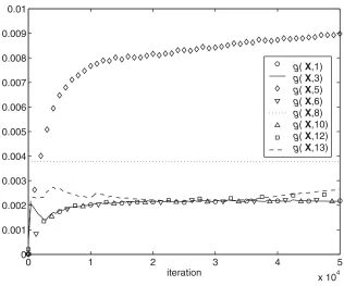
Fig. 3.The values ofg(X, k)in each iteration of the algorithm for Example2.
Obviously, the minimum value of all theρk’s isρ8 (orρ9). Therefore,k = 8 and the corresponding matrices Q,H, andFin (44) are computed according to Theorem 4. WithTin (44), the second stage of our algorithm can be executed. Figure 3 illustrates the changes ofg(X, k) in each iteration of the second stage. From Figure 3, it can be seen that after theN = 50000 iteration, we still cannot find a realization satisfying (64). This suggests that this example most likely has no saddle point (although one cannot be sure). So we terminate the algorithm at the 50000 iteration and obtain a realizationXt. Although thisXtis not an optimal realization, it is much better than X0, sincef(Xt) = 2.1539e−3 whilef(X0) = 1.1734e−4. In particular, we notice that Xt is also better than the “optimal” realization given in [14], which was found by a direct numerical optimization search using the simulated annealing algorithm and has a FWL measure value of 1.5844e−3 [14]. At this stage, we are sure that the optimal solution given in [14] is not a global optimal one at all. Using the realization Xt obtained by our search algorithm as the initial point, we then use a direct numerical optimization method to solve for the optimization problem (13) and obtain a new optimal realization whose FWL measure value is 3.1929e−3. This optimal value is more than double the one given in [14]. Obviously, we cannot tell whether or not this new optimal realization is a global optimal one. However, we know that the optimal value of the FWL realization problem for this example lies in the range of [3.1929e−3, 3.7768e−3]. For this example, no other design has found a controller realization whose FWL closed-loop stability measuref(X) is larger than 3e−3. Our algorithm is the first one to achieve af(X)>3e−3.
[image:17.612.96.412.96.359.2]Example 3. This example is a fluid power speed controller given in [8], where m= 4, n= 4,l= 1, andq= 1.
Example 4. This example is a discretized version of an H∞ robust controller
given in [26] with a sampling frequency of 250 Hz, where m= 2, n= 3, l = 1, and
q= 1.
Example 5. This example is taken from [6], where m = 3, n = 2, l = 1, and q= 1.
Example 6. This example is a steel rolling mill proportional-integral-derivative
controller given in [8], wherem= 3,n= 2, l= 1, andq= 1.
As mentioned previously, the realizations ofC(z) are not unique. For instance, in Example 1, the initially designed controller (A0
C,B 0 C,C
0 C,D
0
C) is the controllable companion-form realization for
C(z) =0.046z
6+ 0.0159z5−0.4284z4+ 0.9227z3−1.0043z2+ 0.5983z−0.1503
z6−4.26z5+ 8.2537z4−9.441z3+ 6.6649z2−2.6885z+ 0.4709 .
Apart from the controllable companion form, denoted asXc, a controller is also often implemented in the parallel or series form in practice. Denote these two realizations ofC(z) as
Xp=
DpC CpC BpC ApC (65)
and
Xs=
Ds C CsC Bs
C AsC
,
(66)
respectively. The parallel-form realization ofC(z) for Example 1 is given by
C(z) = 0.046 + 1.8921e−7
z−1 +
−0.0024z+ 0.0013
z2−0.9670z+ 0.9589
+ 0.1056z−0.1487
z2−1.6016z+ 0.7103+
0.1087
z−0.6913
with
ApC= ⎡ ⎢ ⎢ ⎢ ⎢ ⎢ ⎢ ⎣
1 0 0 0 0 0
0 0 1 0 0 0
0 −9.5886e−1 9.6700e−1 0 0 0
0 0 0 0 1 0
0 0 0 −7.1030e−1 1.6016e0 0
0 0 0 0 0 6.9134e−1
⎤ ⎥ ⎥ ⎥ ⎥ ⎥ ⎥ ⎦
,
BpC=1 0 1 0 1 1T, DpC =4.6000e−2,
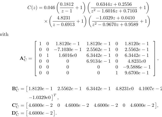
while the series-form realization is
C(z) = 0.046 &
0.1812
z−1 + 1 ' &
0.6344z+ 0.2556
z2−1.6016z+ 0.7103+ 1 '
×
&
4.8231
z−0.6913+ 1 ' &
−1.0329z+ 0.0410
z2−0.9670z+ 0.9589+ 1 '
with
AsC= ⎡ ⎢ ⎢ ⎢ ⎢ ⎢ ⎢ ⎣
1 0 1.8120e−1 1.8120e−1 0 1.8120e−1 0 0 −7.1030e−1 2.5562e−1 0 2.5562e−1 0 1 1.6016e0 6.3442e−1 0 6.3442e−1 0 0 0 6.9134e−1 0 4.8231e0 0 0 0 0 0 −9.5886e−1 0 0 0 0 1 9.6700e−1
⎤ ⎥ ⎥ ⎥ ⎥ ⎥ ⎥ ⎦
,
BsC=1.8120e−1 2.5562e−1 6.3442e−1 4.8231e0 4.1007e−2
−1.0329e0T,
CsC=4.6000e−2 0 4.6000e−2 4.6000e−2 0 4.6000e−2,
DsC=
4.6000e−2.
The above three realizations, Xc, Xp, and Xs, are sparse because they contain many trivial parameters (0, 1, or−1). For Example 1,X0 has 13 nontrivial parame-ters, whileXp andXs have only 12 nontrivial parameters (the repeated values, such as 1.8120e−1 inXs, are counted as one nontrivial parameter). Clearly, a trivial pa-rameter requires no arithmetic operation in a fixed-point implementation and does not cause any computational error. A sparse controller realization has computational ad-vantages in practical implementations. An FWL closed-loop stability measure, which is similar to the one defined in (11) but takes into account the sparsity of controller realization, is defined in [9] as
fsp(X)= min k∈{1,...,m+n}
1− |λk(A(X))| (
Ns i,j
δ(xij) ∂λk(A(X)) ∂xij
2, (67)
where
δ(xij) =
1, xij is nontrivial, 0, xij is trivial, (68)
and Ns is the number of nontrivial parameters in X. Comparing the definitions of
fsp(X) andf(X), it follows that
fsp(X)≥f(X).
[image:19.612.74.406.113.353.2](69)
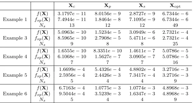
Table 1
Comparison of performance measures for different realizations.
Xc Xp Xs Xopt
f(X) 3.1797e−11 8.0156e−9 2.8727e−9 6.7344e−6 Example 1 fsp(X) 7.4944e−11 1.8464e−8 7.1095e−9 6.7344e−6
Ns 13 12 12 49
f(X) 5.0963e−10 1.5234e−5 3.0949e−6 2.7321e−4 Example 3 fsp(X) 8.5965e−10 2.7908e−5 5.4711e−6 2.7321e−4
Ns 9 8 8 25
f(X) 1.6555e−10 8.3351e−10 1.4611e−7 5.0786e−5 Example 4 fsp(X) 6.1068e−10 1.5627e−7 3.0905e−7 5.0786e−5
Ns 7 7 7 16
f(X) 1.6699e−4 5.4326e−4 4.8802e−4 3.2716e−3 Example 5 fsp(X) 2.5956e−4 2.4426e−3 7.3417e−4 3.2716e−3
Ns 5 4 4 9
f(X) 6.7163e−4 1.0775e−3 1.0774e−3 4.8968e−3 Example 6 fsp(X) 9.5044e−4 3.5239e−3 1.6347e−3 4.8968e−3
Ns 5 4 4 9
closed-loop stability robustness as measured by either f(X) or fsp(X), compared with the other three realizations. It can also be seen that the optimal realization obtained by the proposed search algorithm is a fully parameterized nonsparse one. The other three sparse realizations have similar numbers of nontrivial parameters, and thus have the same lighter computational load than that of the optimal one given here. However, it is worth pointing out thatXopt is not unique sinceVin (43) is an arbitrary orthogonal matrix. By choosingVin an appropriate way, one can obtain a sparse optimal realizationXopt. The topic of how to makeXopt sparse is beyond the scope of this paper, and interested readers are referred to the work [1] for details.
6. Conclusions. We have developed an efficient search algorithm for solving the class of optimal FWL controller realization problems based on the Frobenius-norm pole sensitivity measure, which have saddle points. Our approach first constructs the closed form of a transformation matrix set which contains global optimal solutions and then searches this set with a subgradient routine to find a global optimal solu-tion. The proposed algorithm has considerable advantages over using direct numerical optimization methods to tackle this class of optimal FWL realization problems. In particular, when the subgradient routine converges to a solution, it is guaranteed to be a global optimal solution. It has been conjectured with some empirical support that for many practical control systems the assumption of having saddle points is a valid one and the cases of optimal FWL controller realization problems which do not have saddle points are less common. It has been demonstrated that for this smaller class of optimal FWL realization problems without saddle points our algorithm also provides useful information to help solve them.
Appendix. Proof of Theorem 4. We present the proof for Case 2. The proof for Case 3 is similar and hence is omitted.
Lemma 3 (see [21]). Let real-valued matricesM22,M21, and M11>0 be given
with appropriate dimensions. Then
M11 MT21
M21 M22
>0 (70)
Lemma 4. Given positive α, β ∈ R, p,y ∈ Cn, and for any nonsingular T ∈ Rn×n, we have
ξ(T, α, β,p,y)≥(|yHp|+αβ)2.
(71)
The equality occurs if and only if there exist W ∈ Rn×n, W >0, and θ ∈ [0,2π)
satisfying
WΥ(y) =β
αΥ(p)
cosθ sinθ −sinθ cosθ
.
(72)
When(72)has solutions, the equality in(71)occurs only at the transformation matrix
T=W1/2V, whereV∈ Rn×n is an arbitrary orthogonal matrix. Proof. First,
T−1p2FTTy2F+α2TTy2F +β2T−1p2F+α2β2 (73)
≥(T−1pFTTyF+αβ)2.
The equality holds if and only if
αTTyF =βT−1pF. (74)
Using the Cauchy–Schwarz inequality, we have
(T−1pFTTyF+αβ)2≥((TTy)HT−1pF+αβ)2≥(|yHp|+αβ)2. (75)
The equality holds if and only if
TTy=cT−1p (76)
for some complex numberc.
To achieve (73) and (75) with equality, one needs to satisfy both of the conditions (74) and (76). This implies thatc= (cosθ+jsinθ)βα andθ∈[0,2π). Thus,
TTy= (cosθ+jsinθ)β
αT −1
p.
(77)
AsTis nonsingular, equality (77) is equivalent to
Wy= (cosθ+jsinθ)β
αp
(78)
with W>0 and T=W1/2V. Noticing the map Υ defined in (31), condition (78) can be viewed as
WΥ(y) =β
αΥ(p)
cosθ sinθ −sinθ cosθ
.
(79)
This completes the proof.
Lemma 5. Given positive α, β ∈ R, p,y ∈ Cn, and rank(Υ(y)) = 2, (79) has
solutions if and only ifdet((Υ(y))TΥ(p))>0. Moreover, any solution to(79)can be
expressed as
tanθ= a21−a12
a11+a22
a11cosθ−a12sinθ >0
W=Q
H FT
F G
QT
⎫ ⎪ ⎪ ⎪ ⎪ ⎪ ⎬ ⎪ ⎪ ⎪ ⎪ ⎪ ⎭
,
where
a11 a12
a21 a22
= (Υ(y))TΥ(p); (81)
the orthogonal matrixQcan be obtained from the QR factorization of Υ(y), that is,
Υ(y) =Q
γ11 0 0 · · · 0
γ12 γ22 0 · · · 0 T
; (82)
H andFare determined by
H= β
α
γ11 γ12 0 γ22
−T
(Υ(y))TΥ(p)
cosθ sinθ −sinθ cosθ
γ11 γ12 0 γ22
−1
,
(83)
F= β
α
⎡ ⎢ ⎣
eT 3
.. .
eT n
⎤ ⎥
⎦QTΥ(p)
cosθ sinθ −sinθ cosθ
γ11 γ12 0 γ22
−1 ; (84)
andGis given as
G=FH−1FT+U (85)
withU∈ R(n−2)×(n−2) being an arbitrary positive definite matrix.
Proof. If det((Υ(y))TΥ(p))>0, it is easy to verify thatWandθgiven by (80)– (85) are a solution to (79). If, on the other hand, (79) has a solutionWandθ, it can be seen that
(Υ(y))TWΥ(y) =β
α(Υ(y))
T Υ(p)
cosθ sinθ −sinθ cosθ
.
(86)
On account of (Υ(y))TWΥ(y)>0, we have
(Υ(y))TΥ(p)
cosθ sinθ −sinθ cosθ
>0.
(87)
A necessary condition to satisfy (87) is that
det &
(Υ(y))TΥ(p)
cosθ sinθ −sinθ cosθ
'
>0.
(88)
Since the left side of the above inequality is equal to det((Υ(y))TΥ(p)), the condition (88) becomes det((Υ(y))TΥ(p))> 0. This completes the proof of the first part of Lemma 5.
Now, when (81) is given, (87) holds if and only if all of the following three condi-tions are satisfied:
a21cosθ−a22sinθ=a11sinθ+a12cosθ
a11cosθ−a12sinθ >0 det((Υ(y))TΥ(p))>0
⎫ ⎬ ⎭. (89)
From the first line of (89), we directly obtain tanθ= a21−a12
a11+a22. Denote
S=QTWQ.