Flow of evaporating, gravity-driven thin liquid films over topography

This is a repository copy of Flow of evaporating, gravity-driven thin liquid films over topography.

White Rose Research Online URL for this paper: http://eprints.whiterose.ac.uk/1783/

Article:

Gaskell, P.H., Jimack, P.K., Sellier, M. et al. (1 more author) (2006) Flow of evaporating, gravity-driven thin liquid films over topography. Physics of Fluids, 18 (Art. N). 14 pages. ISSN 1070-6631

https://doi.org/10.1063/1.2148993

[email protected] Reuse

See Attached

Takedown

If you consider content in White Rose Research Online to be in breach of UK law, please notify us by

White Rose Consortium ePrints Repository

This is an author produced version of a paper published in Physics of Fluids.

White Rose Repository URL for this paper: http://eprints.whiterose.ac.uk/1783/

Published paper

Gaskell, P.H., Jimack, P.K., Sellier, M. and Thompson, H.M. (2006) Flow of evaporating, gravity-driven thin liquid films over topography. Physics of Fluids, 18 (Art. No. 013601).

Flow of evaporating, gravity-driven thin liquid films over topography

by

P.H. Gaskella, P.K. Jimackb, M. Selliercand H.M Thompsona

a_{School of Mechanical Engineering}

b_{School of Computing}

The University of Leeds, Leeds LS2 9JT, UK

c_{Fraunhofer-Institut fuer Techno- und Wirtschaftsmathematik}

Gottlieb-Daimler-Strasse, Geb. 49, 67 663 Kaiserslautern, Germany

Abstract

The effect of topography on the free surface and solvent concentration profiles of an evaporating thin film

of liquid flowing down an inclined plane is considered. The liquid is assumed to be composed of a resin

dissolved in a volatile solvent with the associated solvent concentration equation derived on the basis of the

well-mixed approximation. The dynamics of the film is formulated as a lubrication approximation and the

effect of a composition-dependent viscosity is included in the model. The resulting time-dependent,

non-linear, coupled set of governing equations is solved using a Full Approximation Storage multigrid method.

The approach is first validated against a closed-form analytical solution for the case of a gravity-driven,

evaporating thin film flowing down a flat substrate. Analysis of the results for a range of topography shapes

reveal that while a full-width, spanwise topography such as a step-up or a step-down does not appear to

affect the composition of the film, the same is no longer true for the case of localised topography, such as

a peak or a trough, for which clear non-uniformities of the solvent concentration profile can be observed

in the wake of the topography.

I Introduction

Several industrial processes require thin films to flow, under the action of body forces, over substrates

with topographic features caused, for example, either by direct patterning or by defects in the substrate.

Typical examples include paints or photoresist films, used in the lithographic stages of the manufacture of

microelectronic components1. Such flows have received considerable attention in the literature, the focus

until recently having been primarily on flow over one-dimensional topographies. Several such studies, see

for example2−4, have investigated the effect of the topography and governing parameters on continuous

thin films over combinations of step-down and step-up topographies, with particular emphasis on the

formation and stability of the Capillary ridge located just upstream of a step-down topography. These

analyses have since been extended to consider the effect of inertia and intermolecular forces5 and to

consider the motion of discontinuous thin films with contact lines over substrates containing trench or

wedge topographies6.

Due to the formidable experimental and theoretical challenges involved, fully three-dimensional flow over

topography has received far less attention in the literature to date. Hayes, O’Brien & Lammers7, for

example, formulated a Green’s function approach which enables the free surface to be calculated

success-fully for flows over shallow, arbitrary topographies, while Bielarz & Kalliadasis5employed the popular

alternating direction implicit time-splitting approach used by Schwartz and co-workers8−9 to solve for

the flow over a square mound. In contrast, Gaskell et al10 developed a Multigrid approach with adaptive

time-stepping for the efficient numerical solution of the nonlinear lubrication equations as an alternative

to time-splitting and used it successfully to solve the problems of droplet spreading on a surface with a

well-defined topography and the flow of continuous, thin water films down an inclined plane containing

a range of topographies11. The latter had recently been investigated experimentally using phase-stepped

interferometry by Decr´e and Baret1.

A detailed comparison between experiment and Finite Element solutions of the full Navier-Stokes

equa-tions for one-dimensional topographies11 has quantified the accuracy of the lubrication approach and

shown the solution of the governing equations to be accurate even when the assumptions on which they

are based are not strictly satisfied. Multigrid solutions to fully three-dimensional flows are also found to

a localised topography, can be well-represented by an inverse hyperbolic cosine function. The simulations

similarly supported the experimental findings that the free surface response for shallow topographies is

approximately linear.

Although the above studies on flow past topographies have assumed that the liquids are pure substances, in

many practical situations the liquid is composed of a functional resin dissolved in a volatile solvent. The

latter, when subsequently evaporated, leaves a solid resin film on the substrate9. The motivation therefore

of the present work is to study how flow past topography is affected by solvent evaporation and, in turn,

how the topography affects the composition of the resin/solvent mixture.

Despite few previous studies on evaporative flow over topography having appeared in the literature, such

flows over flat or curved substrates have been widely investigated, revealing a range of interesting

phenom-ena. Overdiep’s experiments12, for example, showed that the free surface of some solvent-based high-gloss

alkyd paints unexpectedly undergo reversal after the levelling of disturbances; that is, initial peaks in the

free surface become troughs and vice versa. This phenomenon was later analysed theoretically by Eres et

al13who solved a three-dimensional lubrication model of the flow numerically and confirmed that reversal

is caused by the solutal Marangoni effect due to variations in solvent concentration which in turn lead to

surface tension gradients. The latter study was one of several by Schwartz and co-workers who have

mod-elled the effects of solvent evaporation in applications ranging from the role of surface tension gradients

in correcting corner defects14 and in crater formation15, to the effect of viscosity increase due to solvent

depletion on droplet reticulation9.

Other studies of flow over planar substrates of relevance to the present work include the recent analysis of

evaporation in gravity-driven flow of a discontinuous, thin liquid film with a dynamic contact line16and, in

particular, that of Meyerhofer17 which is credited as being the first attempt to model the effects of solvent

evaporation and the associated viscosity rise on the thickness of dried films during spin coating. Using a

one-dimensional, axisymmetric model for film thickness and solvent concentration, he proposed that film

thinning in spin coating occurs in two distinct stages. At first, the effect of evaporation is negligible and

the film thins mainly by centrifugally-driven flow toward the edge of the substrate. During the second

stage, solvent evaporation becomes the dominant mechanism for film thinning as the viscosity rise due to

Meyerhofer’s model was subsequently extended to consider the effects of solvent concentration across the

film18, although still in the context of a one-dimensional analysis. The two-stage assumption of

Meyer-hofer was later used by Stillwagon and Larson19in a lubrication analysis to predict the free surface profile

of a drying spin coated film over topography. Their model for the initial, flow-dominated stage was unable

to predict how the topography affects the solvent concentration and, the excellent agreement between their

theory and experiment showed that such effects are small in the context of spin coating.

The present study similarly focuses on the initial stages of the flow during which the viscosity increases due

to solvent concentration, but in the different context of constant flux gravity-driven flow of a continuous,

thin film down an inclined plane with topography. The flow is clearly different from that of

centrifugally-driven flow but the mathematical framework in the context of the lubrication approximation differs only

in terms of the nature of a dimensionless number - see eq. (5) of reference 19. This follows in that for

spin coating it is customary to: (i) ignore the axisymmetry of the flow if a topography is sufficiently far

from the axis of symmetry; (ii) adopt a quasi-steady analysis by treating the flux as constant since the

rearrangement of fluid over a topography occurs much faster than any associated film thinning due to the

presence of a non-constant flux - see also references 20 and 21.

Section 2 describes the flow under consideration together with the analytical and numerical lubrication

models, both of which employ the assumption that the resin and solvent are well-mixed. A brief overview

of the solution methodology then follows since a detailed description of the multigrid approach on which it

is based is already available10. Results, in ascending order of complexity, then follow. First, the analytical

solution for the two-dimensional flow (i.e. invariant in the spanwise direction) of an evaporating thin

liquid film down a flat inclined plane is derived, following on from Huppert’s earlier analytical solution

for the non-evaporating case22. This analysis reveals that the free surface can exhibit three distinct types of

behaviour, dependant on the evaporation rate and how steeply viscosity increases with evaporative solvent

loss. This analytical solution provides a convenient reference by which to assess the effect of a step-down

and a trench topography on the solvent concentration and is used to validate the numerical predictions.

Results for the fully three-dimensional flow of an evaporating film down an inclined plane over localised

II Problem formulation

In the context of thin liquid films the fact that the ratio ε= H0

L is small, where H0 is the characteristic

film thickness and L the characteristic length in the streamwise direction, can be exploited to reduce the

general governing Navier-Stokes equations to a more tractable coupled pair of second order nonlinear

partial differential equations in terms of the film thickness, H, and the pressure across the film, P. This

approach, commonly referred to as the lubrication or long-wave approximation, has been used successfully

by a number of authors to model a variety of thin film flows23. For the particular case of gravity-driven,

non-evaporative flow over topographies its accuracy has recently been quantified11.

A. Governing Equations

The case of flow of a continuous film of liquid, of constant flux Q0, over a surface (lateral extent L and

span width W ) containing distinct topographic features and inclined at an angle α to the horizontal is

illustrated in Figure 1, which shows the notation adopted and the accompanying coordinate system. Each

well-defined topographical feature has amplitude S0 and form S(X,Y), with lateral extent LT and span

width WT, centred at (XT,YT). These features may completely span the domain (in which case WT =W

and LT ≪L, leading to two-dimensional flow), or be localised (i.e. WT ≪W and LT ≪L, giving

three-dimensional flow). Each topography may either be a depression (S0<0) or a protrusion (S0>0).

The liquid is assumed incompressible and Newtonian, with constant densityρand surface tensionσ. The

solvent concentration cs=hs/h is defined by the ratio of the imaginary thickness of the solvent layer, hs,

to the total film thickness h13 and, following previous studies9,13,14, the viscosity µ is assumed to depend

exponentially on cs, obeying:

µ=µ0ea(c0−cs), (1)

where µ0 is the reference value of the concentration-dependent dynamic viscosity and c0 is the initial

solvent concentration. The parameter a controls the sensitivity of the viscosity to solvent concentration

variations; its form ensures that the viscosity effectively precludes flow for small solvent concentrations.

thickness is that commensurate with fully developed film flow11, viz

H0=

3µ0Q0 ρg sinα

1/3

, (2)

while the extent of the substrate, L, is equal toβtimes the dynamic capillary length, Ld, viz:

L=βLd where Ld=

σH0

3ρg sinα

1/3

= H0

6Ca1/3 . (3)

Here, Ca=µ0U0

σ , is the Capillary number expressing the ratio of viscous to surface tension stresses. Unless

otherwise stated,βis chosen to be equal to 50, a large enough value to ensure that the free surface relaxes

to its undisturbed shape downstream of the topography.

The characteristic velocity U0is taken to be the free surface velocity of the fully developed film, namely:

U0=

3Q0

2H0

, (4)

while the characteristic pressure and time scale are P0= ρgL sin₂ α and T0=_UL₀, respectively.

Based upon these scalings, the following dimensionless variables:

h(x,y,t) = H

H0

, s(x,y) = S

H0

, ˜µ = µ

µ0

, (x,y) = (X,Y)

L , (5)

z = Z

H0

, p(x,y,t) = P

P0

, (u,v,εw) = (U,V,W) 1

U0

, t = T

T0

,

when introduced into the Navier-Stokes equations, and retaining leading-order terms (those up to O(ε2_,ε2_Re))

yields the following mass conservation equation:

∂h

∂t +∇.Q+e=0, (6)

where e=E/(εU0) is the constant, dimensionless, evaporation rate and the flux vector Q is defined as

(Qx,Qy)T = Rh+s

s (u,v)T dz. The evaporation rate E has the dimensions of a velocity (the rate of thinning

of a flat film) and is chosen to be constant since only small variations of the solvent concentration are

power law proposed in Schwartz et al9.

Applying a no-slip boundary condition at the surface of the solid substrate and assuming negligible shear

stress at the liquid-air interface yields:

Qx = −

h3

3˜µ

∂p

∂x −2

, (7)

Qy = −

h3 3˜µ ∂p ∂y , (8)

which, when combined with equation (6), gives

∂h

∂t =

∂ ∂x h3 3˜µ ∂p

∂x−2 + ∂ ∂y h3 3˜µ ∂p ∂y

−e. (9)

The pressure across the film results from contributions from the surface tension and the hydrostatic

pres-sure:

p=− 6

β3∇

2_{(h+s) +}2 β6

1/3_{N(h+s), (10)}

where∇2_{(h+s)is the small slope approximation to the free surface curvature and N =Ca}1/3_cotα

mea-sures the relative importance of the normal component of gravity24.

As pointed out by Howison et al25, one of the key parameters dictating the choice of evaporation model is

the diffusivity of the solvent. If the diffusion of solvent is sufficiently rapid, the leading-order distribution

of solvent across the film is uniform, leading to the so-called well-mixed assumption9. This assumption

fits naturally within the lubrication formalism for which all quantities are depth averaged and has been

used successfully to predict the formation of defects in drying films9,15. If the well-mixed assumption is

violated, variations of the solvent concentration across the film have to be taken into account and it is

not possible to remain within the framework of the lubrication approximation unless the fluid parameters

(viscosity, surface tension) are assumed constant across the film26. Howison et al25 discussed the validity

of the well-mixed approximation and showed it to be valid provided the characteristic time for the solvent

to diffuse across the film, t_dacross=H₀2/D, is much smaller than that for the fluid to flow across the film,

for solvent conservation is given by

∂(hcs)

∂t +∇.

csQ=−e+d∇.(h∇cs) , (11)

where d=D/LU0 is the dimensionless solvent diffusivity. Combining equation (11) with equations (6),

(7) and (8) yields:

∂cs

∂t =

h2

3˜µ

∂p

∂x −2

∂cs

∂x + h2 3˜µ ∂p ∂y

∂cs

∂y +e

(cs−1)

h +

d

h∇.(h∇cs) , (12)

where ˜µ=µ/µ0 is the viscosity ratio at a given solvent concentration. Howison et al25 showed also that

the lateral diffusion in equations (11) and (12) is dominated by convection provided D≪LU0, in which

case equation (12) reduces to:

∂cs

∂t =

h2

3˜µ

∂p

∂x −2

∂cs

∂x + h2 3˜µ ∂p ∂y

∂cs

∂y +e

(cs−1)

h . (13)

Before discussing appropriate boundary conditions for the evolution equations (9), (10) and (13), their

validity for the results presented below is assessed by considering a realistic example. In Table 1,

repre-sentative solvent/resin properties9,25 have been used to calculate maximum and minimum values for the

associated scalings and dimensionless groups for the case of a 70 µm thick film flowing down a plane

inclined at 30oto the horizontal with physical properties in the ranges 0.001Pas≤µ≤0.5Pas, 0.02Nm−1

≤σ≤0.05Nm−1, 10−8 ms−1≤E≤10−6 ms−1, and 10−9 m2s−1 ≤D≤10−7 m2s−1 and with a

sub-strate that extends over 50 Capillary lengths(β=50). Note that in practice D is a strongly varying function

of solvent concentration which may change by several orders of magnitude as the solvent concentration

varies25.

As discussed above, the twin assumptions that the solvent is well-mixed and that lateral diffusion is

negli-gible, required to obtain equation (13), are valid providedε2_{≪d≪1; Table 1 shows that this condition is}

met except for thick films with very small viscosity and diffusivity. All subsequent results employ the data

set: µ0=0.025 Pa s,ρ=1000 kg m−3,σ=0.035 N m−1, D=10−8m2s−1and 10−8m s−1≤E≤10−6

m s−1(i.e. 0.008≤e≤0.8). The corresponding scalings and dimensionless groups used in the

Consider now the assumption used in deriving equation (9) that the surface tension is constant. According

to Howison et al25 the characteristic in plane velocity for flows driven by surface tension gradients is

Ug= ε∆c_µs₀∆σ, where∆cs denotes a characteristic measure of the variation in solvent concentration and∆σ

the difference between the surface tension of pure resin and that of pure solvent. Since ∆σ is usually

O(10−2)and∆csis also O(10−2), Table 1 also shows that for the results presented below, Ug≪U0so that

Marangoni effects can indeed be neglected.

B. Boundary and initial conditions

At the upstream boundary, x=0, the assumption of fully developed flow yields

h(x=0,y) =1, cs(x=0,y) =c0 and ∂p

∂x(x=0,y) =0. (14)

Along the streamwise boundaries, y=0 and y=1, the spanwise gradients in h and p are zero to impose

zero spanwise flux. Since solvent depletion causes film thickening due to the associated increases in

viscosity, at the downstream boundary, x=1, the conditions there are chosen to allow a non-zero free

surface slope:

∂2_h

∂x2(x=1,y) = ∂p

∂x(x=1,y) =0. (15)

Initially, the free surface is prescribed to be flat (h(x,y,t =0) +s(x,y) =1) with a uniform solvent

con-centration c0, although the specific choice of initial conditions is found to be unimportant in practice since

the same steady-state is reached for all initial conditions tried.

Equations (6), (10) and (13) constitute the governing equations for the dependent unknowns h(x,y,t),

p(x,y,t)and cs(x,y,t)and these are fully defined for specific values of a, c0, β, N and e. The numerical

scheme for solving them is based on the

F A S

in-terested reader is directed to the pioneering work of Brandt27,28for an in depth overview of the method and

III Method of solution

Solutions are sought on a square computational domain with (x,y)∈Ω= (0,1)×(0,1) and a uniform

mesh having (2kf _{+1) nodes in each direction. The discrete analogue of eqs. (6), (10) and (13) are}

obtained using central differences, leading to the following second order accurate spatial discretisations

∂hi,j

∂t =

1

∆2

h3

3˜µ|i+12,j

pi+1,j−pi,j

−h

3

3˜µ|i−12,j

pi,j−pi−1,j

+

h3

3˜µ|i,j+12

pi,j+1−pi,j− h3

3˜µ|i,j−12

pi,j−pi,j−1

−

2h2_i,j

hi+1,j−hi−1,j

2∆

−e+O(∆2), (16)

pi,j+

6

β3_∆2

(hi+1,j+si+1,j) + (hi−1,j+si−1,j) + (hi,j+1+si,j+1) +

(hi,j−1+si,j−1)−4(hi,j+si,j)

−2

β6 1/3_N(h

i,j+si,j) +O(∆2) =0, (17)

∂c_si,j

∂t =

h2_i,j

12˜µi,j∆2

pi+1,j−pi−1,jcsi+1,j−csi−1,j

+

pi,j+1−pi,j−1csi,j+1−csi,j−1

− h

2

i,j

3˜µi,j∆

c_si+1,j−c_si−1,j+

e

c_si,j−1

hi,j

+O(∆2), (18)

for any interior point (i,j) in the computational domain, where ∆=2−kf _{is the spatial increment. The}

mid-point interpolation of the prefactorsΓ(h) = h_3˜µ3 in eq. (16) simply consists of a linear interpolation of

the prefactor between the two neighbouring nodes, viz

h3

3˜µ|i±12,j=

1 2

h3

3˜µ|i±1,j+

h3

3˜µ|i,j

, (19)

with analogous expressions for h_3˜µ3|_i,j±1 2.

derivatives in eqs. (16) and (18). The implicit nature of the scheme ensures the stability of the time

integration. Accordingly, eqs. (16) and (18) are rewritten as follows,

hn_i,+_j1−1

2∆t

n+1_Fn+1 _{= h}n i,j+

1 2∆t

n+1_Fn_{, (20)}

csn_i,+_j1−

1 2∆t

n+1_Gn+1 _{= c}

sni,j+

1 2∆t

n+1_Gn_{, (21)}

where Fn and Gn correspond respectively to the right-hand side of eqs. (16) and (18) (excluding the

remainder terms) at the nth time step. Consequently, at each time step it is necessary to solve the coupled

nonlinear system given by equations (20), (17) and (21) at each grid point(i,j). This may be written in

the following condensed form:

Lh_kf hn_k+1

f ,p

n+1

kf ,cs

n+1

kf

= f_kh_f hn_kf,pn kf,cs

n kf

, (22)

L_kp

f h

n+1

kf ,p

n+1

kf

= 0, (23)

Lcs

kf h

n+1

kf ,p

n+1

kf ,cs

n+1

kf

= fcs

kf h

n kf,p

n kf,cs

n kf

, (24)

where f_kh

f and f

cs

kf correspond to the right-hand side of eqs. (20) and (21) respectively.

The solution scheme employed for this large algebraic system is based upon a straightforward

general-ization of the multigrid procedure described in Gaskell et al10. This multigrid algorithm requires a small

number of iterations of a nonlinear Gauss-Seidel solver to be taken on the finest grid, with(2kf_+1)nodes

in each direction, and then both this “pre-smoothed” solution and the corresponding residuals are restricted

to a coarser grid. A “coarse grid correction” problem is then solved on this mesh and the computed

correc-tions to h, p and csare interpolated back to the fine mesh. The latest fine grid solution is then updated and a

small number of further Gauss-Seidel iterations are taken (the “post-smooths”). Note that the coarser grid

problem may itself be solved by the same process of taking a small number of pre-smooths, a still coarser

grid correction and then some post smooths. At the coarsest grid encountered a different solution

proce-dure is required; for this work (unlike in Gaskell et al10) simply a large number of nonlinear Gauss-Seidel

iterations are used, leading to satisfactory solutions provided the grid is sufficiently coarse (e.g. 9 nodes in

each direction). This whole process is referred to as a single V-cycle and may be repeated numerous times

In order to describe the nonlinear Gauss-Seidel smoother used in this work, consider the equations that

must be solved at an arbitrary grid level, level k say. These equations always take the same form as (22) to

(24) however∆is now equal to 2−kand the coarse grid correction causes a modification to the right-hand

sides when k<kf (see Gaskell et al10or Trottenberg et al30 for full details). Hence, at each node(i,j)on

level k, these equations may be expressed as

[Lh_k hn_k+1,pn+1 k ,cs

n+1

k

]i j = [fkh]i j, (25)

[L_kp hn_k+1,pn+1 k

]i j = [f_kp]i j, (26)

[Lcs

k h

n+1

k ,p

n+1

k ,cs n+1

k

]i j = [f_kcs]i j. (27)

Given an estimate, (h0n_k+1,p0_kn+1,cs0n_k+1), to the solution of this system, the smoother then defines the

updates to this at node(i,j) to be the solution of the following 3×3 system (where all expressions are

evaluated at the latest estimate):

∂[Lh_k]i j

∂(hk)i j

∆h+ ∂[L

h k]i j

∂(pk)i j

∆p+ ∂[L

h k]i j

∂(cs,k)i j

∆cs = [fkh]i j−[Lhk]i j, (28)

∂[L_kp]i j

∂((hk)i j

∆h+∂[L

p k]i j

∂(pk)i j

∆p+ ∂[L

p k]i j

∂(cs,k)i j

∆cs = [f_kp]i j−[L_kp]i j, (29)

∂[Lcs

k ]i j

∂(hk)i j

∆h+∂[L

cs

k ]i j

∂(pk)i j

∆p+ ∂[L

cs

k ]i j

∂(cs,k)i j

∆cs = [f_kcs]i j−[Lc_ks]i j. (30)

Hence the updated approximation to the solution at point(i,j) (on grid level k) is given by: h_0i,jn+1=

h0ni,+j1+∆h, p0i,jn+1=p0ni,+j1+∆p andcs,_0i,jn+1=cs,0ni,+j1+∆cs. Furthermore this 3×3 matrix problem

that must be solved for each grid point is simplified by the fact ∂[L

p k]i j

∂(cs,k)i j =0 since the discretised pressure

equation, (26), does not explicitly depend on the solvent concentration. In all other respects the solution

procedure used here is as described in Gaskell et al10.

IV Results and discussion

Results for gravity-driven flow of continuous thin films with evaporation are presented in three

analyti-cally, before two-dimensional and three-dimensional flows over topography are investigated numerically.

Unless otherwise stated, results are for a film with H0=70µm,α=30oand the parameters listed in

Ta-ble 1, with mesh independent numerical solutions obtained on a grid extending over 50 Capillary lengths

(β=50) in the X and Y directions using a finest grid level of 257×257 (kf =8).

A. Evaporating flow over a flat substrate

The problem of a pure liquid film draining down a flat, inclined plane for the case of constant flux is

trivial in the absence of evaporation, yielding a liquid film of uniform thickness, the behaviour of which

is modified when solvent evaporation induces viscosity variations. Intuition suggests that the free surface

shape is determined by two competing effects as the fluid flows further and further downstream: thinning

due to evaporative solvent loss and thickening due to the resultant increase in viscosity. By adopting

the same assumptions as Huppert22, who investigated the fingering instability in gravity-driven thin films

down a slope, a simple analytical solution for the film thickness, solvent concentration and therefore

the viscosity can be obtained; this also provides a useful means of validating corresponding numerical

solutions. Huppert assumed that the effects of surface tension and the component of gravity normal to

the substrate could be neglected, so that the fluid motion is dictated by a balance between the tangential

component of gravity driving the liquid and viscous stresses, and derived a simple similarity solution

which describes the evolution of the free surface as a function of time. In the absence of a topography, the

free surface can only be deformed by the effects of evaporation which act on a sufficiently long wavelength

for surface tension effects to be safely neglected.

While Huppert considered the evolution of a fixed amount of liquid located at time zero at the top of an

inclined plane, a corresponding steady state analytic solution can be found for the present configuration in

which the film is fed by a constant flux at inlet. Invoking Huppert’s assumptions, equations (6) and (13)

become:

−2 d

dx

h3

3˜µ

−e = 0, (31)

−2h

2

3˜µ

dcs dx +e

(cs−1)

where partial derivatives have been replaced by ordinary derivatives in this one-dimensional analysis. The

first equation (31) simply yields

h3

3˜µ=−e

x

2+K1, (33)

while the upstream boundary conditions, h(x=0) =˜µ(x=0) =1, lead to K1=1/3.

Combining equations (32) and (33) and imposing the condition cs(x=0) =c0, yields

cs=

2

3(1−c0) ex−2

3

+1, (34)

Equation (34) reveals that at x0= 2₃c_e0 (X0= Q_E0c0 in dimensional quantities) cs =0, indicating that the

solvent has evaporated completely there, a result that simply asserts the conservation of solvent since

Q0c0 is the inlet flux of solvent and EX0is the amount of solvent lost through evaporation. Equations (1)

and (34) enable the viscosity derivative to be rewritten as

d ˜µ

dx =−a˜µ dcs

dx =a˜µe

2(1−c0)

3ex−2₃2 ,

(35)

so that differentiation of eq. (33) yields

−2h

2

e˜µ

ex−2

3

2

dh

dx =

ex−2

3 ex− 2

3(1−a(1−c0))

. (36)

The factor multiplying the film thickness derivative in equation (36) is necessarily negative and therefore

the sign of the film thickness derivative is dictated by the sign of the quadratic function on the

right-hand side. One of its roots, x1 = _3e2, can be disregarded since it lies beyond x0, the location at which

all solvent has evaporated. Depending on the value of the second root, x2 = _3e2 (1−a(1−c0)), three

different types of free surface shape can be expected. If x2≤0, the surface rises because of the increase of

viscosity as solvent evaporates; if x2≥x0, the film thickness monotonically decreases due to solvent loss

by evaporation; in the intermediate case, where 0<x2<x0, the film thins up to x=x2and then thickens

for the reasons stated above. These three forms of free surface behaviour are illustrated in Figure 2. The

values of x2 and x0, as per the figure, confirm that the behaviour of the free surface is dictated by the

value of the x2root. Note that for very large values of a, the dramatic increases in both viscosity and film

Analytical solutions for the case with e= 0.05, c0 = 0.7 and, following Schwartz et al9, a =70 are

compared with corresponding numerical results in Figure 3. An additional(x+,y+)coordinate system is

introduced for the presentation of results. This has the same origin as the(x,y)coordinate system but the

norm of the unit vector is the Capillary length, i.e. (x+,y+) =β(x,y)where L=βLd. Figure 3 shows the

profiles of film thickness, solvent concentration and viscosity obtained at different dimensionless times

(t =1, t =2 and t =4) and demonstrates that, after a transient initial stage, the film reaches a

steady-state; indeed, from t =2, onwards, the time-dependent simulation is almost indistinguishable from the

steady-state analytical solution. This good agreement between numerical and analytical solutions indicates

that, in this regime, the effects of the surface tension and hydrostatic pressure included in the numerical

simulations, but neglected in the analytical model, are indeed negligible.

B. Evaporating flow over a spanwise topography

Flows over one-dimensional topography in the absence of evaporation have been widely studied. That

over a step-up topography, for example, is known to produce a free surface depression1just upstream of

the topography, while flow over a step-down creates a Capillary ridge2before relaxation of the free surface

further downstream. Of particular interest here is examining the validity of previous studies of

evapora-tive flow during industrial spin coating17,19,31, which have assumed that the free surface profile can be

predicted by dividing the process into two stages. In the first, flow-dominated stage, the film profile is

considered to be controlled by a balance between a driving force and the capillary force within the

lubri-cation approximation, under the assumption that neither the topography nor the free surface disturbance

caused by it affect the distribution of solvent within the resin/solvent mixture. In the second, or shrinkage,

stage the film simply shrinks without flow by further evaporative drying. The transition between the two

stages if often assumed to occur abruptly at a critical solvent concentration17,19.

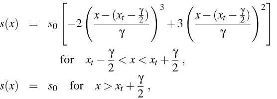
The flow over a step-up topography is considered first. Full-width topographies are defined by means of a

cubic function, bridging two regions of the substrate of different heights, as follows29:

s(x) = 0 for x<xt−

γ

s(x) = s0

⎡

⎣−2

x−(xt−₂γ)

γ

3

+3

x−(xt−γ₂)

γ

2⎤

⎦

for xt−

γ

2<x<xt+

γ

2 ,

s(x) = s0 for x>xt+

γ

2 , (37)

where γ controls the steepness of the topography. The form of equation (37) ensures that the substrate

function, s(x), is never multivalued and approximates sharp edges in the limit of γ→0. As written it

defines a step-up while a similar expression exists for a step-down; the trench considered later is simply

defined as a combination of the two.

Figure 4 shows numerical predictions of the free surface profile for flows with 0≤e≤0.05 over a step

height of s0=0.5 (half the asymptotic film thickness) withγ=0.05; the corresponding topography

pro-file is also shown. As expected, increasing the solvent evaporation rate increases the viscosity of the

resin/solvent mixture and leads to an increase in the film thickness as the mixture flows further

down-stream. The downstream viscosity increase for the e=0.05 case is also shown in Figure 4, as is the

resin/solvent interface defined by hr+s, where hr = (1−cs)h. The latter is fictitious, of course, since

the resin and solvent are assumed to be well-mixed. However, despite the obvious increase in film

thick-ness with solvent evaporation rate, the free surface profiles near the step-up are qualitatively similar, with

progressively smaller free surface depressions as the evaporation rate increases.

Figure 5 compares numerical predictions for evaporating flow over the topography of Figure 4 with the

analytical solution for the particular case of e=0.05. Although the analytical solution cannot be expected

to be valid near the topography, any significant differences between the two predictions would indicate

that the topography is having a lasting influence on the composition of the resin/solvent mixture. This

finding would contradict the assumptions of the earlier analyses of evaporating, spin coating flows cited

above17,19. In fact, the steady-state one-dimensional form of the governing equations (9) and (13)

d dx h3 3˜µ d p dx −2

−e = 0, (38)

h2

3˜µ

d p dx −2

dcs

dx +e

(cs−1)

h = 0, (39)

of the_dXdP−2terms. Eliminating _3˜µh3 d p_dx−2from equations (38) and (39) yields the following ordinary

differential equation for cs:

ex−2

3

dcs

dx +e(cs−1) =0. (40)

The solution of this equation which satisfies the condition cs=0 at x=0 is exactly the same as that found

earlier using Huppert’s assumptions, i.e. equation (34). Hence spanwise topography can have no influence

on the solvent concentration for the uniform evaporation rates considered here, while the film thickness

and pressure are affected by the exponent a in the viscosity law (1). Figure 5 confirms the independence

of solvent concentration from the topography and shows that the free surface disturbances caused by the

topography are quickly dissipated further downstream.

The next three Figures consider gravity-driven, evaporating flow over a spanwise trench-shaped

topogra-phy whose lateral extent is two Capillary lengths and with a depth of 0.7H0, i.e. s0=−0.7. Figure 6 shows

the profile of the topography, together with the computed free surface, fictitious resin/solvent interface and

viscosity ratio profiles for the case e=0.05, a=70 and c0=0.7. The free surface shows the same

fea-tures as observed in the non-evaporating case1,11, namely a Capillary ridge followed by a depression over

the trench shifted vertically, of course, due to the increasing viscosity in the downstream direction as a

consequence of evaporative solvent loss. Figure 7 compares the numerical solution given in Figure 6 with

the analytical solution for the case without any topography. Once again, the agreement is excellent with

free surface disturbances near the (large) topography quickly dissipating downstream of it.

Flow over this trench-shaped topography is now studied for a second, much larger evaporation rate (e=

0.4) in order to assess the effect of a greater streamwise variation in the solvent concentration. In Figure

8, the parameter a=2 has been chosen so that 0 <x2 =0.667<x0 =1.167 with the result that the

analysis predicts that the film will thin up to x=x2 and then thicken thereafter. The free surface exhibits

the expected features of a Capillary ridge just upstream of the trench and a depression over it and, for this

higher evaporation rate, the numerical predictions agree well with the corresponding analytical ones. In

particular, the analytical prediction that the dip in the free surface will be at x+2=βx2=33.35, agrees

well with that predicted numerically, even when the flow is over the large trench shown in Figure 6.

In summary, the assumption of earlier spin coating studies17,19,31 that spanwise topography has no effect

studied here.

C. Evaporating flow over a localised topography

The topography considered is a square trench of extent 5 Capillary lengths (lt =wt=0.1 since the

com-putational domain is 50Ld×50Ld) with a depth equal to half the asymptotic film thickness, s0=−0.5,

centred at(x_t+,y_t+) = (17.5,25.0). The topography s(x,y)is given by

s(x,y) = s0

b0

tan−1

x+−x_t+−lt/2 ltγ

+tan−1

−x++x+_t −lt/2 ltγ

×

tan−1

y+−y_t+−wt/2 ltγ

+tan−1

−y++y+_t −wt/2 ltγ

, (41)

where

b0 = 4 tan−1

1 2γ tan−1 wt/lt

2γ

. (42)

For consistency with earlier results, the topography steepness parameter,γ, is once again set equal to 0.05.

Numerical results, after reaching steady-state, are shown in Figure 9 for e=0.0 and e=0.01. The free

surface for the evaporating case ((c)) displays similar features to its non-evaporating counterpart11 (9(a)):

an upstream Capillary ridge with comet tails on each side of the topography and a downstream surge in the

middle. The pressure field for the evaporating case (9(d)) is also similar to its non-evaporating counterpart

(9(b)) with two steep peaks formed on the upstream and downstream walls of the topography separated by

a pressure drop across it. The solvent concentration field is shown in Figure 9(e). As well as the inevitable

solvent depletion in the downstream direction caused by evaporation, in contrast with two-dimensional

flows the localised topography produces a localised disturbance to the solvent concentration field which

persists in the downstream direction. The corresponding viscosity field is shown in Figure 9(f). Due to

the chosen viscosity dependence on solvent concentration, equation (1), peaks in solvent concentration

correspond to viscosity minima and vice versa.

Given the general lack of experimental data available for thin film evaporating flows a plausible

expla-nation for the spanwise variation in the solvent concentration observed in the presence of localised

solvent will be lost through evaporation at a fixed streamwise location, x. Now, since the fluid layer

cov-ering the trench is deeper than elsewhere, the resulting decrease in solvent concentration will be smallest

there; consequently, the solvent concentration immediately downstream of the topography will be greater

than its surroundings. This argument is consistent with the last term in equation (13) which tends to

de-crease the rate of change of solvent concentration where the film thickness inde-creases and vice versa. The

localised downstream ’surge’ out of the trench11 arises similarly from a corresponding mass continuity

consideration.

The above features are seen more clearly by considering spanwise profiles downstream of the topography.

Figure 10 shows the spanwise variation (0≤y+ ≤50) in film thickness, pressure, solvent concentration

and viscosity at three different spanwise locations: x+ =25, 30 and 35. The amplitudes of the film

thickness and pressure variations shown in Figures 10(a) and (b) clearly decay in the downstream direction,

together with an accompanying shift of the extrema in h and p away from the streamwise centreline,

y+ = 25. The latter leads to the characteristic ”horseshoe” shape of the Capillary wave. In contrast,

Figures 10 (c) and (d), the peak and troughs in the spanwise solvent concentration (and hence viscosity)

caused by the streamwise topography walls persist in the downstream direction. The heterogeneity in

solvent, and hence functional resin, concentration triggered by this relatively simple three-dimensional

topography may have undesirable consequences on the quality of the remaining dried film. Clearly, if all

the solvent evaporated instantaneously, these variations in resin concentration would appear as defects in

the dried film downstream of the topography. The prediction of the final dried film profile is essential from

an industrial viewpoint and constitutes a natural extension to the present work.

Decr´e and Baret1 and Gaskell et al11 found that for the non-evaporating case the free surface responds

to small topographies (|s0| ≤ 0.1) in a near-linear fashion. The final figure considers the linearity issue

for evaporating flows. Figure 11(a) shows the surface constructed by averaging the free surface for the

flow over the trench topography in Figure 9 with that over an equal but opposite topographic peak with

s0=0.5. Although the two surfaces largely cancel one another out to leave the expected approximately

uniform increase in free surface height with downstream location due to solvent depletion, as reported in

the non-evaporating case11, there are small differences in and around the topography and in the positions

of the spanwise extrema. Note, however, that these differences are small compared to the free surface

profiles through the centre of the topography, y+=25. This shows clearly that the average profile is indeed

close to that predicted for the same evaporation rate but without a topography, i.e. s0=0. Even for flow

past large topographies with s0=±0.5, for which the lubrication assumptions are not strictly valid, the

maximum difference between the two profiles is less than 2%. Table 2 presents further data on the validity,

or otherwise, of Decr´e and Baret’s assumption of a linear free surface response to topography. It shows

that, as expected, its accuracy increases rapidly as topography amplitude is reduced and that increasing

evaporation rate also has the same effect but to a lesser degree.

VI Conclusion

The flow of an evaporating thin liquid film down an inclined plane has been explored in the framework of

the lubrication and well-mixed approximations, analytically in the case of flat substrates and numerically

for flows past well defined topography.

The analytical solution to the simplified problem, when the effect of surface tension and hydrostatic

pres-sure can be neglected, provides a convenient test case. For the viscosity dependence upon solvent

concen-tration used here, equation (1), three regimes of free surface development are identified depending on the

value of x2= _3e2 (1−a(1−c0))(X2= Q_E0(1−a(1−c0))in dimensional quantities). In the first regime,

the viscosity increase caused by solvent depletion in the downstream direction causes the film to thicken

monotonically while in the second the opposite behaviour is observed: the film simply thins

monotoni-cally due to solvent loss. In the final regime the delicate balance between solvent loss and its associated

viscosity increase causes the film to thin initially before thickening further downstream when the viscosity

increase becomes dominant.

For two-dimensional evaporating flows over spanwise topography, the analysis predicts that solvent

con-centration cannot be affected by the presence of the topography and depends only on the evaporation rate

and the initial solvent concentration; film thickness and pressure do, however, depend on the particular

vis-cosity law used. Numerical predictions for two-dimensional evaporating flows over a range of spanwise

topographies are found to agree well with analytical predictions and, further, to support the assumptions

has no effect on the composition of the resin/solvent mixture. In contrast, however, the presence of a

localised topography such as a peak or trench can lead to persistent heterogeneities in the composition of

the resin/solvent mixture. In the cases studied here, flows over square trenches and peaks, the sides of the

topography can cause large local extrema in solvent concentration which could lead to unacceptable

varia-tions in the properties of the dry, functional coating. Clearly, the ability to predict the interacvaria-tions between

evaporating flows and localised topography will be of significant benefit to scientists and industrialists

alike.

Acknowledgement

The authors are grateful to Philips Electronics, Eindhoven, for sponsoring this work and to Yeaw-Chu Lee

for his helpful discussions on Multigrid methods.

References

[1] M.M.J. Decr´e, and J-C. Baret, “Gravity driven flows of viscous liquids over two-dimensional

to-pographies,” J. Fluid Mech. 487, 147 (2003).

[2] S. Kalliadasis, C. Bielarz, and G.M. Homsy, “Steady free-surface thin film flow over two-dimensional

topography,” Phys. Fluids 12, 2845 (2000).

[3] S. Kalliadasis, and G.M. Homsy, “Stability of free surface thin-film flows over topography,” J. Fluid

Mech. 448, 387 (2001).

[4] A. Mazouchi, and G.M. Homsy, “Free surface Stokes flow over topography,” Phys. Fluids 13, 2751

(2001).

[5] C. Bielarz, and S. Kalliadasis, “Time-dependent free-surface thin film flows over topography,” Phys.

Fluids 15, 2512 (2003).

[7] M. Hayes, S.B.G. O’Brien, and J.H. Lammers, “Green’s function of steady flow over a

two-dimensional topography,” Phys. Fluids 12, 2845 (2000).

[8] L.W. Schwartz, and R.R. Eley, “Simulation of droplet motion on low energy and heterogeneous

surfaces,” J. Colloid Interface Sci. 202, 173 (1998).

[9] L.W. Schwartz, R.V. Roy, R.R. Eley, and S. Petrash, “Dewetting patterns in a drying liquid film,” J.

Colloid Interface Sci. 234, 363 (2001).

[10] P.H. Gaskell, P.K. Jimack, M. Sellier, and H.M. Thompson, “Efficient and accurate time adaptive

multigrid simulations of droplet spreading,” Int. J. Numer. Meth. Fluids 45, 1161 (2004).

[11] P.H. Gaskell, P.K. Jimack, M. Sellier, H.M. Thompson, and M.C.T. Wilson, “Gravity-driven flow

of continuous thin liquid films on non-porous substrates with topography,” J. Fluid Mech. 509, 253

(2004).

[12] W.S. Overdiep, “The levelling of paints,” Prog. Org. Coat. 14, 159 (1986).

[13] M.H. Eres, D.E. Weidner, and L.W. Schwartz, “Three dimensional direct numerical simulation of

surface-tension-gradient effects on the leveling of an evaporating multicomponent fluid,” Langmuir

15, 1859 (1999).

[14] D.E. Weidner, L.W. Schwartz, and R.R. Eley, “Role of surface tension gradients in correcting coating

defects in corners,” J. Colloid Interface Sci. 179, 66 (1996).

[15] P.L. Evans, L.W. Schwartz, and R.V. Roy, “A mathematical model for crater defect formation in

drying paint layer,” J. Colloid Interface Sci. 227, 191 (2000).

[16] V.S. Ajaev, “Viscous flow of a volatile liquid on an inclined heated surface,” J. Colloid Interface Sci.

280, 165 (2004).

[17] D. Meyerhofer, “Characteristics of resist films produced by spinning,” J. Appl. Phys. 49, 3993 (1978).

[18] D.E. Bornside, C.W. Macosko, and L.E. Scriven, “Spin coating - one-dimensional model,” J. Appl.

[19] L.E. Stillwagon, and R.G. Larson, “Leveling of thin films over uneven substrates during spin

coat-ing,” Phys. Fluids 2, 1937 (1990).

[20] L.M. Puerrung and B.G. Graves, “Film thickness profiles over topography in spin coating,” J.

Elec-trochem. Soc. 138, 2115 (1991).

[21] L.M. Puerrung and B.G. Graves, “Spin coating over topography,” IEEE Trans. Semi. Man. 6, 72

(1993).

[22] H.E. Huppert, “Flow and instability of a viscous current down a slope,” Nature 300, 427 (1982).

[23] A. Oron, S.H. Davis, and S.G. Bankoff, “Long-scale evolution of thin liquid films,” Rev. Mod. Phys.

69, 931 (1997).

[24] A.L. Bertozzi, and M.P. Brenner, “Linear stability and transient growth in driven contact lines,” Phys.

Fluids 9, 530 (1997).

[25] S.D. Howison, J.A. Moriarty, J.R. Ockendon, and E.L. Terril, “A mathematical model for drying

paint layer,” J. Eng. Math. 32, 377 (1997).

[26] B.W. Van de Fliert, “A free boundary problem for evaporating layers,” Nonlinear Anal.-Theo. 47,

1785 (2001).

[27] A. Brandt, “ Multi-level adaptive solutions to boundary-value problems,” Math. Comput. 31, 333

(1977).

[28] A. Brandt, “Guide to multigrid development,” In: Multigrid methods: lecture notes in mathematics,

edited by W. Hackbush and U. Trottenberg (Springer-Verlag, Berlin, 1982), p. 220.

[29] M. Sellier, PhD thesis, University of Leeds, U.K (2003).

[30] U. Trottenberg, C. Oosterlee, and A. Schueller, Multigrid (Academic Press, London, 2001).

Scalings, dimensionless groups Equation Value in computations Min value Max value

Q0 Q0=H0

3_{ρg sinα}

3µ0 2.3×10

−8_m2_s−1 _1.12×10−9 _5.6×10−7

U0 U0= 3Q_2H0₀ 4.9×10−4ms−1 2.4×10−5 0.012

Ld Ld= _3ρσ_{g sin}H0_α

1/3

5.5×10−4m 4.57×10−4 6.2×10−4

L L=βLd 2.7×10−2m 0.02285 0.031

ε ε= H0

L 2.5×10

−3 _{0.0023 0.0031}

Ca Ca= µ0U0

σ 3.5×10−4 2.4×10−4 6×10−4

N N=Ca1/3cotα 1.2×10−1 0.108 0.146

e e=_εUE

0 8×10

−3_{- 8×10}−1 _2.69×10−4 _18.116

d d=_LUD

0 7.4×10

−4 _2.688×10−6 _0.182

|s0| e=0.0 e=0.01 e=0.05

0.1 0.07 0.06 0.05 0.25 0.45 0.40 0.32 0.5 1.80 1.56 1.25

TABLE2: Effect of topography amplitude,|s0|, and evaporation rate, e on the validity of Decr´e and Baret’s linearity

assumption. Comparison between thickness profiles obtained (a) by superposing solutions for equal and opposite topographies (41) and (b) the corresponding flow in the absence of topography, i.e. s0=0. Percentage differences

Figure Captions

Figure 1: Schematic diagram of a three-dimensional thin film flowing over a substrate inclined at angleα

to the horizontal with a three-dimensional protrusion (S0>0) and a three-dimensional depression (S0<0),

showing the coordinate system used. Defining parameters for the protrusion are given.

Figure 2: Theoretical streamwise profiles of film thickness (full line) and solvent concentration (dashed

line) for a gravity-driven film on a flat substrate for the parameters shown.

Figure 3: Comparison of the streamwise profiles of film thickness, h, solvent concentration, cs, and

vis-cosity ratio, µ/µ0, obtained numerically at t =1, t=2 and t =4 and analytically for a gravity-driven film

on a flat substrate with e=0.05, c0=0.7 and a=70.

Figure 4: Streamwise free surface profiles, h+s, for evaporating flow over a step-up topography, s0=0.5,

at x+=25 with e=0, 0.01, 0.03 and 0.05, c0=0.7 and a=70. Also shown are the viscosity ratio, µ/µ0,

and fictitious resin solvent interface, hr+s profiles for the e=0.05 case.

Figure 5: Comparison between steady-state streamwise profiles of film thickness, h, solvent concentration,

cs, and viscosity ratio, µ/µ0, obtained numerically and analytically for a gravity-driven film over a step-up

topography with e=0.05, a=70 and c0=0.7.

Figure 6: Streamwise profile of the free surface, h+s, the “resin/solvent interface”, hr+s, the topography,

s, and the viscosity ratio, µ/µ0, for the flow over a trench with e=0.05, s0=−0.7, a=70 and c0=0.7.

Figure 7: Comparison of the steady-state streamwise profiles of the free surface, h+s, solvent

concen-tration, cs and viscosity ratio, µ/µ0, obtained numerically and analytically for a gravity-driven film over a

trench with e=0.05, s0=−0.7, a=70 and c0=0.7.

Figure 8: Comparison of the steady-state streamwise profiles of the free surface, h+s, solvent

concentra-tion, cs, and viscosity ratio, µ/µ0, obtained numerically and analytically for a gravity-driven film over a

trench with e=0.4, s0=−0.7, a=2 and c0=0.7.

Figure 9: Three-dimensional surface plots for gravity-driven flow over a square trench topography with

for e=0.01 (d) pressure, p, for e=0.01 (e) concentration, cs, for e=0.01 and (f) viscosity ratio, µ/µ0,

for e=0.01. Direction of flow indicated by arrows.

Figure 10: Spanwise profiles of (a) film thickness, h, (b) pressure, p, (c) solvent concentration, cs, and (d)

viscosity ratio, µ/µ0, at 5, 10 and 15 capillary lengths downstream of the topography (x+=25, 30 and 35

respectively) for the flow over a square trench topography with s0=−0.5, e=0.01.

Figure 11: Superposition of solutions for flow over a square topography with e=0.01 and s0=±0.5. (a)

Three dimensional plot of average free surface, (b) free surface profiles along the streamwise centreline,

α

S(X,Y)

T T

W L

H(X,Y)

(X ,Y )

Inclined plane

g

Free surface

Z

Y

X

L_T

0

S

T

1 1.2 1.4 1.6 1.8 2

h

0.67 0.675 0.68 0.685 0.69 0.695

c s

0.8 0.85 0.9 0.95 1

h

0.2 0.3 0.4 0.5 0.6

c s

0 0.2 0.4 0.6 0.8 1

x 0.96

0.97 0.98 0.99 1

h

0.2 0.3 0.4 0.5 0.6

c s

x₀ = 9.333, x₂ = -266.667

x₀ = 1.167, x₂ = 1.417

x₀ = 1.167, x₂ = 0.667

x₂

e = 0.05, c₀ = 0.7, a = 70

e = 0.4, c₀ = 0.7, a = 0.5

0 5 10 15 20 25 30 35 40 45 50 x+

1 2 3 4 5 6

µ

/

µ0

t=1 (numerical) t=2 (numerical) t=4 (numerical) analytical 0.67

0.68 0.69 0.7

cs

0.8 1 1.2 1.4 1.6 1.8

x+ 0

1 2 3

h+s, h

r

+s, s

h+s (e=0.03) h+s (e=0.01) h+s (e=0)

h_r+s (e=0.05)

s

h+s (e=0.05)

1 2 3 4 5 6

µ

/

µ0

µ/µ₀

0

10

20

30

40

50

0 5 10 15 20 25 30 35 40 45 50

x+ 1

2 3 4 5 6

µ

/

µ0

numerical analytical 0.67

0.68 0.69

cs 1 1.2 1.4 1.6 1.8 2

0 5 10 15 20 25 30 35 40 45 50 x+

−1 −0.5 0 0.5 1 1.5 2

h+s, h

r

+s, s

s h+s h_r+s

0 5 10 15 20 25 30 35 40 45 500

1 2 3 4 5 6

µ

/

µ0

0 5 10 15 20 25 30 35 40 45 50

x+ 0

1 2 3 4 5 6

µ

/

µ0

numerical analytical 0.67

0.68 0.69 0.7

cs 1 1.2 1.4 1.6 1.8 2

0.6 0.7 0.8 0.9 1 1.1

h+s

0.2 0.3 0.4 0.5 0.6 0.7 0.8

cs

0 10 20 30 40 50

x+ 1

1.5 2 2.5 3

µ

/

(a) (b)

(c) (d)

0 25 50 0.95 1 1.05 1.1 1.15 x =25 x =25 x =25 x =25 x =30 x =30 x =30 x =35 x =35 x =35 x =35 x =30

0 25 50

0.007 0.009 0.011

y+

h

p

0 25 50

1.15 1.2 1.25 1.3

µ

µ

0 25 50

0 10 20 30 40 50 0.5

1 1.5

e=0.01, so=0.5 e=0.01, so=−0.5 average profile e=0.01, so=0.0 (a)

(b) h+s