Developments in non-linear equalization

D e v e lo p m e n ts In N o n -L in e a r

E q u a liz a tio n

Graham W. Pulford

B.E., B.Sc. (UNSW)

February 1992

A thesis submitted for the degree of Doctor of Philosophy

of the Australian National University

Department of Systems Engineering

Research School of Physical Sciences and Engineering

D e c la r a tio n

The contents of this thesis are the results of original research, and have not been submitted for a higher degree at any other university or institution.

A number of papers resulting from this work have been submitted to refereed journals:

[J1] R. A. Kennedy, G. VV. Pulford, B. D. 0 . Anderson, and R. R. Bitmead, “When Has a Decision-Directed Equalizer Converged ?” , IEEE Transactions on Com­ munications .vol. 37, no. 8, pp. 879-884, Aug. 1989.

[J2] D. Williamson, R. A. Kennedy, and G. W. Pulford, “Block Decision Feed­ back Equalization” , to appear in IEEE Transactions on Communications, Feb. 1992.

[J3] G. W. Pulford, R. A. Kennedy, and B. D. 0 . Anderson, “A Neural Network Structure for Decision Feedback Equalization” , submitted to IEEE Transac­ tions on Information Theory, July 1991.

[J4] G. W. Pulford, and R. A. Kennedy, “Maximum A Posteriori Decision Feedback Detection” , submitted to IEE Proceedings Part I Communications, Speech and

Vision, Nov. 1991.

A number of papers have been presented at conferences. Some of the material covered in these papers overlaps with that covered in the publications listed above:

[C2] D. Williamson, R. A. Kennedy, and G. W. Pulford, “A New Equalizer Struc­ ture Using Vector Quantization Based on the Decision Feedback Principle” ,

Proc. The Second International Symposium on Signal Processing and its Ap­ plications, ISSPA '90, Vol. 2, pp. 683-686, Gold Coast Australia, Aug. 1990. [C3] G. W. Pulford, and R. A. Kennedy, “Maximum A Posteriori Decision Feedback

Detection”, Proc. International Symposium on Information Theory and its Applications, ISITA'90, Waikiki, Hawaii, pp. 287-290, Nov. 1990.

[C4] G. W. Pulford, R. A. Kennedy, and B. D. 0 . Anderson, “A Neural Net Struc­ ture for Decision Feedback Equalisers” , Proc. Second Aust. Conf. Neural Networks A C N N ’91, pp. 223-226, Sydney, Australia, Feb. 1991.

[C5] G. W. Pulford, R. A. Kennedy, and B. D. 0 . Anderson, “Neural Net Structure for Emulating Decision Feedback Equalisers” , Proc. Int. Conf. Acoust. Speech Sig. Process. IC A S S P '91,Vol. 3,pp. 1517-1520, Toronto, Canada, May 1991. [C6] D. M. Bauer, R. A. Kennedy, and G. W. Pulford, “Joint Estimation of Trellis-

Coded Data and Channel Using the M-Algorithm” , submitted to Proc. Int. Conf. on Acoustics Speech and Sig. Proc. IC A SSP ’92, San Fransisco, Calif., Feb. 1992, john wested1.

The work described in this thesis has been carried out in collaboration with a number of people. They are: Prof. Brian D. Anderson and Dr. Rodney A. Kennedy, who were my supervisors, Prof. Darrell Williamson and Mr. Peter Do. Some work, not explicitly represented in this thesis, was carried out in conjunction with Dr. Diethelm Bauer. However, the majority of the work, approximately 75 %, is my own.

Graham Pulford. February 6, 1992

A c k n o w le d g e m e n ts

A b s tr a c t

The focus of this thesis is the non-linear equalization of channels for digital communi­ cation. Throughout, we assume a baseband PAM2 transmission system for uncoded data on a dispersive channel with additive noise. The emphasis is on theoretical development and analysis of new equalizer structures for the removal of intersymbol interference and the recovery of the transmitted data.

We present a multi-layer non-linear feedforward processor that emulates a deci­ sion feedback equalizer (DFE) on a finite impulse response channel. This feedforward emulator has close structural ties with multi-layer perceptron neural networks, but is more readily analysed. It derives from a non-adaptive decision feedback equal­ izer through a process of recursive unwrapping followed by truncation. We extend the finite-state Markov process techniques for the DFE to analyse this new structure, obtaining bounds on the noiseless error probability. We go on to develop training sequence adaptation rules using a stochastic gradient descent strategy and verify their convergence via numerical simulation.

We generalise conventional decision feedback equalization to block deci­ sion feedback equalization using a block processing channel model combined with a fixed-lag maximum a posteriori estimator and decision feedback. We consider vari­ ous realisations of block DFEs, generating single decisions and blocks of decisions, and ascertain their performance under simulation. We investigate the extremes of performance of the block DFE obtainable by varying the dimension of the block processing and the decision device, as well as its behaviour for high signal-to-noise ratios. These extremes are: the conventional DFE; the Viterbi decoder; and the minimum bit error rate detector. We show how block decision feedback

ization can be applied to quadrature amplitude modulation signalling on infinite impulse response and non-linear channels with coloured noise. We derive minimum mean-square error and gradient descent adaptation rules for block DFEs with binary signalling on finite impulse response channels.

We provide performance analyses of the non-adaptive two-dimensional block DFE operating on low order channels. We give a direct calculation of the primary bit error rate. We treat the noiseless propagation of initial decision errors through decision feedback—firstly by deriving sufficient conditions on the channel impulse response parameters, then by modelling error propagation as a finite-state Markov process. The latter approach yields necessary and sufficient conditions on the chan­ nel which guarantee a bounded error recovery time and furthermore allows us to classify channels according to the statistics of their noiseless error recovery times. We also indicate how to include the effects of noise into the analysis.

C o n te n ts

D ecla ra tio n

A ck n o w le d g e m en ts iii

A b stra c t iv

1 In tro d u ctio n 3

1.1 The Equalization P ro b lem ... 3

1.1.1 Lead I n ... 3

1.1.2 Digital Communication System M o d e l... 5

1.1.3 Equalizer Design and Analysis ... 7

1.2 Established Techniques... 9

1.2.1 Linear Equalization ... 9

1.2.2 Decision Feedback E qualization... 10

1.2.3 Maximum Likelihood Sequence Estimation ... 11

1.2.4 Review of Other Techniques... 12

1.3 Outline of T h e s is ... 13

1.3.1 Summary and Contributions ... 13

2 Feedforw ard E m u lation o f th e D ecisio n Feedback E qualizer 18 2.1 Introduction and M otivation... 18

2.2 Unwrapping the Decision Feedback E q u a liz e r... 20

2.3 Analysis of Noiseless Error P ro b ab ility ... 24

2.3.1 Finite State Markov Process D escription... 24

2.3.2 Worst Case Channels ... 26

2.3.4 Bound for the Feedforward E m u lato r... 30

2.4 Evaluation of the Non-Adaptive S y s te m ... 33

2.4.1 Tuned Noiseless P e rfo rm a n ce ... 33

2.4.2 Exact Noise-free Representation ... 34

2.4.3 Non-Adaptive Performance in the Presence of N o i s e ... 35

2.5 Adaptive A sp e c ts... 36

2.5.1 Training with Sigmoid N o d e s ... 37

2.5.2 Training with Sign N o d e s ... 41

2.5.3 Simulation Examples of Adaptation with N o is e ... 43

2.6 Summary and C onclusions... 44

3 B lock D ecisio n Feedb ack E q u alization 47 3.1 In tro d u ctio n ... 47

3.2 Block Decision Feedback Equalizer D e v elo p m e n t... 49

3.2.1 Block P ro c e ssin g ... 49

3.2.2 Decision Feedback Structure ... 51

3.2.3 Finite Impulse Response C h a n n e ls ... 52

3.2.4 Full-Blocking Maximum A Posteriori D ecisio n s... 55

3.2.5 Sliding-Window Maximum A Posteriori Decisions... 57

3.2.6 High Signal-to-Noise Ratio B e h a v io u r... 59

3.3 Implementation E x a m p le s... 60

3.3.1 Conventional D F E ... 60

3.3.2 Two-Input High SNR Block D F E ... 61

3.3.3 Two-Input Sliding-Window Block DFE ... 63

3.3.4 Three-Input High SNR Block DFE Example ... 64

3.3.5 Performance C om parisons... 65

3.3.6 Computational C o m p le x ity ... 68

3.4 Relationship to Classical D e te c tio n ... 69

3.4.1 Viterbi D e co d in g ... 69

3.4.2 Trellis In te rp re ta tio n ... 70

3.4.3 Minimum Bit Error Rate D etectors... 72

73 3.5.1 Non-Linear C hannels...

3.5.2 Quadrature Amplitude M odulation... 76

3.5.3 Coloured N o is e ... 78

3.5.4 A d a p ta tio n ... 80

3.6 C onclusions... 84

4 T w o -I n p u t B lo c k D F E - D e ta ile d P e r fo r m a n c e A n a ly s is 86 4.1 Introduction... 86

4.2 The Two-Input Block D F E ... 88

4.3 Primary Error Probability Example ... 91

4.4 Sufficient Conditions for Noiseless Error Recovery... 97

4.4.1 Eye C o n d itio n s... 97

4.5 Necessary Conditions for Noiseless Error R e c o v e ry ... 101

4.5.1 Finite State Markov Process D escription... 101

4.5.2 Channel Space P a rtitio n ... 104

4.5.3 Noiseless Error Recovery S ta tis tic s ... 109

4.5.4 Pathology of Error Propagation... 113

4.6 C onclusions... 115

5 M a x im u m A P o s t e r io r i D e c is io n F e e d b a c k D e t e c t io n 117 5.1 Introduction... 117

5.2 Overview of Classical Non-Linear D e te c tio n ... 119

5.3 Design of the New D e te c to r ... 121

5.3.1 Generalising the Block Decision Feedback E q u a liz e r ... 121

5.3.2 Iterative R e a lis a tio n ... 127

5.4 Performance E xam ples... 128

5.4.1 First Order C h a n n e l... 128

5.4.2 Second Order C h a n n e l... 130

5.5 Conclusions and D iscu ssio n ... 135

6 C o n c lu s io n s and F u r th e r W o rk 138 6.1 Further W o r k ... 138

A.l Trellis Interpretation of Viterbi A lg o rith m ... 150

A. 2 Reduced-State Sequence Estimation ... 151

B A p p e n d i x To C h a p t e r 2 153 B. l Proof of Lemma 2.5.1 ... 153

C A p p e n d i x To C h a p t e r 3 155 C . l Proof of Theorem 3 .2 .2 ... 155

C.2 Proof of Theorem 3 .2 .3 ... 156

C.3 Proof of Lemma 3.5.1 157

C. 4 Proof of Theorem 3 .5 .1 ... 159

D A p p e n d i x To C h a p t e r 4 161 D. l Primary Error Probability C alcu la tio n ... 161

D.2 Proof of Equations (4.3.16)-(4.3.18)... 162

D.3 Reachability of the Zero-Error S t a t e ... 163

D. 4 Inclusion of Noise into the FSMP A nalysis... 166

List o f T ables

2.1 Dominant eigenvalue of Q... 30

2.2 Noiseless bit error rate of F F E ... 35

4.1 Mean and variance of noiseless error recovery time... 112

L ist o f F ig u r e s

1-1 Communication system model... 4

1-2 Sampled channel impulse response... 5

1-3 Baseband equivalent model... 5

1-4 Adaptive linear transversal equalizer... 10

1- 5 Non-adaptive decision feedback equalizer... 10

2- 1 Processing element or node... 21

2-2 Three-layer feedforward processor... 22

2-3 Noiseless MLP realisation... 23

2-4 Feedforward emulator for the D FE... 24

2-5 Aggregated FSMP for a worst case FIR(L) channel... 28

2-6 Noiseless bit error rate of tuned F F E ... 34

2-7 Performance of tuned FFE and D FE... 36

2-8 Accelerated sigmoid algorithm training of FF E ... 44

2-9 Sign algorithm training of FF E ... 44

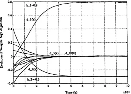
2- 10 Parameter trajectories during adaptation... 45

3- 1 Block processing DFE structure... 52

3-2 Three-input Block DFE... 55

3-3 Block diagram of a (2,1)-DFE... 58

3-4 Decision regions for (2,2)-DFE, h\ = 1.5... 61

3-5 Decision regions for (2,2)-DFE, h\ = 2 /3 ... 62

3-6 Decision boundaries for (2,1)-DFE... 64

3-7 Decision surface for high SNR ( 3 ,1)-DFE, h\ = 1.5, /1 2 = 1... 65

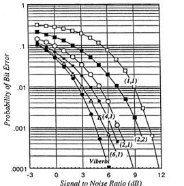
3-9 Probability of error... 67

3-10 Trellis interpretation of a three-input block DFE... 70

3- 11 Decision regions for quaternary signalling... 78

4- 1 Bit error rates with and without error propagation... 96

4-2 Minimum distance to the decision boundary... 100

4-3 Open eye region (starred) for high SNR (2,1)-DFE... 100

4-4 Possible transitions from error state [0,2]... 108

4-5 FSMP regions for (2,2)-DFE... 108

4-6 FSMP diagram for ho = 1, h\ — 0.6, = 0-8... 108

4-7 FSMP regions for the (2,1)-DFE... 109

4-8 Detail of the inner FSMP regions... 110

4-9 Aggregated FSMPs for channel classes A, B, C and D... 112

4- 10 Comparison of stability regions... 114

5- 1 The MAP decision feedback detector... 126

5-2 (2, l)-Detector performance, first order channel... 129

5-3 Detector decision boundary, first order channel... 130

5-4 Conditional probability densities... 131

5-5 Performance comparison on the [1,2,3] channel... 132

5-6 Decision boundaries for SNR=—2dB... 133

5-7 Decision boundaries for SNR—8dB... 134

A-l Binary 4-State Viterbi Trellis... 150

A-2 Merging... 151

G lo s s a r y

L E L i n e a r e q u a l i z e r

D F E D e c i s i o n f e e d b a c k e q u a l i z e r

F F E F e e d f o r w a r d e m u l a t o r

F S M P F i n i t e - s t a t e M a r k o v p r o c e s s

M A P M a x i m u m a p o s t e r i o r i B E R B i t e r r o r r a t e

M L S E M a x i m u m l i k e l i h o o d s e q u e n c e e s t i m a t i o n / e s t i m a t o r

S N R S i g n a l - t o - n o i s e r a t i o

I S I I n t e r s y m b o l i n t e r f e r e n c e

A R M A A u t o - r e g r e s s i v e m o v i n g a v e r a g e

k D i s c r e t e t i m e i n d e x

z ~ l B a c k w a r d s h i f t o p e r a t o r , z ~ l u k = u k - \ m R e a l n u m b e r s

c

IB B i n a r y s y m b o l s e t : { —1 , 4 - 1 } IE B i n a r y e r r o r s e t : { —2 , 0 , 4 - 2 }

~E E x t e n d e d b i n a r y e r r o r s e t : { —2 , —1 , 0 , 1 , 2 } L C h a n n e l o r d e r

F I R ( Z ) F i n i t e i m p u l s e r e s p o n s e ( f i l t e r w i t h L4-1 t a p s )

H R I n f i n i t e i m p u l s e r e s p o n s e

i i d I n d e p e n d e n t a n d i d e n t i c a l l y d i s t r i b u t e d

K T r a n s m i t t e d m e s s a g e l e n g t h

u k C h a n n e l i n p u t s y m b o l a t t i m e k

V k S a m p l e d r e c e i v e d s i g n a l a t t i m e k

n k A d d i t i v e n o i s e s a m p l e a t t i m e k

K i th s a m p l e d c h a n n e l i m p u l s e r e s p o n s e c o e f f ic ie n t H ( z ) z - T r a n s f o r m o f d i s c r e t e - t i m e s e q u e n c e { h k }

u k I n p u t s y m b o l e s t i m a t e a t t i m e k , o r d e c i s i o n d t D F E f e e d b a c k f i l t e r t a p i

{ A , b , c , d } { F , G , H , D }

S i n g l e - i n p u t , s i n g l e - o u t p u t A R M A c h a n n e l r e a l i s a t i o n

B l o c k p r o c e s s i n g c h a n n e l r e a l i s a t i o n

P B l o c k siz e , e q u a l t o d e c i s i o n d e l a y —1 U k , Y k , N k p- v e c t o r s o f s u c c e s s i v e u k , y k , n k r e s p e c t i v e l y

x k C h a n n e l s t a t e a t t i m e k , L - v e c t o r f o r F I R ( L ) c h a n n e l x k C h a n n e l s t a t e e s t i m a t e a t t i m e k

E k S t a t e e s t i m a t i o n e r r o r o r e r r o r s t a t e a t t i m e k e k - j C o m p o n e n t s o f E k, j = L, . . . , 1

Z k U k

D e c i s i o n d e v i c e i n p u t p -v e c t o r , c o m p o n e n t s zkt\ , . . . , z kiP p- v e c t o r e s t i m a t e o f U k

P r ( E ) P r o b a b i l i t y o f e v e n t E

P v ( vk ) P r o b a b i l i t y d e n s i t y o f i i d r a n d o m v a r i a b l e s

P T r a n s i t i o n p r o b a b i l i t y m a t r i x o f f i n i t e s t a t e M a r k o v p r o c e s s Pij (i , j ) e l e m e n t o f t r a n s i t i o n p r o b a b i l i t y m a t r i x

TTfc S t a t e p r o b a b i l i t y d i s t r i b u t i o n v e c t o r o f F S M P a t t i m e k W i j ( k )

y { ( k )

B r a n c h w e i g h t c o n n e c t i n g n o d e i t o n o d e j ( l a y e r d e p e n d e n t ) O u t p u t o f n o d e ( i , j ) a t t i m e k

A N u m b e r o f l a y e r s in f e e d f o r w a r d e m u l a t o r

A ( k ) A g g r e g a t e d s t a t e o f F S M P { E k , — E k ] , v a l u e s A ( i ) M N u m b e r o f a g g r e g a t e d s t a t e s , A t = ^ ( 3 L + 1)

C h a p te r 1

I n tr o d u c tio n

1.1

T h e E qualization P rob lem

1.1.1 L ead In

The equalization problem arises in the area of digital communication. It is desired to transmit a stream of discrete-time digital information through some physical medium, called the channel, to a receiver. Physical channels, having finite band­ width, tend to introduce distortion of the transmitted data which manifests itself in the time domain as a spreading of the energy or duration of the individual data pulses. The continuous received waveform is sampled at the receiver, generating a train of pulses. For practical sampling rates, each received pulse contains contribu­ tions from more than one transmitted pulse. This dispersion of information is known as intersymbol interference (ISI). At high data rates or on highly dispersive channels ISI becomes the major factor hindering the reliable recovery of the transm itted sig­ nals. The part of the receiver which is responsible for the removal or mitigation of the effects of ISI is called an equalizer. The compensation process itself is referred to as equalization.

t r a n s m l t t a r _{1 n o i s e}

est i mat ed symbol s e q u e n c e --- . Input symbol se que nce

s a m p l e r c h a n n e l m o d u l a t o r

t r ansmi t f i l t e r

e q u a l i z e r r e c e i v e

f i l t e r d e m o d u l a t o r

r e c e l v e r

-Fignre 1-1: Communication system model.

followed by decoding at the receiver— although coding does not remove ISI, it in­

troduces redundancy in the transmission so that more errors can be tolerated. The

second is to develop new and better equalizer structures. In achieving transmis­

sion rates that approach the theoretical lim its [1], both these approaches need to be

contemplated. Practical developments, such as very high speed digital signal pro­

cessing chips, mean that more and more numerically intensive processing algorithms

can now be implemented, e.g., trellis-coded modulation schemes [2]. We refer the

reader to [3] for a review of coded modulation techniques.

W hile channel coding (as opposed to source coding) seeks to increase the rate

at which information can be sent w ith a given reliability, equalization corrects the

distortion introduced during transmission and allows still higher data rates. We

mention that the two functions of decoding and equalization can often be combined.

This is true in the case of trellis-coding and V ite rbi decoding [4]. The same may

be true of block-coding and block decision feedback equalization (chapter 3). We

w ill, however, only be concerned w ith the design o f equalizers for uncoded data, the

incorporation of coding being a possible subject for future research.

In the following section we present the basic pulse amplitude modulation system

model underlying the development of the various equalizers which form the basis

for chapters 2-5. This model is a commonly adopted starting point for problems in

channel equalization. We also review conventional equalization strategies which are

c u r s o r ---.

p o s t c u r s o r ISI p r e c u r s o r ISI

Figure 1-2: Sampled channel impulse response.

received noise sequence n ^ si gnal

d e c i s i o n s

d a t a

e f f e c t i v e channel

Figure 1-3: Baseband equivalent model.

1 . 1. 2 D i g i t a l C o m m u n i c a t i o n S y s t e m M o d e l

We restrict the present discussion to pulse amplitude modulation [5] (PAM) over a

linear channel. The system block diagram is given in Fig.1-1. The input symbols

or data {u;t) take values in a discrete set (for binary transmission the symbol set is

{ — 1, + 1 }), and are indexed in time by the subscript k (representing the kth sampling

instant). The data are passed through a transmitter filter and modulated by a carrier

signal before input to the channel (which is often assumed to be linear). Fig.1-2

shows the sampled impulse response of a representative communications channel

and some associated terminology. Random fluctuations in the channel, modelled

as additive noise, also corrupt the signal. The received signal (z in Fig.1-1) is

demodulated (with correct carrier phase and frequency, i.e., coherently), fdtered

and then sampled (with correct timing phase) at the symbol rate to produce the

signal 3/jt, which, for equalization purposes, we will refer to as the received signal. This conversion from continuous to discrete time loses no information as long as

we use a matched filter [3] before the sampler. The equalizer estimates the data

sequence from the received signals and these estimates u^ are called decisions. The

process resulting in y^ can equivalently and more conveniently be represented in the

baseband equivalent form shown in Fig.1-3.

one filter which we may view as the effective channel. The received signal can be expressed as the convolution of the channel impulse response (parametrised by /i,, i = 0 , . . L) and the input symbol sequence, with additive noise rik viz:

( l . i . i )

— ho^k T 'y ^ h{U)c—i T njt,

; = i

in which the channel order L may be infinite. We refer to the coefficient ho as the cursor, which, without loss of generality, we can (and usually do) take to be unity. In writing (1.1.1) in this form, we are assuming implicitly that there is no transmission delay (since yk depends on u^), and, in treating ho as the cursor (which is generally the dominant coefficient), we are assuming that some linear filtering in the receiver has cancelled the precursor ISI. The middle term in the last equation therefore represents the remaining (postcursor) ISI. The vector of the L most recent past channel inputs

is called the state. (We can also define a channel state in the HR case.) This idealized model is a commonly adopted starting point [6] for problems in channel equalization of uncoded pulse amplitude modulated data.

Further assumptions concern the statistics of the input and noise sequences (e.g., correlated or independent) and the type of channel (e.gr., linear or non-linear). In the following chapters we will mostly consider the case in which:

1. The input to the channel is a sequence of independent and identically dis­ tributed (iid) multi-level random variables.

2. The channel is a linear finite impulse response filter.

3. The noise is a sequence of independent zero-mean Gaussian random variables.

The independence of the data teamed with assumption 2 guarantees that the base­ band system, from the point of view of the receiver, can be modelled as a finite-state machine with noisy observations, or a finite-state Markov process [7, 8]. That is, we

can characterise the system in terms of its initial state and the transition probabil­ ities between its various states.

For simplicity of presentation, we will mainly be concerned with binary signalling, although extensions to Af-ary signalling and quadrature amplitude modulation will be covered in chapter 3. There, we will also deal with the equalization of infinite impulse response and non-linear channels. We do not consider how to modify the equalizer structures we develop for coded data.

1.1 .3 E q u a lize r D e s ig n and A n a ly s is

The equalization problem now reduces to the design of a system th at reliably recovers the data {?u} from the received signals {yk}- In practice, the following points need to be considered:

1. Lack of knowledge and time variation of the channel parameters.

2. Computational complexity and decoding delay of the equalizer.

3. The signal-to-noise ratio (SNR).

4. The required bit error rate (BER).

maximum bit rate that can be transmitted. Broadly speaking, the lower the required bit error rate, the higher the complexity/delay of the equalizer.

The bulk of this thesis focuses on non-adaptive aspects of equalizer systems (with the exception of parts of chapters 2 and 3). Although, in practice, the adaptation of an equalizer is of crucial importance to its operation, the importance of under­ standing the underlying mechanisms which cause errors (incorrect decisions) in the tuned (correctly adapted) device cannot be overemphasized. Our main concern is the non-adaptive performance of non-linear equalizers and we give only a brief ac­ count of adaptation in the conventional equalizers which we review in the following sections (the reader is referred to [6] for a comprehensive coverage).

The term non-linear equalizer is understood to mean a system for the recovery of transm itted data whose operation, in the non-adaptive mode, cannot be repre­ sented by a linear filter. The non-adaptive performance of a non-linear equalizer, as measured by its bit error rate (BER), is related to the criterion (subject to practical constraints) used in its design. Some examples of design criteria are: maximum likelihood sequence estimation, minimum bit error rate detection, minimum mean square error and zero-forcing criteria. Two major practical constraints in the real­ isation of an equalizer are the computational complexity and the inherent delay in obtaining data estimates.

In most (but not all) non-linear equalizers, there is some kind of feedback of past decisions. The mechanism for this may be either direct, as in a decision feed­ back equalizer (DEE) [5, 6], or indirect, as in reduced-state sequence estimators (RSSEs) [10, 11, 12]. The presence of a feedback mechanism complicates the per­ formance analysis. The problem of computing the output error probability, Pr(uk / Ufc), usually a relatively straightforward calculation for a linear equalizer or feedfor­ ward equalizer, is made more arduous by the dependence of present outputs on past outputs via feedback (recursion). Nonetheless, we can distinguish two partial solutions to the problem of non-linear equalizer performance analysis:

2. The analysis of errors produced by initial error states and propagated subse­ quently, in the absence of noise.

A complete understanding of error performance requires both of the above analyses. Many authors consider analysis 1 mandatory but 2 is often left out (for examples of 1, see [13, 14]). When there is feedback or use of past decisions, initial errors can produce further errors, enhancing the bit error rate due to noise alone, so that analysis 2 becomes a study of error propagation. One of the themes in our work is a study of error propagation in a generalised decision feedback equalizer called a block decision feedback equalizer [15]. The block DFE (in certain cases) is amenable to analyses of the kind applied to the conventional DFE [16, 17, 18]. The theory of finite-state Markov processs is an invaluable tool for modelling such systems.

1.2

E stab lish ed T echniques

With the intention of setting the scene for the new techniques that we have de­ veloped, we now review three basic equalization strategies in increasing order of complexity and performance. These are the linear equalizer (LE), the decision feed­ back equalizer (DFE) and the maximum likelihood sequence estimator (MLSE) [19]. We also examine the reduced-state sequence estimator (RSSE) [11] which has close ties with the MLSE and the DFE. An understanding of the workings of these sys­ tems will be important in what follows. Certain detailed aspects of MLSEs and RSSEs have been relegated to appendix A.

1.2.1 Linear E q u a liza tio n

del ay el e me nt s a mp l e d r e cei ved s i g n a l s

(k) — 0 -(k) — 0

d ata e s t i m a t e s

Figure 1-4: Adaptive linear transversal equalizer.

channel

feedback filter

Figure 1-5: Non-adaptive decision feedback equalizer.

ZFE is typically less robust than the LMSE and can only be used on eye-open1 ISI channels [20]. A decision device—a hard limiter in the case of binary signals, or vector quantizer for M -ary signalling—can be added at the output of the linear equalizer to improve its noise immunity. This configuration is sometimes called a decision directed equalizer (DDE), although this terminology is more often reserved for the description of equalizer adaptation. Blind adaptation of DDE’s has been studied in [21], and [0] provides a general reference on training sequence adaptation of linear equalizers.

1 .2 .2 D e c is io n F e e d b a c k E q u a liz a tio n

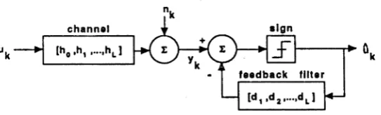
For more severe channel distortion (e.y., non-minimum phase channels whose inverse is unstable) a decision feedback equalizer (Fig. 1-5) may be required. The DFE is a non-linear equalizer with a linear feedforward filter designed to handle precursor

IST, and linear feedback filter and non-linear decision device handling postcursor ISI and noise. For argument's sake, we assume the feedforward part is lumped with the channel response and consider only the operation of the feedback part (treating the dominant impulse response parameter ho as the cursor). Ideally the DFE adapts or tunes its feedback taps rf, to cancel the intersymbol interference (d, = /it, uk~i = Uk-i, i = 1 ,.. .,L ) and passes the ISI-free signal (hoUk + nk) to a quantizer (sheer) which makes a decision on the transmitted signal. In symbols this reads

L L

ük = sgn(/i0ujt + hiuk-i ~ X ] d'Uk-i + n k). (1.2.1)

t = i t = i

v . ___ ^

Vk

The decision feedback equalizer does not utilise the energy contribution from the intersymbol interference in decoding each symbol, it merely tries to cancel it. If the DFE makes an initial incorrect decision uk ^ uk (be it due to noise, incorrect initialization or mistiming) it may fail to cancel the ISI and this occasionally leads to bursts of errors. The phenomenon of an initial error causing subsequent errors is known as error propagation. A more detailed description of the operation of the decision feedback equalizer, covering training sequence adaptation, is set out in [22]. Error propagation in DFEs has been analysed in [23, 24] and blind adaptation in [25].

1 .2 .3 M a x im u m L ik e lih o o d S e q u e n c e E stim a tio n

techniques is given in section 3.4.3.

Using the notation introduced in section 1.1.2, the MLSE operates on finite im­ pulse response channels and determines the length K state sequence {x*.} (or equiv­ alently the input sequence {u*.}) which maximises the conditional probability density P( {2/A:}I{ } ) - A closely related problem, that of maximum a posteriori (MAP) es­ timation, seeks to maximise the a posteriori probability Pr({uk}\{yk})- The two criteria are equivalent when the input sequence is iid and equiprobable [26, 15] and can be interpreted as finding the input sequence which best represents the measurement sequence in a mean square sense. The MAP criterion minimises the probability of incorrectly decoding the whole state sequence. In chapters 3 and 5, we consider non-linear equalizers based on fixed-delay MAP criteria incorporating decision feedback.

For binary inputs to a finite impulse response channel of order L there are 2L possible states (since each component is binary and the state consists of L of these). The MLSE searches over all admissible state sequences and selects the one which minimises a sum-of-squares cost function—arising from the assumption of white Gaussian noise. The delay involved in this brute force computation would be unac­ ceptable for long channels and many authors have considered various related criteria which result in simpler (suboptimal) non-linear detectors [27, 30, 31]. However, the landmark work on the MLSE problem was achieved by Forney [19] with an ap­ plication of the Viterbi algorithm (VA) [32]—a forward-time version of dynamic programming [33]. This recursive solution of the optimization problem, Viterbi de­ coding, makes the MLSE computationally practicable. However, since its complexity grows exponentially with the channel length, the MLSE can only be used on chan­ nels having a short impulse response. Appendix A.l contains a summary of the Viterbi algorithm.

1 .2 .4 R e v ie w o f O th e r T ech n iq u es

[12, 34, 35, 36, 37, 38, 39]. These composite systems try to take advantage of the simplicity of the LE and/or DFE to preprocess and remove a portion of the inter- symbol interference from the received signal, thus presenting an effectively shorter channel and reducing the complexity of the Viterbi decoder required for the remain­ ing task. Although these hybrid equalizers can work well, their success is limited in general by the performance of the LE or DFE they incorporate.

Since the introduction of the Viterbi decoder, an equalizer with performance akin to a MLSE, but needing substantially less computation was the object of intensive re­ search. By the mid 1980's, systematic attem pts were being made at developing such equalizers, or moreover classes of equalizers, with the attributes of relative simplic­ ity and performance ranging between the extremes of the DFE and MLSE. We now mention some of these. One technique is based on reduced complexity Viterbi de­ coding teamed with internal decision feedback. This was introduced independently in [10], under the name delayed decision feedback sequence estimation (DFSE) and by [11], under the name reduced-state sequence estimation (RSSE), who built upon the preceding work of [10]. Another technique, called the A/-algorithm, simply trun­ cates the search used in the Viterbi decoder. A large part of our work relates to the development and evaluation of a device (the block decision feedback equalizer) which also satisfies these requirements. We defer its discussion until chapter 3. A description of delayed decision feedback sequence estimation and reduced-state se­ quence estimation is available in appendix A.2. Both schemes reduce the dimension of the Viterbi trellis in a natural, structured way, retaining the essential features of the Viterbi decoder. In [10] the channel may be recursive (HR), whereas in [11] it is assumed to have finite impulse response.

1.3

O u tlin e o f T h esis

1 .3 .1 S u m m a r y and C o n tr ib u tio n s

We now proceed with a chapter-by-chapter description of the thesis, pointing out the major contributions.

emulates a decision feedback equalizer. The so-called feedforward emulator (FFE) arises through a recursive unwrapping of the DFE, followed by truncation (cutting off the feedback path). This unwrapping procedure is analogous to a Markov ex­ pansion [41] of a linear (finite dimensional) HR system. The DFE with feedback is replaced by a multilayer feedforward processor and generates data estimates with delay corresponding to the number of layers.

In section 2.3 we obtain an upper bound on the noiseless error probability (due to non-zero initial conditions) by generalising the existing theory for the DFE [23]. The method entails modelling exactly the feedforward emulator as a DFE th at has been initialized at each time instant in a non-standard error state. Then, modelling the DFE by a finite-state Markov process writh a large number of states, aggregation is performed by choosing a worst case channel (specialised to the FFE case) and an exponential upper bound for the FF E ’s error probability is obtained in terms of the number of layers. The bound is realized by worst case channels but seems to be conservative for most practical (decaying) channels. The importance of this work is that it brings hard analysis to bear on the non-adaptive performance of a neural network-like structure which may have more general application. The norm in most w'ork on neural networks is the recognition that a multi-layer perceptron neural network can perform a certain task adequately (i.e., non-linear mapping), but the justification often rests solely on the experimental or simulated performance.

The structure of the feedforward emulator is constrained by the requirement that it should act as an equalizer. This manifests itself in the number of nodes per layer, the connectivity between nodes and the interdependence of the weights. It turns out th at, for a FFE with A layers, only A - 1 of the ^A(A + 1) weights are independent (as the matrix of weights is Toeplitz). Thus only A — 1 quantities need be adapted during training (or tracking). Using back propagation ideas [40, 42], recursive gradient descent algorithms have been developed and tested for a FFE consisting of (1) sign nodes and (2) sigmoid nodes.

se-quence estimator). In some respects our contribution, the block decision feed­ back equalizer, is complementary to reduced-state sequence estimation (see appendix A.2). Whereas the latter approach is based on reducing the complexity of an MLSE using the idea of a subset state, our approach seeks to improve the performance of the DFE by generalizing it to the vector case. In a manner of speaking, the RSSE is a top-down approach (the MLSE being perceived as the “top”) and the block DFE a bottom-up approach. Precursors to the block DFE were studied in [13, 14, 43, 44], although the block DFE was developed independently.

The block DFE (Fig.3-1) is a natural generalization of the conventional DFE. It is based on a block processing [45, 46, 47] channel model connected in feedback with a vector quantizer [15] operating under a maximum a posteriori criterion. The block DFE, or (p, </)-DFE, is indexed by two parameters: the block length p and the number of decisions q produced at each (block) iteration. The block length is independent of the channel length. It can be made to replicate the DFE when p = q = 1, the MLSE in the limit as p = q —* oo and the maximum a posteriori symbol- by-symbol detector [30, 31] when q = 1 , p —* oo. The best performance (for fixed p) is achieved in the latter mode with q = 1, p large, where the (p, 1)-DFE functions as a minimum bit error rate detector. We investigate these connections in section 3.3.5

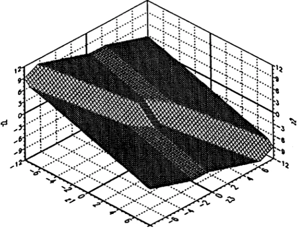
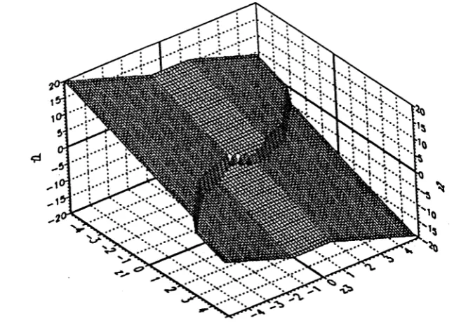
Exam-pies of two and three-dimensional block DFE realisations and their vector quantizers are also given. Some other interesting examples of two-dimensional decision devices (and their corresponding decision boundaries) which optimize various criteria (in­ cluding maximum likelihood decision boundaries for non-linear FIR channels) may be found in [50, 51, 52]. The block DFE can operate on linear infinite impulse re­ sponse (ARMA) channels and also non-linear channels having a finite-dimensional state space realization. Generalization to M-ary signalling, coloured noise and adap­ tation of block DFE parameters are considered in section 3.5.

Block DFE performance analysis forms the substance of chapter 4. All analyses of the block decision feedback equalizer so far concentrate on the 2-input (p = 2) case. The analysis is complicated by the non-linearity of the decision device and its dependence on the channel parameters. The decision boundary is the curve separating the different decision regions in the decision device. This boundary is curved for a (2,1)-DFE but becomes piecewise linear for high signal-to-noise ratios. (The (2,2)-DFE decision boundary is always piecewise linear.) Simple geometrical considerations yield an explicit formulae for the decision boundary, and are the starting point of performance/stability analyses of the (2,1)-DFE and (2,2)-DFE.

We give a representative example calculation in section 4.3 of the (2,l)-D FE ’s primary error probability on a first order channel, i.e., the bit error rate assuming that there have been no past decision errors. In section 4.4 we derive eye conditions for finite error recovery of the (2,1)-DFE on an arbitrary second order channel.

4.5. Example calculations of the mean and variance of error recovery times are also presented. These preliminary results show that the block decision feedback equal­ izer is stable on a broader class of channels and is therefore more robust than the decision feedback equalizer.

As is common in decision feedback equalization, the block D FE’s criterion uses the assumption of correct block ISI cancellation (or channel state estimation) in the design phase. In chapter 5 we consider a different criterion, related to fixed- delay, symbol-by-symbol MAP detection, which does not rely on this assumption and subsequently generalises the block DFE, although it only operates on finite impulse response channels. The resulting non-linear equalizer is called a maximum a posteriori decision feedback detector [54], and incorporates knowledge of certain error probabilities, giving improved performance. The design of the detector is covered in chapter 5 in which we also present a recursive procedure for its realization (this is necessary since the decision criterion cannot be expressed in closed form). We provide simulated performance comparisons for the new detector on first and second order channels, showing the improvement in bit error rate over the block DFE, and give examples of the decision regions that are thus formed.

C h ap ter 2

F eed fo rw a rd E m u la tio n o f th e

D e c is io n F eed b a ck E q u a lizer

2.1

In tro d u ctio n and M otivation

The decision feedback equalizer is a simple but effective non-linear equalizer that has enjoyed widespread application in digital communication systems [6]. Its op­ eration has been studied by various authors [16, 17, 36, 55] and is reasonably well understood. The simplest realisation of a DFE is the non-linear recursive structure shown in Fig.1-5. On the other hand, the multi-layer perceptron (MLP) neural net­ work [40], which also has been applied to the equalization problem in [52, 56], is a relatively poorly understood system. In this chapter, we consider an intermediate structure for equalization, the feedforward emulator (FFE) [57, 58, 59], which derives from the DFE and is closely related to the feedforward neural network, and which may be analysed in much the same way as the DFE.

enhance-ment of standard MLP neural network equalizer techniques because there is a direct link between the weights and the parameters characterising the channel.

The chapter is organised as follows. In section 2.2, we briefly review the non- adaptive decision feedback equalizer and detail an unwrapping procedure followed by truncation that results in a recursive multilayer processor with hard limiting nodes. We obtain the feedforward emulator by disconnecting the feedback of decisions made in the distant past. We give some low order illustrations and show how the structure generalises to an arbitrary number of layers.

In section 2.3 we re-introduce the finite state Markov process description of the tuned noiseless decision feedback equalizer found in [17]. We extend the model to embrace both the DFE and the feedforward emulator by enlarging the state space. In section 2.3.2 we introduce the idea of a worst case channel, i.e., a FIR channel guaranteeing the worst bit error rate performance for any channel of the same order. We subsequently apply FSMP theory to upper bound the noiseless error probability of the DFE (in section 2.3.3) and then the FFE (in section 2.3.4), obtaining a bound in terms of the number of layers for the latter. We present numerical examples for the non-adaptive feedforward emulator in section 2.4 and also examine conditions on the channel under which the representation is exact (in the sense of producing the same sequence of outputs in the absence of noise).

2.2

U n w rap p ing th e D ecisio n Feedback E qualizer

Conventional multi-layer perceptron neural networks, which can be configured to act as non-linear equalizers [52], are highly interconnected non-linear systems whose analysis is typically very difficult. In contrast to this, we derive a new non-linear feed­ forward processor designed to emulate the well-studied decision feedback equalizer. The new structure is more amenable to analysis and it is possible to obtain bounds on its performance in the absence of noise—which we assume for simplicity only. We therefore consider a non-adaptive binary decision feedback equalizer operating on a finite impulse response channel corrupted by additive zero-mean white Gaussian noise nk. At the output of the channel, the sampled received signal is

L

Uk — ^ ^ hjU-k—i T H-ky (2.2.1)

t = 0

where {/i,} are the impulse response coefficients and {uk} is a sequence of equiproba- ble iidbinary inputs which we cannot measure directly. The DFE (Fig. 1-5) generates an estimate of the input signal, based on its own past decisions, given by1

L

uk = sgn(yk - ^dj(Ar)wjt-j) = f £( yk\ ujt-i, • • •, Ufc-Z,)* (2.2.2) j=i

The feedback tap gains dj(k) are adapted to cancel the intersymbol interference in­ troduced by the channel. Initially, we will be presenting an analysis of the non- adaptive system in which the dj(k) = d3 are constant. We assume, with no loss of generality, that /?0 = 1.

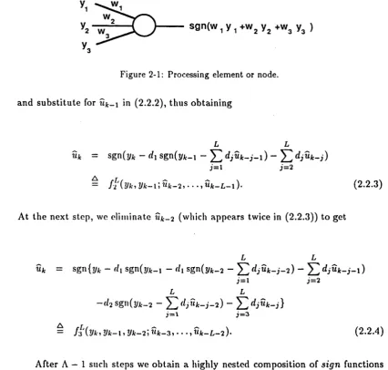
We develop a self-similar recursive representation of (2.2.2) by “unwrapping” the DFE, and, in so doing, introducing a delay in the computation of the decisions. As we mentioned in chapter 1, this procedure is analogous to the Markov expansion of an ARMA filter. At the first step we write

L

Uk- l = Sgn(t/jfc_i - ^djUAr-j-l),

sgn(w

1

y

1

+w

2

y

2

+w

3

y

3

)

Figure 2-1: Processing element or node,

and substitute for uk- \ in (2.2.2), thus obtaining

L L

uk = sgn(yk - sgn(yjt_i “ 1) - ^ 2 djUk- j )

j= 1 J = 2

= f H Vi*, V k - (2.2.3)

At the next step, we eliminate uk - 2 (which appears twice in (2.2.3)) to get

L L

w* = sgn{yk - (lI sgn(?/jt_i - sgn{yk_2 ~ ^ r f j W i t - i -2) - Y l df i k- i - \ )

J=l J=2

L L

- r / 2sgn(i/jt_ 2 - ~ Y l dP lk- i )

J=V j=3

— y*3 ( 2/A*» !//►—1» 2/A:—2» Wfc—3, . . ., Wfc_£,_2)- (2.2.4)

After A — 1 such steps we obtain a highly nested composition of sign functions whose functional form can be written as

Wit = /a ( 2/it> 2 /it- 1, • • . , » J t - A + r , M f c - A f • W f c - L - A + l ) . ( 2 . 2 . 5 )

There are in fact A degrees of nesting in this expression and we can interpret these as the layers in a recursive multilayer processor whose external inputs are the

{j/fc-A+i, . . . , j/it}, whose feedback inputs are the {ujt-Ai • • •> w j t - A - L + i }> a n d whose output is uk . The processing elements, or nodes, compute the sign of the weighted sum of their inputs. Fig.2-1 depicts a typical node.

Figure 2-2: Three-layer feedforward processor.

This is equivalent to the effect of earlier decisions in a DFE ceasing to influence later decisions, given a large enough time delay between the two. We give substance to this notion in the following sections.

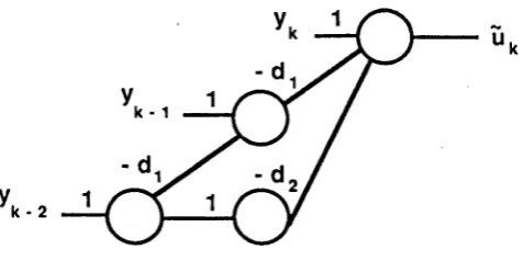
Supposing, then, that we can ignore decisions made in the distant past, we disconnect the feedback implied in (2.2.5) by setting the arguments involving past decisions to zero, obtaining

II k — f \ (l/ki Vk — 1 ? • • • > J/A: —A + l i 0» • • • t 0)* (2.2.6)

If our intuition is correct, then with high probability and given a large number of layers (A large) we would have uk = uk. It is instructive to visualise (2.2.6) as a multilayer feedforward processor with sign nodes. We illustrate in Fig.2-2 the corresponding system in the A = 3 case first (setting iik-j = 0, j > 3 in (2.2.4)).

Before proceeding with the general case embodied by (2.2.6), we make a short digression to examine the noiseless feedforward version of (2.2.4) with A = 3, which may be expressed as

Uk _{f'3 {Vki Vk —} 1 y Vk—2» 0» • • • » 0) |n*=nfc_i =rifc_2=0

L L

Sgn{?/jk + hiuk-i - d 2 sgn(uk- 2 + JZ /l«'uJt-.-2)

«=1 1=1

L L

- d \ sgn(Mjfe__i + h{Uk-i-\ - d x sgn(?u-_2 + ^

/i,wjt-.-2))}-i = /i,wjt-.-2))}-i » = 1

Figure 2-3: Noiseless MLP realisation.

in practice, the input sequence {u*} and the channel parameters are unknown, but the purpose of Fig.2-3 is to show how Fig.2-2 can be captured in a standard MLP neural network framework.

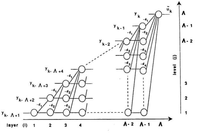
Returning to (he general A-layer structure described before in (2.2.6), it is fairly easy to generalise the low order cases to arrive at the diagram in Fig.2-4. This feedforward parallel processing structure, which implements (2.2.6), will be referred to in the sequel as a A-layer FFE. We have drawn Fig.2-4 to accentuate its Toeplitz structure—the weight of the branch connecting node i in layer k to node i 4- j in layer k -f- 1 is —<lj, independent of i. We alert the reader to the following important differences between Fig.2-4 and a standard MLP neural network.

• Eacli diagonal node has one external input, this being a noisy channel output.

• All horizontal connections have fixed weight one.

• There are only A - 1 distinct weights.

A

K- A +4

k- A +3

k- A +2

k- A +1

A- 2 A- 1 layer (I) 1

Figure 2-4: Feedforward em ula tor for the D F E .

Each node c o m p u tes the sign of the weighted su m o f its inputs. T h e weights are marked on the branches and horizontal connectio ns have weight 1.

2.3

A n a ly sis o f N o ise le ss Error P ro b a b ility

2 .3. 1 F i n i t e S t a t e M a r k o v P r o c e s s D e s c r i p t i o n

We can accurately model the stochastic dynamics of the DFE using the theory of finite state Markov processes [8] as long as the input sequence to the channel is independent. Referring to (2.2.1) and (2.2.2), the input is uk and we choose

as the state vector. There are AL states in total if all elements are binary. Since the DFE is assumed to be tuned (in the sense that dj = /ij, j £ (1 , . . . , £ } ) , we can reduce the number of states to 3^ by defining an error state

Ek = [ ' k - L... n - i l ' (2.3.1)

(2.2.2) (with h0 = 1) can be re-expressed as L

uk = sgn(uk + ^ 2 hiek-i + n*). (2.3.2) » = i

In order to simplify the analysis, as is standard in the analysis of error propagation of DFEs [16, 23], we consider only the noise-free case (n k = 0 Vk) so that the unique absorbing state of the FSMP is E k = 0 (the zero vector). To see this, note that the error vector or state satisfies the simple recursion

E k + i

0 1 0 ••• 0 0

0 0 1 ••• 0 0

E k +

0 0 0 ••• 1 0

0 0 0 ••• 0 uk - sgn(ujt + h'Ek)

(2.3.3)

where h = [h\ , . . . , hi]1. If E k — 0 then for all inputs we have sgn(uk + h!Ek) = uk and the DFE remains in the zero-error state regardless of the input. However, from an E k state having a non-zero entry, there is a non-zero probability of reaching the absorbing state in M steps for any M > L (since a sequence of L correct decisions will cause transition to the absorbing state). Also, the probability of ultimately reaching the absorbing state is 1 [16]. When noise is present, only a noise-induced decision error can cause a transition from the zero-error state.

Returning to the recursive representation of the DFE described in the last sec­ tion, we see that the output, in the absence of noise, can be viewed as depending on the sequence of inputs m^ _a+i , . . . , uk and the initial state Xjt-A+i (or E k-a+i )• For convenience, we introduce the notation (with reference to (2.2.5))

/a (iJki • • • i Vk— A + l ! Mfc—a i • • • i Uf c _ A —L —1 ) I n * = •• • = »! * _

= 9 A ( llk, ■ • . , M j f c - A - L - i ; W j f c - A > - • « i f e - A - L - l ) * (2.3.4)

With this in mind, we define an extended state X k (Ek in the tuned case) having the same form as Xk but in which the decisions which appear in the initial state may take the additional value zero. Each element Ek of the extended error state Ek takes values in ZE7 = {0, ±1, ±2}, so there are a total of Ek states comprising the set IEL. Of course, a DFE with an initial state in 1EL reverts to a DFE with state in IE1 after L time units because the binary decisions that are fed back will displace the initial conditions. The concept of an extended state, together with the error probability bound, will allow us to gauge the effect of omitting the recursive part (i.e., old decisions) in the representation for the DFE (2.2.5), thus obtaining a feedforward structure generated by

Uk 9 • • • i Uk — \ ± \ , V. k — i U k—A — L — — A • — 0 , . . . , T Z j f e _ A — L — 1 0 ) »

(2.3.5) (or by (2.2.6) in the noisy case) where Uk is binary, but, by the notation u^-A +i-j := 0, we mean that any feedback paths in the recursive processor (2.3.4) have been deleted. Note that the same Uk as (2.3.5) would be generated by a standard DFE, started in an abnormal initial state E k - \ + \ with fictitious past decisions Uk~\ =

0 ,. . . , U k - A - L - i = 0 and fed with the sequence of inputs U k -a+i , . . • , Uk. Thus, the

feedforward structure in (2.3.5) is effectively a “sliding-window” version of the DFE which resets its initial conditions at each time instant. We shall have more to say about this in section 2.3.4.

2 .3 .2 W o rst C ase C h a n n els

Extending the development found in [23 ], we now determine a class of channels on which the DFE has the worst possible performance (in terms of error propagation) from an arbitrary initial condition in the extended error state space 1EL. This will allow us to bound the DFE’s noise-free performance, and subsequently the feedforward emulator’s performance, on an arbitrary FIR channel.

Any channel

satisfying

jn in \hTEk\ > 1 (2.3.6)

E r f o

has the property that P r ( u k / uk) = \ for any non-zero extended error state E k.

This follows since the inputs are equiprobable and therefore uk has a probability

of I of having the same sign as h'Ek (recall that uk = sgn(ujt + h'Ek)). Channels

satisfying (2.3.6) will be termed “worst case” channels. We claim that the expected

error recovery time2 is maximised for such channels, which form a subset of the

worst case class in [16] since we are allowing Ek to have the additional values ±1.

Any channel (with /i0 = 1) whose parameters belong to the set

L j -1

{h

e

n L

I ft, > 1} P |

{h

e

ntL \ hj

> 1 + 2

Y

*}.

j =2 k=l

will fall into the worst case category. This is because the hj have been spaced so

far apart that no linear combination with coefficients in the set { 0 ,± 1 ,± 2 } has

magnitude less than 1. (The same is true of any channel that can be obtained from

this set by changes of sign and/or permutation of parameters.)

As an illustration, consider the L

=

h\

=

min I[1.2,3.5] E k\ = 3.5 - 2 x 1 . 2 = 1.1 > 1, E k* o

demonstrating that [1,1.2,3.5] is a worst case channel. That is, no second order

FIR channel may have an expected recovery time which exceeds that of the above

channel.

2 .3 .3 B o u n d for th e D e c is io n F eed b ack E q u a lizer

In what follows we may assume the DFE is operating on a noiseless worst case

channel so as to obtain a tight performance bound. The order of the FSMP model

can further be reduced by aggregating states, provided that states to be aggregated

have identical transition probabilities [60]. Here, we are able to impose a structured

aggregation of the 5L — 1 non-zero extended states E k while retaining the Markov

property between the aggregated states. We choose to aggregate the E k states

Figure 2-5: Aggregated FSMP for a worst case FIR(L) channel.

according to the following rule [18].

D efinition 2.3.1 (A ggregation R ule) The extended error state Ek (it time k, defined by (2.3.1) with components in IE, is in aggregated state Ck = q if there exists a binary input sequence {wj}j*2_l such that the absorbing state Ek+q = 0 is reached in q steps (while it cannot be reached in fewer).

From the shift register property (2.3.3) applied to Ek (by allowing «jt = 0), it is clear that at most /, successive correct decisions are needed to force an arbitrary non-zero Ek state to the absorbing state. Hence there are L + 1 aggregated states ejt in the new FSMP. From a given state €k = q (q / 0) there is a probability of | (for equiprobable inputs) of transiting either to state cjt+i = q — 1 (with a correct decision) or to state (k+i = L (with an incorrect decision) at the next time instant (see Fig.2-5). Subsequently, the transition probability matrix can be partitioned as

P = (Po) Q 0

l

r' 1

e /7j>(L+l)x(L+l) _(2.3.7)

where

Pij = Pr(€k+\ = L + l - i \ € k = L + l - j ) and

Q =

1

2

e

mLxL

r' = [ 0 , . . . , 0,1/2] E m L.

(2.3.8)

L + 1 — i, or

7Tk,i = Pr(ek = L + 1 - *), i = 1 , . . . , I + 1, Then this state distribution vector evolves according to

TTfc+l = P x i fc. (2.3.9)

Now suppose the initial extended error state £o € ZE^ induces the distribution 7To at time k = 0. We can compute the probability of the system failing to reach the absorbing state €fc+i at time k + 1, while operating on a worst case channel, as

L

Pk(iro) = Pr(ek+\ # 0 I 7T0) = ^ P r ( c j t +i = i | tt0). (2.3.10) t = i

In other words, pk(^o) is the sum of the first L components of the vector 7r*. If we partition Xk conformably with (2.3.7) as

7Tfc = ’ * k L p

and make repeated use of (2.3.9), we have

Pa(tto) = [ 1 • • • 1 OJtta; = [ 1 - • l J Qk7T0,

L + i L

in which 7fo is the initial distribution across non-zero aggregated error states ek. Applying the power method to the matrix Q, we obtain the upper bound stated in the following theorem (this result is a mild generalisation of the analogous result in [23] concerning the DFE).

T heorem 2.3.1 (N oiseless Error Bound - D FE ) Consider' the tuned DFE with output given by (2.3.2) with nk = 0, operating on a noiseless worst case FIR channel of order L, and initially in non-zero extended error state Eq E IEL at time 0. If Eq induces the aggregated state distribution 7To, the probability of not reaching the absorbing state ek = 0 at time k is given by

L 2 3 4 5 6

Ai 0.8090 0.9196 0.9638 0.9830 0.9918

Table 2.1: Dominant eigenvalue of Q.

where oq = w[WqG (0.1 ],

Ai = max \ i (Q) G (0,1),

1 < t < L

is the unique dominant eigenvalue of Q defined in (2.3.8), and w\ = w \/\w i \ G 2RL where W\ is the eigenvector of Q corresponding to Ai, given by

L- 1 L —2

w \ =

[1, XI

XI Z*7» •••»** + A*2»

3 =1 3- 1

uu7/i /* = (2Ai) 1.

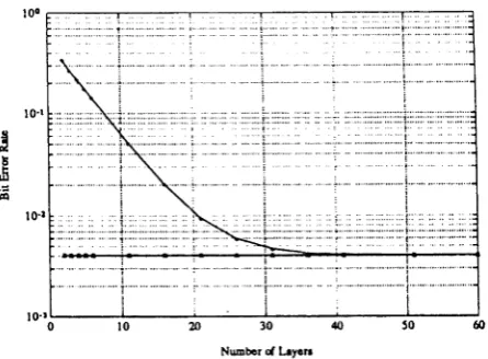
Since the calculations assumed a worst case channel, the above bound indicates the highest degree, on average, to which an initial error can influence subsequent decisions by error propagation alone on any noiseless channel. The bound may be conservative in that Ai ss 1 for worst case channels. We list Ai for various channel lengths (L) in Table 2.1. For practical channels (e.g., with decaying impulse responses) the exponential form of the bound is still valid (with correspondingly smaller Ai), but in general it is not possible to aggregate the FSMP model to obtain the Zth order description used above, so the full order bL non-aggregated FSMP would need to be used.

2 .3 .4 B o u n d for th e F eedforw ard E m u la to r