Local RBF Approximation for Scattered Data Fitting
with Bivariate Splines
Oleg Davydov, Alessandra Sestini and Rossana Morandi
Abstract
In this paper we continue our earlier research [4] aimed at developing efficient meth-ods of local approximation suitable for the first stage of a spline based two-stage scattered data fitting algorithm. As an improvement to the pure polynomial local approximation method used in [5], a hybrid polynomial/radial basis scheme was considered in [4], where the local knot locations for the RBF terms were selected using a greedy knot insertion algorithm. In this paper standard radial local ap-proximations based on interpolation or least squares are considered and a faster procedure is used for knot selection, significantly reducing the computational cost of the method. Error analysis of the method and numerical results illustrating its performance are given.
1
Introduction
LetX⊂Ω, be a set of scattered distinct sites and {(x, fx) : x∈X, fx∈R} the set of
data points to be approximated, Ω⊂Rd. The idea of the two-stage method [16] is to compute in the first stage a large number of local approximations to the data and use them in the second stage as a source of information (e.g., function values and gradients at vertices of a triangulation) for building aglobal spline approximation of the full data set using a localized quasi-interpolation type operator. This helps to avoid solving large linear systems and large scale optimization problems arising if the interpolating, smoothing or minimal energy spline is directly computed from the data. For a long time it has been believed that two-stage methods cannot produce approximations of the same quality as the above mentioned global methods.
Recently, a promising two-stage bivariate spline algorithm has been developed and tested in [5, 9]. Convincing numerical evidence has been provided that the new method is efficient, robust and avoids the drawbacks usually associated with the two-stage methods. One of the goals of [4] and this paper is to improve the performance of this method at the first stage by achieving the approximation quality of the radial basis function (RBF) methods [2], in the same time also avoiding their well known computational difficulties, by applying them only to small subsets of the data.
[3]. In [4] and here we consider local approximation schemes defining non-polynomial approximations which are later converted into polynomials and then extended to a spline by the same method as in [5]. In [4] we have provided numerical evidence that better accuracy of the approximation may be achieved if local polynomials are augmented by linear combinations of radial basis functions, so defininghybrid approximations which are still computed by discrete least squares. The knot set used for each local hybrid approximation is chosen using an adaptive greedy algorithm based on successive knot insertion and estimates from [3].
In this paper we consider the standard radial approximations in the local stage that are computed by interpolation or by the least-squares method, with the local knots selected using a thinning algorithm similar to that suggested in [7] in the context of multiresolution. (Note that our motivation for thinning is entirely based on the compu-tational considerations since the condition numbers of the matrices arising in the RBF method depend on the so calledseparation distance of the knots.)
The paper is organized as follows. In Section 2 we introduce the local approximation scheme. In Section 3 we provide an error analysis of this version of the two-stage method based on available estimates for the RBF interpolants. Sections 4 and 5 are devoted to extensive numerical tests with two goals: to verify the approximation order of the method, and to compare the performance of this new method with the method of [4] for some real world data sets.
2
Local RBF Approximation
At the first stage of a two-stage method, the local approximations are needed for each cell T of a partition of Ω associated with the spline method used. (Such a cell is usually ad-dimensional simplex or cube.) The task of the first stage is to find a good approximation of the underlying function onT. To this end, the data from some domain
ω, where T ⊂ ω ⊂ Ω, are used. As in [4, 5, 9], we select the domain ω initially as a ball with center at the barycenter of T and of radius equal to the diameter of T. If the number of data points located in this ball is smaller than a user specified number
Mmin, then the radius of the ballω is enlarged until this number is achieved. Another
user specified parameter,Mmax, controls the maximal number of points to be used, and
a uniform type thinning is employed, if needed. Thus, this data selection procedure delivers a set of data sitesXω={x1, . . . ,xNω} ⊂X∩ω. where
Nω ≤Mmax. (1)
The local RBF approximation has the following form
ℓω(·) = m
X
j=1
ajpj(·) + nω
X
j=1
bjφω(k · −yjk2), (2)
where the set of knots Yω = {yj : j = 1, . . . , nω} is a subset of Xω, {p1, . . . , pm},
m= d+dq
q≥0, andφω :R≥0→Ris aradial basis function, i.e., a positive definite function or a
conditionally positive definite function of orders≤q+ 1 on Rd [2], adjusted to the size ofω by scaling. Thus, we take
φω(r) =φ
r
δdω
, r≥0, (3)
whereφis a fixed radial basis function,dω is the diameter ofω, andδ is a user specified
parameter.
In this paper we consider only positive definite radial basis functions or conditionally positive definite radial basis functions of order 1. Therefore, it is sufficient to take
q= 0.
The functionℓω of the form (2) is selected by using interpolation on the coarse set
Yω, i.e. requiring
ℓω(yj) =fyj, j= 1, . . . , nω, (4)
with additionalorthogonality condition
nω
X
j=1
bj = 0. (5)
The existence and uniqueness of such a function is guaranteed for anyYω (see e.g. [2]).
In particular, the matrix of the corresponding linear system,
eT AYω
0 e
,
wheree:= (1, . . . ,1),
AYω :=
φω(ky1−y1k2) . . . φω(ky1−ynωk2)
..
. ...
φω(kynω −y1k2) . . . φω(kynω−ynωk2)
,
is nonsingular as soon as all knotsy1, . . . ,ynω are distinct.
Since the linear system arising in this interpolation problem is of the size nω+ 1≤
Mmax + 1, its solution can be easily computed if Mmax is not large, and if the matrix
AYω is well conditioned.
To complete the description of the method we now explain how we chooseYω. It is
known that the condition number ofAYω can be bounded in terms of the reciprocal of
theseparation distance
s(Yω) =
1
21≤i<jmin≤nωkyi−yjk2.
Therefore, we chooseYω such that
whereSis again a user specified number. To guarantee (6), the thinning algorithm from [7] is adapted.
As an alternative to interpolation, the discrete least squares approach [10, 12] can also be considered, i.e. ℓω of the form (2) can be selected via the minimization of the
least-squares error (the ℓ2-norm of the residual onXω),
XNω
i=1
(fi−ℓω(xi))2
1/2
, (7)
using the orthogonality condition (5) as a linear equality constraint. The existence and uniqueness of the least squares approximation follows from the theory of constrained least squares, see [1].
Regardless whether we use interpolation or least squares, and besides the choice of the radial basis function φ, the scheme depends on the following parameters that are supposed to be specified by the user globally, i.e., the same values are used for all local approximations:
Mmin, Mmax, δ, S. (8)
In real world applications these parameters have to be adjusted to a particular type of data by some calibration procedure. The local error estimates discussed in the next section can also be useful for this.
3
Error Bounds
To facilitate a correct comparison to the approximation results for global methods, we mention that the approximation order of a two-stage method is the minimum of the order of the spline operator and that of the local scheme [16]. More precisely, let us assume for simplicity that the subdomains where local approximations are needed are thecells T of auniform partition △of Ω associated with the spline space, which is the case for the splines used in [5]. Then the approximation error of the two-stage scheme in the uniform norm for a sufficiently smooth function can be estimated by
C1hp+1 + C2max{eT : T ∈ △}, (9)
whereh is the diameter of the cells,p+ 1 is the approximation order of the spline quasi-interpolation operator, eT is the error of local approximation, and C1, C2 are some
positive constants.
To assess the approximation error of the first stage of the two-stage method we invoke some results from the approximation theory of radial basis functions on bounded domains.
Letℓω(f) be the sum (2) determined by the conditions (4) and (5) withfyj =f(yj),
j= 1, . . . , nω, for a functionf :Rd→R. We assume thatf is smooth enough to belong
to thenative space Fφω associated with the radial basis functionφω,
where
|f|φω :=
Z
Rd
|fˆ(x)|2 ˆ Φω(x)
dx 1/2
, Φω(·) :=φω(k · k2),
and ˆf denotes the generalized Fourier transform.
Well known error bounds for the interpolation with radial basis functions (see, e.g. [2, 11, 13, 17]) lead in the caseq= 0 to the estimate
|f(x)−ℓω(f,x)| ≤2
q
E0(Φω)C(Bh(x,Yω))|f|φω, x∈R
d, (10)
whereh(x,Yω) is the distance between x andYω,
h(x,Yω) := inf
y∈Yωk
x−yk2,
E0(Φω)C(Bh(x,Yω)) is the error of the best constant approximation of Φω,
E0(Φω)C(Bh(x,Yω))= inf p∈Πd
0
kf−pkC(Bh(x,Yω)),
andBr denotes the ball inRd with center 0 and radiusr.
Assuming that φ is monotone (which is true for all available radial basis functions at least in a neighborhood of zero) and considering thefill distance of Yω with respect
to T,
h(T,Yω) = sup
x∈T
h(x,Yω),
we have for allx∈T,
E0(Φω)C(Bh(x,Yω))≤E0(Φω)C(Bh(T ,Yω))=
1
2|φω(h(T,Yω))−φω(0)|, which leads to the estimate
kf −ℓω(f)kC(T) ≤
p
2|φω(h(T,Yω))−φω(0)| · |f|φω. (11)
Obviously, h(T,Yω)≤dω, and taking into account (3) we have
|φω(h(T,Yω))−φω(0)|=
φ
h(T,Yω)
δdω
−φ(0)
≤ |φ(1/δ)−φ(0)|, (12)
which shows that increasing the value of the parameter δ may have a positive effect on the error. It should, however, be taken into account that the seminorm |f|φω also
depends on δ, in view of (3).
Among the most commonly used radial basis functions are thethin plate splines
φTP,β(r) =
(−1)⌈β/2⌉rβ, β ∈R>0\2N,
(−1)β/2+1rβlogr, β∈2N, (13)
that are conditionally positive definite of order⌈β/2⌉ if β ∈R>0\2N, and β/2 + 1 if
The approximation order of the thin plate splines is understood better than that of the other available RBFs because their Fourier transform ishomogeneous, ˆΦTP,β(x) =
Kkxk−2β−d,with some constant K independent ofx. Therefore,
|f|2
φTP,βω = (δdω) β|f|2
φTP,β,
and we obtain from (11) and (12),
kf −ℓω(f)kC(T)≤
q
2h(T,Yω)β|f|φ, 0< β <2. (14)
By our algorithm (see Section 2), we always have dω ≥2h, where h is the diameter
of the cell T, which is the same for all cells in our setting. On the other hand, we may assume that there is enough data so thatdω≤ch, for a constantc. Taking into account
(6) and the obvious inequality s(Yω)≤h(T,Yω), we have
2h/S ≤dω/S ≤h(T,Yω)≤dω≤ch.
Therefore, (9) and (14) suggest that the approximation order of the two-stage method with thin plate splines in the local stage should beO(hmin{β/2,p+1}) or, assuming thatpis high enough,O(hβ/2). Note that since the cell T where we use the local approximations
covers only the central part ofω, the deterioration of the error near the boundary ofω
only affects the quality of the local approximations at the boundary of the entire domain Ω.
Finally, we mention that the above estimates can be improved if f satisfies some more stringent requirements than f ∈ Fφω, see [2, 14, 15]. The improvement amounts
basically (up to a constant factor) to removing the square root sign in (10), (11) and (14), and replacing the seminorm|f|φω with a stronger seminorm|f|, whose boundedness
requires “higher smoothness” off.
In particular, for the thin plate splines the approximation order becomes O(hβ).
Moreover, in this case the orderO(hβ+d/2) for scattered data andO(hβ+d) for grid data has been proved (see [2]).
4
Numerical Results: Approximation Order
In our numerical experiments we restrict ourselves to the two dimensional case d = 2. This section is devoted to numerical tests with randomly generated data for the well known Franke test function [8]. The goals of the tests are to measure the approximation order of the two-stage method, compare it with the theoretical error bounds, and get hints for the selection of good values of the parameters (8) for the local approximation. More precisely, 40 different random data sets Xi, i = 1, . . . ,40, of cardinality
#Xi = N were generated in the reference square [0,1]2, for N = 102,103,104,105.
For the second stage of the two-stage method we have chosen the method SQav
2 of [5]
space to ben×n, where nis the closest integer to √N /2. The experiments have been performed using the implementation of the spline operators in [6].
To measure the approximation error, we compute the maximum errorǫi of the spline
relative to the exact function values on a dense (10n+ 1)×(10n+ 1) grid in a suitably reduced window ([0.2,0.8]2) for every data setXiand take the geometric averagemax=
exp(401 P40
i=1lnǫi) of these errors. We think that the geometric average is the most
appropriate way of averaging for the approximation order tests. The motivation for using the reduced window is our desire to avoid boundary effects.
In the local stage we use the interpolation method described in Section 2 above and choose 1) thethin plate spline φ(r) =−rβ,β= 3/2 orβ = 7/4, and 2) themultiquadrics
φ(r) = −√1 +r2 for the experiments. We have chosen a high value M
max = 400 to
eliminate the influence of this parameter and tried to find nearly optimal values for
Mmin,S and δ. The results are presented in Tables 1 and 2.
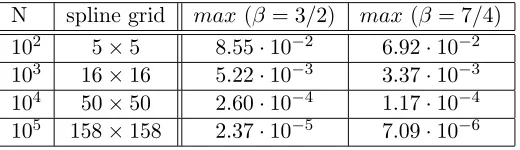
N spline grid max(β= 3/2) max (β = 7/4) 102 5×5 8.55·10−2 6.92·10−2
103 16×16 5.22·10−3 3.37·10−3 104 50×50 2.60·10−4 1.17·10−4
[image:7.595.205.465.288.363.2]105 158×158 2.37·10−5 7.09·10−6
Table 1: Maximum error using the local RBF interpolation scheme based onφ(r) =−rβ,
β= 3/2 and 7/4. Parameter values: Mmin= 100, S= 100, δ = 1.
For the thin plate spline (Table 1), the experiments confirm that the parameterδdoes not influence the error significantly. Therefore, we have chosen a nominal value δ = 1. Note that the average number of RBF knots in the local approximations approaches 140 for the larger data sets, which makes these tests particularly slow. Although an increase of Mmin was always profitable for φ(r) = −rβ, fewer knots were sufficient to achieve
nearly optimal errors forN <105. In this sense nearly optimal values of the parameter
Mmin are: Mmin = 20 forN = 102 (28 knots), Mmin= 30 for N = 103 (45 knots), and
Mmin = 60 forN = 104 (65 knots). (We have takenS =Mmin in these tests.)
Table 1 suggests the approximation order abouthβ+1, which conforms nicely to the
available theoretical results, see the comments at the end of Section 3. Note that the approximation error of the spline operatorSQav2 is O(h7) [5] and hence it is negligible for this test.
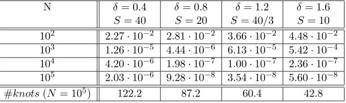
It is clear from Table 2 that in the case of multiquadrics the correct choice of the parameterδ (which clearly is related to the reciprocal of the classical multiquadric coef-ficientcin√c2+r2) is important. However, we had to choose the separation parameter
S such that δS ≤ 16 since otherwise the computation with multiquadrics turned out numerically instable. (Note that for the real world data, like those tested below in Section 5,δS must be even smaller.) The values ofMmin lower than 100 were
disadvan-tageous in our experiments for all N except N = 102. In the case N = 102, however,
Mmin = 100 delivers relatively high errors: 1.94·10−2 for δ = 0.2, S = 80, 3.75·10−2
N δ= 0.4 δ= 0.8 δ= 1.2 δ = 1.6
[image:8.595.162.509.101.205.2]S= 40 S= 20 S= 40/3 S= 10 102 2.27·10−2 2.81·10−2 3.66·10−2 4.48·10−2 103 1.26·10−5 4.44·10−6 6.13·10−5 5.42·10−4 104 4.20·10−6 1.98·10−7 1.00·10−7 2.36·10−7 105 2.03·10−6 9.28·10−8 3.54·10−8 5.60·10−8 #knots(N = 105) 122.2 87.2 60.4 42.8
Table 2: Maximum error using the local RBF interpolation scheme based on φ(r) =
−√1 +r2 for different values of δ. The spline grid is the same as in Table 1. Other
parameters: Mmin= 20 ifN = 102 and Mmin= 100 otherwise.
1.65·10−1 for δ = 1.6, S = 10. (Note that N = M
min = 100 means, in fact, that all
local approximations are the same, and, hence, our spline does not differ much from the corresponding global multiquadric approximation.) Therefore, we use Mmin = 20
if N = 102, and M
min = 100 for other N. The value Mmin > 100 may be
advanta-geous for smallerδ. For example, for N = 103 and Mmin = 200 we have 3.36·10−6 if
δ= 0.4, S = 40, and 1.26·10−5 if δ = 0.8, S= 20.
The results in Table 2 confirm that greater values ofδ tend to provide better errors. Indeed, for higherN we have to increaseδin order to obtain the best errors, even though numerical stability considerations force us to take smallerS, which in turn leads to the reduction of the number of RBF knots (see the last row of the table). For any fixed
δ, however, Table 2 shows a substantial deterioration of the approximation order as N
increases. The estimates of Section 2 do not provide a full theoretical explanation for this behavior. In particular, (11) includes the term|f|φω, whose behavior for dω→0 is
not clear to us in the case of multiquadrics.
5
Numerical Results: Real World Data
The second group of our experiments is aimed at verifying the performance of the pro-posed scheme compared with the hybrid approach introduced in [4].
To this end we consider the same real-world data sets as in [4, 5], namely, the Glacier data (GL, 8345 points), the Black Forest data (BF, 15885 points) and the Rotterdam Port data (RP, 621624 points after cleaning, see [5]). Referring to [4, 5] for the descrip-tion of these data sets, we only mendescrip-tion that GL is available from [8] and that RP has been provided by Quality Positioning Services (Zeist, The Netherlands), and it has been recorded using the QINSy software.
Note that in the first stage we use the least-squares method as described at the end of Section 2 since it consistently produced better results than interpolation for the real world data in our tests. To solve the constrained least squares problems we employ the routine DGESDD from LAPACK. (Note that the interpolation method in our implementation is also treated as special case of least squares.)
root mean square (rms) errors at the data points, the average number of RBF knots (#knots) used for the local approximations, and the computational time (time) are shown. Results obtained with the method suggested in this paper (R) are compared with the hybrid approach (H) of [4]. As in [4], we usemultiquadric RBF in these tests. The degree q of the polynomial term is 0 in all tests except RP/H, where q = 1. In the second stage we use the spline methodsRQav2 (piecewise sextic) for GL and BF and
Qav
1 (piecewise cubic) for RP, as in the respective tests in [4, 5]. The computer used for
these experiments is a Pentium 4m / 1.9 GHz / 768 MB RAM.
GL/H GL/R BF/H BF/R RP/H RP/R max 15.6m 17.8m 32.0m 30.0m 92.5cm 90.2cm
mean 1.57m 1.49m 1.39m 1.25m 5.46cm 5.23cm
rms 2.26m 2.19m 2.17m 2.00m 7.46cm 7.22cm
#knots 14.9 20.8 12.2 8.2 5.4 11.6 time 33.0sec 3.7sec 134sec 7.11sec 316sec 97.3sec
Table 3: Results for the data sets GL, BF and RP. Parameters (see [4] for the meaning of κP and κH): 1) GL. Spline grid 20×24, Mmin = 60, Mmax = 160, δ = 0.4 for
both H and R methods, κH = 105 for H, and S = 8 for R. 2) BF. Spline grid 80×80,
Mmax = 100 for both H und R methods, Mmin = 12, δ = 0.3, κH = 104 for H, and
Mmin = 3, δ= 0.4, S = 7 for R. 3) RP. Spline grid 100×281, Mmin = 3, Mmax= 100,
δ= 0.4 for both H and R,κP = 100,κH = 2·104 for H, andS= 5 for R.
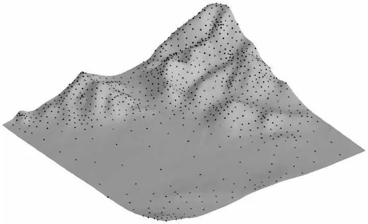
In addition to Table 3, we provide Figures 1–3 that present zooms into the same subareas of the surfaces as ones used in [4]. They are produced with MATLAB using dense grid evaluations of the spline surfaces (see [4]). The figures confirm the high visual quality of our approximations, as they show no artifical oscillation or other unnatural behaviour. Table 3 also shows that the errors for both H and R methods are comparable, whereas the computational time for the method of this paper is substantially lower.
References
[1] A. Bj¨orck, Numerical methods for least squares problems, SIAM, Philadelphia, 1996.
[2] M. D. Buhmann, Radial basis functions, Cambridge University Press, 2003.
[3] O. Davydov, On the approximation power of local least squares polynomials, in algorithms for approximation IV, J. Levesley, I. J. Anderson and J. C. Mason (eds), 2002, 346–353.
[4] O. Davydov, R Morandi and A. Sestini, Local hybrid approxima-tion for scattered data fitting with bivariate splines, manuscript, 2003.
Figure 1: Glacier test.
[image:10.595.152.513.426.646.2]Figure 3: Rotterdam Port test.
[5] O. Davydov and F. Zeilfelder, Scattered data fitting by direct extension of local polynomials to bivariate splines, Adv. Comp. Math. 21 (2004), 223–271.
[6] O. Davydov and F. Zeilfelder, Toolbox for two-stage scattered data fitting, in prepa-ration.
[7] M. S. Floater and A. Iske, Thinning algorithms for scattered data interpolation, BIT 38 (1998), 705–720.
[8] R. Franke, Homepage, http://www.math.nps.navy.mil/∼rfranke/, Naval Post-graduate School.
[9] J. Haber, F. Zeilfelder, O. Davydov, H.-P. Seidel, Smooth approximation and ren-dering of large scattered data sets, in: Proceedings of IEEE Visualisation 2001 eds. T. Ertl, K. Joy and A. Varshney, 2001, pp. 341–347, 571.
[10] A. Iske, Reconstruction of smooth signals from irregular samples by using radial basis function approximation, in: Proceedings of the 1999 International Workshop on Sampling Theory and Applications, The Norwegian University of Science and Technology, Trondheim, 1999, pp. 82-87.
[12] J. R. McMahon and R. Franke, Knot selection for least squares thin plate splines, SIAM J. Sci. Stat. Comput. 13 (1992), 484–498.
[13] R. Schaback, Reconstruction of multivariate functions from scattered data, manuscript, 1997. http://www.num.math.uni-goettingen.de/schaback/
[14] R. Schaback, Improved error bounds for scattered data interpolation by radial basis functions, Math. Comp. 68 (1999), 201–216.
[15] R. Schaback and H. Wendland, Inverse and saturation theorems for radial basis function interpolation, Math. Comp. 71 (2002), 669-681.
[16] L. L. Schumaker, Fitting surfaces to scattered data, in: Approximation Theory II eds. G. G. Lorentz, C. K. Chui, and L. L. Schumaker, Academic Press, New York, 1976, pp. 203–268.
[17] H. Wendland, Gaussian interpolation revisited, in: Trends in Approximation The-ory eds. K. Kopotun, T. Lyche and M. Neamtu, Vanderbilt University Press, Nashville, TN, 2001, pp. 427–436.
Oleg Davydov
Mathematisches Institut
Justus-Liebig-Universit¨at Giessen D-35392 Giessen
GERMANY
Alessandra Sestini and Rossana Morandi Dipartimento di Energetica
Universit`a di Firenze
Via Lombroso 6/17, 50134 Firenze ITALY