RIT Scholar Works
Theses
Thesis/Dissertation Collections
2009
Analysis of virtual environments through a web
based visualization tool
Ronald Valente
Follow this and additional works at:
http://scholarworks.rit.edu/theses
This Thesis is brought to you for free and open access by the Thesis/Dissertation Collections at RIT Scholar Works. It has been accepted for inclusion in Theses by an authorized administrator of RIT Scholar Works. For more information, please [email protected].
Recommended Citation
Analysis of virtual environments
through a web based visualization tool
by
Ronald R. Valente
September 2009
Thesis submitted in partial fulfillment of the requirements for the degree of Master of Science in
Networking and Systems Administration
B. Thomas Golisano College of Computing and Information Sciences of
ROCHESTER INSTITUTE OF TECHNOLOGY
B. Thomas Golisano College of
B. Thomas Golisano College of Computing and Information Sciences
Master of Science in
Department of Networking, Security, and Systems Administration
Thesis Approval Form
Student Name:
Thesis Title:
Thesis Committee
Name Signature Date
Committee Chair: Dr. Sumita Mishra
Committee Member: Dr. Yin Pan
I, Ronald R. Valente, declare that this thesis titled, ‘Analysis of virtual environments
through a web based visualization tool’ and the work presented in it are my own. I
confirm that:
This work was done wholly or mainly while in candidature for a research degree
at this University.
Where any part of this thesis has previously been submitted for a degree or any
other qualification at this University or any other institution, this has been clearly
stated.
Where I have consulted the published work of others, this is always clearly
at-tributed.
Where I have quoted from the work of others, the source is always given. With
the exception of such quotations, this thesis is entirely my own work.
I have acknowledged all main sources of help.
Where the thesis is based on work done by myself jointly with others, I have made
clear exactly what was done by others and what I have contributed myself.
Signed:
Date:
Abstract
B. Thomas Golisano College of Computing and Information Sciences
Department of Networking, Security, and Systems Administration
Masters of Networking and System Administration
by Ronald R. Valente
September 2009
Virtualization is gaining popularity in corporations as well as academia. This technology
provides a large return on investment by providing the ability to consolidate hardware
servers into smaller, more efficient virtual machines (VM). With a seemingly negligible
cost to deploy a new virtual machine when compared to deploying a physical server, more
and more virtual machines get deployed. However, as the number of virtual machine
increases, the task of managing and keeping track of them becomes exceedingly
cumber-some. With advanced visualization techniques and real-time analysis of virtualization
environments, the control over virtual machine sprawl will become more manageable
and thus improving virtual environment efficiency.
This thesis describes the development of a novel web-based visualization tool for the
virtual environment. With this tool, it is possible to better monitor the environment and
control the VM sprawl. This tool provides the potential to optimize the environment and
maintain an optimal level of performance for each virtual machine in the environment.
I would like to thank the following people who have helped me not only through this
thesis but my educational career...
My family and friends have been a continued source of support.
Dr. Sumita Mishra has been a great influence whose energy and enthusiasm throughout
this entire project helped me stick with it.
Dr. Luther Troell for the guidancehe provided my throughout my undergraduate and
graduate career at RIT.
Dr. Yin Pan who had a fantastic way of presenting material during courses which made
everything more interesting than it should have been.
Declaration of Authorship ii
Abstract iii
Acknowledgements iv
List of Figures viii
List of Tables ix
1 Introduction 1
1.1 Virtualization Background . . . 1
1.1.1 Benefits of Virtualization . . . 1
1.1.2 Challenges of Virtualization . . . 2
1.2 Need for Tools and Analysis . . . 2
1.3 Work Presented . . . 3
2 Literature Review 4 2.1 Overview . . . 4
2.2 Virtualization . . . 4
2.3 Storage . . . 6
2.4 Visualization . . . 7
2.5 Conclusion . . . 8
3 Methodologies 9 3.1 Overview . . . 9
3.2 Environment . . . 9
3.3 Purpose . . . 11
3.4 Limitations . . . 11
3.4.1 Assumptions . . . 12
3.4.2 Validity . . . 12
3.4.3 Growth . . . 13
3.5 Procedure . . . 13
3.5.1 Data Collection. . . 14
3.5.2 Visualization . . . 14
3.6 Conclusion . . . 15
4 Web Application 16 4.1 Overview . . . 16
4.1.1 Database . . . 17
4.1.2 Interface. . . 18
4.1.3 Dashboard . . . 18
4.1.3.1 Available Counters. . . 18
4.1.3.2 Host Summary . . . 20
4.1.3.3 Array Summary . . . 21
4.1.4 Navigation . . . 21
4.1.5 Hosts View . . . 23
4.1.6 Storage Array View . . . 25
4.2 Analysis . . . 26
5 Results & Discussion 28 5.1 Overview . . . 28
5.2 Host Analysis . . . 28
5.2.1 CPU Usage . . . 29
5.2.2 Memory Usage . . . 32
5.2.3 Disk Usage . . . 35
5.2.4 Counter Overview . . . 36
5.2.5 Host Data Source Correlations . . . 37
5.3 Storage Analysis . . . 38
5.3.1 Utilization. . . 39
5.3.2 Queue Length. . . 40
5.3.3 Response Time . . . 41
5.3.4 Throughput . . . 42
5.3.5 Bivariate Throughput . . . 43
5.3.6 Bivariate Queue Length . . . 43
5.3.7 LUN Performance . . . 45
5.3.8 Disk Performance. . . 46
5.4 Conclusion . . . 47
6 Conclusion 48 6.1 Overview . . . 48
6.2 Web Application . . . 48
6.3 Host Analysis . . . 49
6.3.1 Access Reduction . . . 50
6.3.2 Monitoring . . . 51
6.4 Storage Analysis . . . 51
7 Recommendations 52 7.1 Future Work . . . 52
7.1.1 Collection Improvements. . . 52
7.1.2 Available Counters . . . 53
7.1.3 Realtime Analysis . . . 53
7.1.4 Flexible Visualization Code . . . 53
7.1.5 Pure Ruby Implementation . . . 53
7.1.6 Notifications . . . 54
7.2 Conclusion . . . 54
A Key Terms 55 A.1 Virtualization . . . 55
A.2 Programming . . . 55
C Host Data Collection 57
C.1 ESX Host . . . 57 C.2 esxtop configuration . . . 58
D Data Summarization 59
D.1 Host Summarization . . . 59 D.2 Array Summarization . . . 61
E ESX Host Data Collection 63
E.1 VMware API Perl Script. . . 63
F Web Application Database Schema 68
F.1 Schema Design . . . 68
G JMP Scripts 70
G.1 LUN Bubble Plot . . . 70
H Storage Array Collection Scripts 71
H.1 Storage Data Collection Script . . . 71
2.1 MRTG Graphing Output[1] . . . 7
2.2 RRDtool Graphing Output[2] . . . 8
3.1 VMware Cluster Rack Layout . . . 10
3.2 Cluster and Storage Rack Layouts . . . 10
4.1 veViz Dashboard . . . 19
4.2 veViz Host Summary Detail . . . 20
4.3 veViz Array Summary Detail . . . 21
4.4 veViz Navigation Menu . . . 21
4.5 veViz Host Selection . . . 23
4.6 veViz Host Detail . . . 23
4.7 veViz Host Legend . . . 24
4.8 veViz Host Memory Usage . . . 24
4.9 veViz Array Selection . . . 25
4.10 veViz Array Detail . . . 26
4.11 veViz Array Legend . . . 26
5.1 CPU Usage (MHz) . . . 29
5.2 Host CPU Usage by Host . . . 30
5.3 Host CPU Usage Range . . . 31
5.4 Host CPU Time Series . . . 31
5.5 Memory Usage (%) . . . 32
5.6 Host Memory Time Series . . . 33
5.7 Overall Memory Usage . . . 34
5.8 Disk Usage (KB/sec) . . . 35
5.9 Counters vs. Timestamp by CPU Level . . . 36
5.10 CPU Memory and Disk Scatterplot Matrix . . . 37
5.11 Service Processor Distributions . . . 39
5.12 Bivariate: Utilization & Total Throughput. . . 43
5.13 Bivariate: Total Throughput & Queue Length. . . 44
5.14 Bivariate: Response Time & Queue Length . . . 44
5.15 Bivariate: Flush Ratio & Queue Length . . . 45
5.16 LUN Queue Length, Throughput, and Response Time . . . 46
5.17 Individual Disk Bubble Plot . . . 47
3.1 Virtual Environment Components . . . 10
3.2 Virtual Environment Hardware Specifications . . . 11
4.1 Available Environment Counters . . . 19
5.1 Host CPU Counter Moments . . . 29
5.2 Host CPU Level Color Legend . . . 30
5.3 Host Memory Counter Moments . . . 32
5.4 Host Memory Level Color Legend . . . 34
5.5 Host Disk Counter Moments . . . 35
5.6 Storage Array Objects . . . 38
5.7 SP A/B Array Utilization Moments . . . 40
5.8 SP A/B Array Utilization Quantiles . . . 40
5.9 SP A/B Array Queue Length Moments . . . 40
5.10 SP A/B Array Queue Length Quantiles . . . 41
5.11 SP A/B Array Response Time Moments . . . 41
5.12 SP A/B Array Response Time Quantiles. . . 41
5.13 SP A/B Array Throughput Moments. . . 42
5.14 SP A/B Array Throughput Quantiles . . . 42
7.1 Data Rollup Policy . . . 53
F.1 veViz Summary Schema . . . 68
F.2 veViz Master Schema . . . 69
1
Introduction
1.1 Virtualization Background
Virtualization has been around since the early 1980s. Virtualization was not extremely
efficient or practical back when it was conceived. It took a large amount of time and
effort to instantiate a single virtual machine. There was not a demand for virtualization
because of the learning curve and additional steps required to utilize it. All that has
changed substantially since then and now virtualization has made a surge into both the
corporate and academic realms.
1.1.1 Benefits of Virtualization
By leveraging virtualization, one has the capability to isolate an operating system
in-stance without requiring dedicated hardware for each inin-stance. Having this flexibility
provides the user with the ability to increase utilization of each hardware machine, thus
allowing each hardware server to run at a higher level of utilization resulting in lower
amount of servers needed overall. Ultimately this reduction in number of servers should
be able to create a more cost effective and easier to maintain datacenter.
1.1.2 Challenges of Virtualization
With all of the positive effect that virtualization has made on corporate entities and
academia, it is hard to even notice the drawbacks at times. For instance with large virtual
environments, the ability to create and deploy a virtual machine is easy but keeping
track of all the virtual instances can be challenging to say the least. Keeping track of
these virtual machines is so challenging that there is an outbreak of virtual machines
in virtual environments. This outbreak can be dedicated entirely to the difficulty to
monitor and manage the purpose of virtual machines and the usage. It is not as simple
as checking if the virtual machine is on or off. This problem ripples across the entire
virtual environment because the number of virtual machines directly correlates with the
performance of the environment as a whole.
1.2 Need for Tools and Analysis
Virtualization has been such a driving force in the information technology field, the
ability to control the virtual environment is becoming harder as the environments grow
in size and capability. There needs to be a revolutionary method for the analysis of
a virtual environment which will permit a deeper look into the environment for better
optimization and efficiency. Considering all of the variables that contribute to the overall
performance of a virtual environment it would only make sense to run a multivariate
analysis of the environment to determine interactions, if any. If any interactions are
found, one may find the potential to improve performance without additional hardware
just by optimizing variables within the bounds of the given environment.
Virtualization and the act of abstracting an application or operating system from the
hardware is not a new idea by any stretch of the imagination. That being said using
virtualization to improve system utilization, reduce power consumption, and increasing
the flexibility and redundancy of the environment are just some of the reasons why its
popularity is increasing so rapidly. No one solution is perfect, and leveraging
virtual-ization has its caveats. Most importantly is the complexity of monitoring the system.
There are now multiple layers of performance that must be monitored. On top of that
storage is now centralized which can now be a bottleneck in some operations. The ability
to flexibly and efficiently monitor these virtual environments is extremely important to
1.3 Work Presented
This thesis uses combination of programming, system administration, and statistical
analysis to provide a set of methods to perform in-depth analysis of virtual environments.
Data is collected using an optimized polling mechanism and save all the information into
a relational database. Once the data is stored into a database further analysis can is
performed via JMP, a statistical package. Statistical analysis of virtual machines and
storage utilization using control charts and other statistical methods will is implemented.
Each of these methods will is represented in a coherent manner to increase the readability
2
Literature Review
2.1 Overview
There are three overarching topics that have a role in virtual machine sprawl,
virtual-ization, storage, and efficiency. By monitoring the virtualization and storage aspects of
a virtual environment then and only then can virtual machine sprawl be tracked. When
looking into a typical virtual environment deployment, it is important to state that there
usually is not one admin. There are multiple admins in charge of different aspects of the
system. For example, one admin would handle the storage, while another admin would
monitor and control the ESX servers. This segmentation can create a disconnect when
it comes to overall efficiency between the virtualization/host side and the storage area
network side on the environment. With proper analysis and visualization it is possible
to close the gap between the two main aspects of a virtual environment and get a better
handle on virtual machine sprawl.
2.2 Virtualization
Virtualization has been an extremely popular topic lately due to its many touted
advan-tages with seemingly minimal disadvanadvan-tages. Virtualization has been made out to be
such a great technology that any disadvantaged is out-weighed by the massive amount
of advantages. These miniscule disadvantages in an environment that is in its infancy
can evolve into severe problems in the future. The major disadvantages for a virtual
environment is directly related to one of its advantages, deployment. With a virtual
environment, deploying the server consists of right clicking and selecting the new virtual
machine operation. After completing the wizard and a few minutes go by, you have a
brand new server ready to work on. The speed and ease of deployment has made the
cost of server deployment disappear, at least to the end-user or specific server admin.
The virtual machine admin on the other hand knows there is a specific cost to every
VM and each cost is different based on the resource utilization of that VM.
With regards to the ease of deployment there is one major result, the over abundance of
VMs in a virtual environment. This excessive creation of VMs creates a set of issues in
the environment that may not have been an issue without the use of VMs. By having so
many VMs running, manageability decreases, performance of each VM decreases, and
storage availability decreases. The term for this proliferation of virtual machines in a
virtual environment is called VM Sprawl.
There has been a few technologies that have been developed to slow the reduction in
resources by creating new VMs in a virtual environment. Some of these technologies
that have been developed cost more money or require more administration overhead
to implement. VMware has introduced a technology in VMware Workstation2 which
leveraged the copy on write method to implement what they calllinked clones. A group
of engineers from IBM proposed a solution for VM sprawl which involved converting the
current VM format to a proprietary format which increase the ability to compress and
share data between VMs to lower storage utilization [3]. This solves one aspect of the
VM sprawl issue but fails to handle resource utilization creep.
By leveraging the visualization of the virtual environment as opposed to using a
propri-etary VM disk format it should be possible to implement this solution without a change
up-front to the environment. The visualization of the entire environment will give all
users of the environment more insight on the usage of each component and not just the
pieces they user every-day.
2
2.3 Storage
As technology improvements keep increasing with regards to virtual environments there
becomes a greater demand for storage area networks, or shared storage. These storage
networks enable a great deal of functionality but add a layer of complexity to the entire
virtual network. Traditionally there was a separate staff for storage in charge of just
that. After virtualization became so important in many corporations, having a separate
team just for storage became impractical. That being said, storage and system admin
positions have merged together to generate a virtualization environment admin. These
admins are in charge of the virtualization servers and the storage dealing directly with the
virtualization hosts and nothing else. The admins sometimes can handle the individual
guests but with regards to vm sprawl, it is a larger issue if there is a large user-base.
The more people with access to the system there is a greater chance to have a serious
issue with VM sprawl.
There are two major facets that come with virtual environments related to storage.
These facets combine the performance of the array with the overall storage usage of the
array. Both of these metrics are used to determine if/when more storage needs to be
purchased. Currently some storage area networks have a type of monitoring solution
that is shipped with the product or as an add-on. A manufacturer analysis mechanism
is not necessarily a poor choice, but the integration between that and the virtualization
servers and the virtual machines themselves is not possible. This combination is where
the power of monitoring and visualization can be realized.
So there are multiple factors when it comes to monitoring the storage of a virtual
envi-ronment. The main pieces that makeup storage in a virtual environment are over storage
utilization, virtual machine disk size, and used space in the VM. By monitoring each of
these variables as well as virtual machine and the virtualization servers, the admin can
get a greater understanding of the environment and the interactions between all of its
2.4 Visualization
Data collected about virtual environments, or any system based environment is very
important. The ways to go about collecting the data are all very similar. Usually a
software development toolkit (SDK) or scripted command line utility is used to collect
the data and store it either to a file, database, or directly to a filesystem hierarchy.
Visualization of that data was very ad-hoc, reports were generate when needed. Initially
this solution was suitable for the requirements.
As systems became more complex and and the data collection became more efficiency
it was possible to collect more information about the environment. Not only was it
possible to get more data from each component, it was also more efficient and faster as
well. The requirement to collect data, and retrieve it on the fly for report generation
was increasing rapidly.
Figure 2.1: MRTG Graphing Output[1]
Visualization of data within systems and network environments has been very
impres-sive over the years. The need for visualization is an obvious one and the development
into applications and application programming interfaces (APIs) are a great example of
this need. The rapid progression of Tobias Oetiker’s graphing and data storage methods
are testament to this statement. Tobias developed a product calledMulti Router Traffic
Grapher (MRTG) and it was a simple but effective mix of data collection and
visualiza-tion in the same product [1]. It queried routers over the simple network management
protocol (SNMP) and graphed the output. A snapshot of the output is in Figure2.1.
After a while it was apparent that MRTG did not have enough flexibility to complete
other visualization tasks, which it was not designed for. Tobias developed an application
calledRRDtool, RRD stands for round robin database. RRDtool was not actually used
Figure 2.2: RRDtool Graphing Output[2]
the administrator and not provided by the developer for maximum flexibility [2]. A
screenshot of what can be done with RRDtool is shown in Figure2.2.
While RRDtool had increased flexibility when compared to MRTG it was still limited
for the use in this thesis. In order to support a web application and analysis in JMP a
relational data was required. Storing the data in a relational database allowed for quick
access to very large amounts of data.
2.5 Conclusion
When combining data collection from multiple sources and visualization visualization a
unique challenge crops up. It is important to determine the most appropriate tools for
this job. In this case MySQL[4] was used because of its speed and efficient handling of
large data sets. The graphing methods would need to be extremely flexible considering
the different data types and varying amounts of data passed to it. Using amCharts
[5] proved to solve all of those problems because it understands XML and can create
3
Methodologies
3.1 Overview
Multiple visualization techniques were implemented to improve the usefulness of the
data collected. In order to convey the importance of understanding each component
of a virtual environment as well as their interactions between each other a platform
that could be simple yet descriptive was used. Improving the visualization of a virtual
environment will increase the manageability, which should in turn increase the ability to
reduce the number of virtual machines and/or improve performance of the environment
as a whole.
3.2 Environment
In order to develop a procedure to analyze and maintain a virtual environment, a complex
environment was used for this thesis. All of the data collected for this thesis was polled
from a production network in use 24/7. There are about 500 virtual machines and
growing within this virtual environment.
While every virtual environment is different, there are similar aspects within each and
every one. Every environment can be broken down to three major parts; storage, servers,
and network/fabric. The environment consisted of multiple servers interconnected with
two different types of networks. One network used solely for the shared storage and
another network used TCP/IP traffic. The table 3.1 lists the hardware used in the
environment.
Component Classification Quantity
HP DL 380 G5 Server 43
EMC CLARiiON CX4-240 Storage 1
Cisco Catalyst 3750 Network 4
Cisco MDS 9134 Fabric 4
Table 3.1: Virtual Environment Components
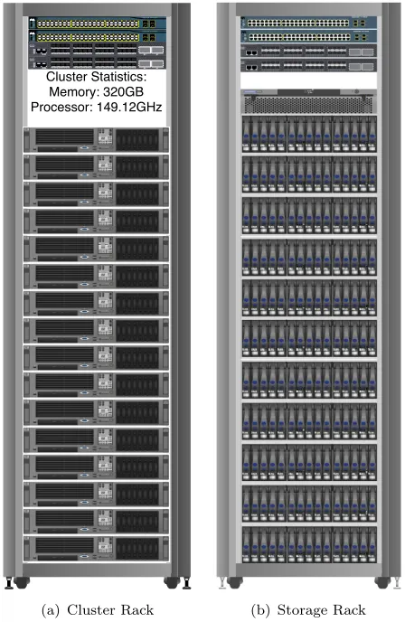
A full VMware cluster is made up of 16 servers in the environment. There are redundant
switches at the top of each rack, two Cisco MDS fiber channel switches and two Cisco
3750 multi-layer switches. The table3.1defines a a fourth set of switches which are used
to the EMC array connection into the environment. The layout of a rack used in this
virtual environment cluster is shown in Figure3.1
Figure 3.1: VMware Cluster Rack Layout
Catalyst 3560SERIES SYST MODE SPEED DUPLX POE STATRPS 1X 18X 17X 16X 2X 15X 31X 32X 34X 33X 47X 48X
1112131415161718192021222324252627282930313233343536373839404142434445464748 12345678910
1
PoE-48
3
2 4
CONSOLEMGMT 10/100 MDS 9134 MULTILAYER FABRIC SWITCH
STATUS P/SFAN
DS-C9134-K9LINKACT1234567891011121314151617181920212223242526272829303132 10GE1 10GE2
CONSOLEMGMT 10/100 MDS 9134 MULTILAYER FABRIC SWITCH
STATUS P/SFAN
DS-C9134-K9LINKACT1234567891011121314151617181920212223242526272829303132 10GE1 10GE2
Catalyst 3560SERIES SYST MODE SPEED DUPLX POE STAT RPS 1X 18X 17X 16X 2X 15X 31X 32X 34X 33X 47X 48X
1112131415161718192021222324252627282930313233343536373839404142434445464748 12345678910
1
PoE-48
3
2 4
CONSOLEMGMT 10/100 MDS 9134 MULTILAYER FABRIC SWITCH
STATUSP/S
FAN
DS-C9134-K9LINKACT1234567891011121314151617181920212223242526272829303132 10GE1 10GE2
CONSOLEMGMT 10/100 MDS 9134 MULTILAYER FABRIC SWITCH
STATUSP/S
FAN
DS-C9134-K9LINKACT1234567891011121314151617181920212223242526272829303132 10GE1 10GE2
RTP-VNAP-02 RTP-VNAP-01 RTP-VNAP-03 RTP-VNAP-05 RTP-VNAP-06 RTP-VNAP-08 RTP-VNAP-07 RTP-VNAP-10 RTP-VNAP-09 RTP-VNAP-11 RTP-VNAP-12 RTP-VNAP-13 RTP-VNAP-14 RTP-VNAP-16 RTP-VNAP-15 RTP-VNAP-04 Cluster Statistics: Memory: 320GB Processor: 149.12GHz Cisco 3750 Cisco MDS 9134 Cisco MDS 9134
Cisco 3750
[image:21.596.203.427.386.730.2](a) Cluster Rack (b) Storage Rack
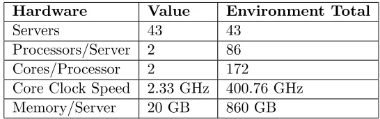
To dive deeper into the environment used we can combine what we know about the
servers used within the environment and compile a maximum resourcelevel with regards
to the environment as a whole. Shown in the table 3.2, we now have an environment
resource total.
Hardware Value Environment Total
Servers 43 43
Processors/Server 2 86
Cores/Processor 2 172
Core Clock Speed 2.33 GHz 400.76 GHz
[image:22.596.179.452.164.250.2]Memory/Server 20 GB 860 GB
Table 3.2: Virtual Environment Hardware Specifications
By creating compiling these numbers we now have a ceiling to compare the results to.
Due to the nature of virtual environments and their inherent flexibility with back-end
resources, it is certain that it will change. When the back-end of the environment
changes, either add more servers or replace old servers, the resource ceiling will change.
3.3 Purpose
The purpose of this thesis was to provide a set of tools that will allow for the
enhance-ment of the manageenhance-ment of virtual environenhance-ments. The enhanceenhance-ments are in the form
of improved monitoring via statistical analysis between each of the components that
makeup a virtual environment. To further the impact of the data collected during the
monitoring process of a virtual environment, different visualization techniques were used.
3.4 Limitations
There will inevitably be limitations in this thesis project due to the scope of the project.
Certain limitations will be more prominent only due to the factor of time. Some of
these limitations that may arise will be regarding speed, encrypted communication, and
number of potential visualization platforms.
Considering the most important process in this project is regarding data collection,
analysis, and visual representation of a virtual environment, that will be the highest
priority. The data collection itself can yield a great deal of information, if there is
too much data initially, a pruning method or random sampling process will need to be
Once data collection and analysis is complete some of these initial limitations, if they
exist, will be addressed. For example, with regards to number of visualization platforms,
after one platform is functional, then and only then will a second platform be explored
and implemented, time permitting.
There will be many different processes that are dependents of analysis of the virtual
environment. That being said, if one or more of these processes experience any latency,
it will slow down the entire analysis of the process. If the analysis takes longer than
usual, optimizations will be implemented as needed and time permitting.
3.4.1 Assumptions
There were some assumptions that had to be made during the course of this thesis. These
assumptions were necessary in order to ensure the accurate interpretation of the data
collected. It was assumed that the storage array being polled was an EMC2 CLARiiON
storage array using the Navisphere1 manager. Secondly it was assumed that VMware2
was ESX3 was used on all the virtual environment servers.
3.4.2 Validity
The data collected and analyzed for this thesis is strictly applicable only to this
envi-ronment at the time of the data collection. Due to the fast growth of the envienvi-ronment
outlined in section 3.4.3 it would be unlikely for data collected in the past to apply
to a current environment. That being said using past data would prove useful when
compared to current results to detect trends or improvements in the environment.
1
EMC2 Software Management 2
Virtualization Technology Leader 3
3.4.3 Growth
Growth can be defined in two ways with regards to a virtual environment, back-end
growth and front-end growth. Back-end growth would occur when more resources were
required after analysis was completed and determined that no virtual machines could
be consolidated. Other reasons why back-end growth could occur is when servers fail,
and new servers which are more powerful replace the older servers.
Front-end growth on the other hand is referring to virtual machines, as number of
virtual machines increase, storage, memory, and cpu resources are consumed. When
virtual machines are created without bound, these resources can be consumed at an
astonishing rate.
The ideal option would not be to prevent growth within a environment but control and
manage the changes and additions to the environment. Processes can be put in place to
track the growth of the environment. With this in place it would be easier to manage
the changes within an environment and to catch problems before they occur.
3.5 Procedure
By using a custom architected web application along with a statistical approach
lever-aging detailed visualization one should be able to improve the performance of virtual
machines and efficiency of the storage within a virtual environment. The improvements
will be measured by disk usage, CPU usage and memory usage.
Data collection will run continuously pulling from ESX servers as well as the storage
sys-tem in a virtual environment. The data collected will be stored in a relational database
that can be leveraged by many applications. By utilizing statistical approaches outlined
in JMP Start Statistics[6] one should be able to improve the virtual environment. Once
the data is collected, the analysis should be able to identify any potential trends and
interactions. Once the analysis of the data is complete the visualization of the results
3.5.1 Data Collection
Both the servers and storage have their own proprietary collection methods, each with
access restrictions and separate application programming interface (API). Each of the
devices collect data at similar intervals, the servers get polled every 5 minutes and the
storage gets polled on an average of every 3 minutes. The data collected within the
devices gets stored during the data in a persistent data store and will be polled at the
end of every day through the API.
Each component required the use of a different API2 leveraged from a separate script.
Each script or set of scripts depending on the component of the environment added the
data collected for that day into a relational database. The database used for this thesis
was MySQL3
The VMware API has a great deal of features regarding performance data collection.
Details can be collection ranging from IOPS on a server to IOPS on a VM level. The
level of detail is an advantage as well as a disadvantage. In order to work through the
complexity of the API there are some techniques that must be used. For example when
collection data from a continually polled instance like a vCenter server it is import to
collect only the data necessary and using all the data collected [7]. If the data that is
collected is not used then the time taken to collect the data was lost and thus decreases
the perceived performance of the web application, not to mention the amount of storage
used will increase.
3.5.2 Visualization
Disregarding the topic of virtualization for the time being, it has always been the goal of
network and system administrators alike to collect data about their systems. The data
collected allowed the admin to get a better idea about how their systems were operating.
Having past data to compare current operating conditions against aids in the detection
of potential problems and other degradations in systems. With regards to virtualization,
effective data visualization is extremely important. There would be no effective way to
monitor a virtual environment without data collection about the virtual machines, the
virtualization hosts, and the storage system.
2
Application Programming Interface
Typically a virtual environment will be polled during a normal duty cycle and not
much experimentation is performed ahead of time. That being said one of the most
effective methods to visualize the data in a production environment is to use a time
series representation [6]. The reason this method works so well is because usually when
in production, there is little room for experimentation. The time series representation
will allow one to potentially forecast future trends to have a better idea of growth
regarding the virtual environment.
Visualization should not stop at time series representations of data, especially with
vir-tual environments. There is more information that can be determined from the data
that is collected. Some of the other visualization techniques that can be used are bubble
plots, control charts, and overall distributions of the data. All of these methods have
their own advantages and can all be used to gain a greater understanding of the
en-vironment as a whole. One visualization technique to find all the possible corrections
in the virtual environment called the scatterplot matrix in the JMP software would be
beneficial for the analysis[8]. By finding correlations between the data sources within a
component we can then optimize our analysis by knowing more information about the
environment.
3.6 Conclusion
By leveraging effective visualization of data using both a web application and the JMP
product, there is much more value that can be drawn from the raw data. By using
some of the JMP platforms outlined in [9] there are many meaningful types of output
we can provide about a virtual environment. The output that JMP will provide will
offer a more detailed and customizable viewcompared to the web application. Aside
from being more flexible and agile, JMP requires an additional piece of software with
its own learning curve. That being said the web application offers a great way to have
4
Web Application
4.1 Overview
As stated in section3.1there are two major parts to this thesis, data collection and data
visualization. The data collection was handled by separate scripts for each component
of the virtual environment and the data visualization was handled by a custom web
application and JMP. The following section describes the custom web application written
for this thesis.
A web application for ongoing analysis allows for a platform independent approach for
rapid analysis of a virtual environment. Not only is this an efficient approach to provide
admins with the most up-to-date data but it is also a fantastic way to deliver the results
to a wide range of users as efficiently as possible.
Knowledge of virtualization has become mandatory within the field of system
administra-tion. It is important to not only posses the knowledge of building a virtual environment
but the ongoing maintenance and management of one. By providing a set of tools and
procedures it is then possible to manage a very large environment with ease compared
to a manual style of management.
Monitoring a virtual environment is a very important task in order to maintain optimal
performance. In order to effectively and accurately monitor a virtual environment it
must be a quick operation to initially see the health of the environment. If further
investigation is required then a more in-depth process can be documented and easily
performed.
Providing a web application to offer a way to monitor the virtual environment gives
the administrators insight into the environment. By simply having the web application
available to the administrators, they have the ability to quickly discover where issues
exist within the environment without time consuming analysis. This allows the
admin-istrators to start debugging quicker. If the web application is used on a regular basis
it would even be possible to catch problems before they start and pro-actively perform
maintenance on the environment.
The web application is namedveViz which stands forvirtualenvironmentVizualization.
The web application itself is a front-end to the data collection methods. These methods
are supported by a few backend scripts which get called from a cron1 job. By using a
front-end which reads directly from the database which is filled via different backend
scripts, it provides the ability to use the native API of each component of the virtual
environment. Using the native API where available is the best choice when collecting
data from a virtual environment because it enables the admin to collect the data with
the most detail possible. This was a much better approach than the initial option of
using theesxtopcommand. The VMware esxtopcommand was resource intensive and
required communication to every ESX server. Using the API instead allows a central
collection point from the vCenter server itself.
4.1.1 Database
The database schema was designed to support both a web application as well as more
in-depth analysis via JMP. That being said, the amount of normalization was minimal
due to the complexity it would add to the third party analysis. There were four tables
used for the development of the application, two for summarizations of the data and two
for raw data collected.
Summary Data Raw Data
array summaries storage arrays
host summaries hosts
The summary tables are used for the dashboard of the application and are appended to
via a script within the web application detailed in AppendixD. The other two tables are
master tables that receive data directly from their respective sources. The VMware ESX
API fills the hosts table via a perl script outlined in AppendixEand the storage arrays
table gets filled via a CSV import using the EMC2 Navisphere Analyzer CLI via a script
detailed in Appendix H.
Refer to Appendix F.1 for the detailed database schema design.
4.1.2 Interface
The web application itself is modular considering the fact that it brings together each
piece of a virtual environment to one concise monitoring interface. The interface was
designed to be clean and simple without many options to limit confusion. The three
major pieces of the web application are the dashboard, hosts view, and storage array
view. Each of the pieces of the web application enables their own specific purpose to
allow for better visualization of that specific component in the virtual environment.
4.1.3 Dashboard
The application has a home page view that quickly will summarize the most important
factors of the virtual environment. The dashboad of the web application allows for
a summary the virtual environment based on a pre-calculated average of each value
collected that that component. The dashboard page updates each day when the cron
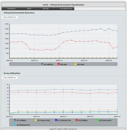
script is enabled. A full page overview of the dashboard is shown below in Figure 4.1.
The dashboard consists of two major aspects of the virtual environment, the storage and
the servers. It summarizes both of these in an individual graph for each section of the
environment averaged out for each day. For example, the server side of the environment
is made up of 43 servers, these servers are polled every 5 minutes. The dashboard takes
every value for each server and averages them for that day. This simple front page gives
a very brief overview of the operational characteristics of the environment as a whole.
4.1.3.1 Available Counters
There are a set of counters that were used most prominently to determine the operational
Figure 4.1: veViz Dashboard
the storage array and ESX servers and are represented in Table 4.1. Having different
counters was done mainly because of API restrictions of the respective environments.
Array Counters
Counter Unit
Utilization Percent Queue Length Integer Response Time ms
Host Counters
Counter Name Unit
CPU Usage MHz
Memory Usage Percent
[image:30.596.110.522.83.502.2]Disk Usage KB/sec
Table 4.1: Available Environment Counters
Each environment consisted of 3 main counters which summarize the operation of the
represent the performance of that environment well. A more detailed view of the
en-vironment can be gained by reviewing all the counters available for that enen-vironment.
This would not be possible within the web application due to performance reasons.
4.1.3.2 Host Summary
The host summary polls the VMware vCenter database for the counters in Table 4.1
which are collected nightly. These three counters are the best counters available at the
ESX host level to determine the performance of each ESX host within the environment.
4.1.3.3 Array Summary
The counters used for the dashboard are pulled from the database using each service
processor (SP) as the object to query. The service processor handles all the transactions
on a storage array so it is a good place to start when querying the usage of a storage
environment. That being said, there are many other objects in a storage array where
performance contention issues may occur. Analysis of these objects are available in the
storage tab of the web application described in Section 4.1.6. Table 4.1shows the three
main counters used in the dashboard view for the overview analysis.
Figure 4.3: veViz Array Summary Detail
4.1.4 Navigation
Navigation is a very important aspect of any application. Without a simple navigation
tree it would be difficult for a wide audience to use any application. Considering that
this application should be able to be used by anyone that is interesting in the virtual
environment, there should be a rock solid navigation implemented. Below in Figure4.4
shows the navigation used in the web application.
Figure 4.4: veViz Navigation Menu
Along with the dashboard for the web application there are detailed views for both hosts
The virtual machine tab is disabled for the time being, until data rollup is implemented
it would not be practical to implement collection performance data for each virtual
4.1.5 Hosts View
A detailed view of each host is possible within the web interface. By providing the
option to drill down to each individual host allows for a better understanding of each
host. Not only can an individual hosts details be viewed but the user can select any
available date range to see anything from daily trends and beyond. These options are
selected in a fashion as depicted in Figure4.5.
Figure 4.5: veViz Host Selection
Once the users selects the host and time period which is of interest after submitting the
values to the application it will return the desired query. For every host that is selected
three counters are displayed by default. These counters can be hidden to see a better
representation of a specific counter. Figure 4.6is the display of all values on one chart.
Figure 4.6: veViz Host Detail
Figure 4.7: veViz Host Legend
If you want to only view memory usage uncheck the boxes in the legend for the chart.
By doing this the chart will only the data that is under the series that is checked. The
chart will redraw automatically using the new data set without having to reload the
entire page. Below in Figure 4.8shows the level of detail that is gained for the memory
[image:35.596.109.526.261.477.2]counter by limiting it as the only data on the graph.
4.1.6 Storage Array View
The storage array used in this virtual environment was anEMC2 CLARiiON CX4-240,
there is a command line interface which allows for secure communication between a
EMC2 provided application and the array. On top of that the collection daemon can be
set to run indefinitely or for a set amount of days. Once we download the data for each
day there is some post processing that needs to be done before we can bring it into the
web application’s database. We must sanitize the date format to be compatible with
the MySQL default format, on top of that we need to remove the first line of the file
because those are the column names. Once this is done we are ready to import the data
into the database.
The web application itself reads the contents of the database just like the Hosts selection
screen, this allows for the form to be dynamically generated based on the content of the
database. By dynamically generating the form fields the web application could then
support any number of storage arrays just be changing the back end scripts to collect
the data along with the database schema. A view of the selection screen is shown below
in Figure 4.9.
Figure 4.9: veViz Array Selection
Once major difference with the storage array and the hosts selection screen is that you
now have the ability to view a certain counter. By doing this there was little post
processing that needed to be done on the storage arrays data. Once the data is in the
database we can view each counter individually. Below in Figure 4.10 shows the SP A
Figure 4.10: veViz Array Detail
In contrast to the host detailed view, with the storage arrays view only one counter
is available for viewing due to the increase amount of data that is collected. It is not
feasible to have a great deal of data within these charts because the readability and
speed of the chart generation decreases dramatically.
Similar to the hosts view, the legend displays the counter that is being represented in
the graph above and the ability to hide the line.
Figure 4.11: veViz Array Legend
4.2 Analysis
The host portion of the web application accomplishes two tasks, providing a daily
sum-mary of the virtual environment with regards to the three counters being polled as well
as a detailed analysis of each host being monitored. By offering the two levels of details
trouble spots can be found using the daily summary and then investigated in great detail
on a host-to-host basis.
In order to keep the web application performance and resource utilization at a reasonable
web application has two parts as stated in4.1.3 and 4.1.6. Each of these sections play
an important role in the ongoing analysis of the storage component.
While the web application is a fantastic way to dynamically generate charts on the most
current data, there is greater detail that can be learned if a move in-depth analysis is
done. The application used for the analysis is JMP2
2
5
Results & Discussion
5.1 Overview
The two pieces of the environment which were monitored were the ESX servers and the
EMC storage array. Each of these parts of the virtual environment are integral pieces
that must be maintained. The host statistics pulled via the API consists of the three
major counters. The counters that were polled via the API from the virtual environment
are listed in Table4.1. In order to improve the visualization of the data post-collection
modifications have been made within JMP.
A detailed view into the environment along with the web application allows for the
abil-ity to drill-down into the environment on trouble spots. By having this magnifying glass
on top of using the web application an administrator can potentially track down
prob-lems which have not manifested by failure and remedy them without the end-usereven
knowing there was a problem in the first place.
5.2 Host Analysis
Knowing a virtual environment is extremely important, especially when monitoring the
performance and capabilities of the environment. There should be an inventory of
com-ponents within the virtual environment consisting of; number of servers, processors in
each server, cores per processor, and memory per server. Having this will provide a
baseline of the environment that can be tracked as well as used to predict capacity
re-quirements when more servers are needed. All that being said, refer to Table3.2for the
information on the virtual environment used for this thesis. The last column in Table
3.2 shows the summation of all the available resources within the environment, we can
use these numbers to compare our findings to. The data sources that were polled from
each host were CPU usage (Section5.2.1), memory usage (Section5.2.2), and disk usage
(Section 5.2.3).
5.2.1 CPU Usage
CPU usage within a virtual environment is extremely important. CPU resources are
important to have plenty extra of because virtual machines can have a spike in CPU
usage at any time. The quartiles shown in Table 5.1show that while normal operation
is around 1 CPU in total MHz, spikes can jump to a much higher extreme. While trends
can be calculated to better estimate when these spikes will happen, there should always
be plenty of available CPU resources.
0 1000 2000 3000 4000 5000 6000 7000 8000 9000 10000
Figure 5.1: CPU Usage (MHz)
Statistic CPU (MHz)
Mean 2327.0665
Std Dev 1544.874
Std Err Mean 3.9164614 Upper 95% Mean 2334.7427 Lower 95% Mean 2319.3903
N 155596
Quantile CPU (MHz)
100% (maximum) 10373 75% (quartile) 3136
50% (median) 2661
25% (quartile) 774
[image:40.596.231.397.413.555.2]0% (minimum) 0
The CPU counter has been further split up into 4 groups or levels. These levels provide
more insight into the distributions in the figures below. The CPU levels are designated
by the color of the data points. In order to color the fields in all of the charts a data filter
was used in JMP to first make the selections. The ranges that were used are outlined in
Table5.2, once the data filter was applied a categorial value was pasted into the selected
rows. Each value of the column then had a color associated to it.
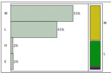
CPU usage related to this virtual environment is relatively in control, two ways to quickly
visualize this is to categorize each and color each CPU level which was done according
to Table 5.2 and then run a distribution of hostnames vs. CPU levels by hostname as
shown in Figure5.2.
Color CPU Level
0 MHz - 2333 MHz
2334 MHz - 4666 MHz
[image:41.596.227.399.310.398.2]4667 MHz - 7000 MHz ≥7001 MHZ
Table 5.2: Host CPU Level Color Legend
C PU R an g e (L /M /H /E) E H L M rtp -e sx -0 1 .c al o .c is co .c o m rtp -e sx -0 3 .c al o .c is co .c o m rtp -v n ap -0 1 .c al o .c is co .c o m rtp -v n ap -0 3 .c al o .c is co .c o m rtp -v n ap -0 5 .c al o .c is co .c o m rtp -v n ap -0 7 .c al o .c is co .c o m rtp -v n ap -0 9 .c al o .c is co .c o m rtp -v n ap -1 1 .c al o .c is co .c o m rtp -v n ap -1 3 .c al o .c is co .c o m rtp -v n ap -1 5 .c al o .c is co .c o m rtp -v n ap -1 7 .c al o .c is co .c o m rtp -v n ap -1 9 .c al o .c is co .c o m rtp -v n ap -2 1 .c al o .c is co .c o m rtp -v n ap -2 3 .c al o .c is co .c o m rtp -v n ap -2 5 .c al o .c is co .c o m rtp -v n ap -2 7 .c al o .c is co .c o m rtp -v n ap -2 9 .c al o .c is co .c o m rtp -v n ap -3 1 .c al o .c is co .c o m rtp -v n ap -3 3 .c al o .c is co .c o m rtp -v n ap -4 9 .c al o .c is co .c o m rtp -v n ap -5 1 .c al o .c is co .c o m rtp -v n ap -5 3 .c al o .c is co .c o m rtp -v n ap -5 5 .c al o .c is co .c o m Hostname Legend E H L M
Figure 5.2: Host CPU Usage by Host
As you can see from the figure that the environment is very well balanced with regards
to CPU usage. The hosts with a high number which were added to the environment at a
[image:41.596.173.460.436.670.2]shows another way to look at the distribution of CPU usage is to look at the percentage
that falls within each level.
[image:42.596.224.403.135.253.2]E H L M 2% 2% 41% 55% L M
Figure 5.3: Host CPU Usage Range
When looking at the statistics collected for the entire environment a few assumptions
can be made about the mean operational levels of the servers within the environment.
As shown in Table 5.1 it can be stated that on average the mean CPU usage in MHz
recorded is about the frequency of one CPU core per server in the environment. By
investigating server, not all servers are running at a similar level as shown in Figures
5.4(a)and 5.4(b).
3000 4000
CPU
Usage
(MHz)
07/04/2009 4:00:00 AM 07/08/2009 11:02:00 PM Timestamp
Mean Std N
Zero Mean ADF Single Mean ADF Trend ADF 3203.6767 243.14059 3384 -0.805608 -11.86121 -19.50525
Time Series CPU Usage (MHz) Hostname=rtp-vnap-03.calo.cisco.com
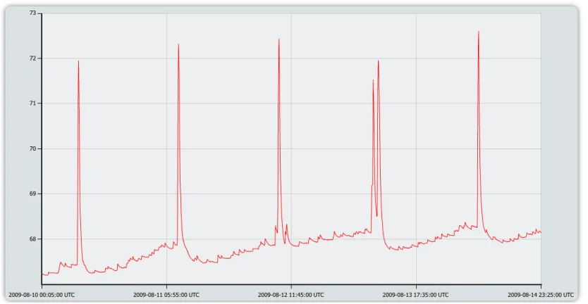
(a) rtp-vnap-03 80 90 100 110 120 130 140 150 160 CPU Usage (MHz)
07/04/2009 4:00:00 AM 07/08/2009 11:02:00 PM Timestamp
Mean Std N
Zero Mean ADF Single Mean ADF Trend ADF 89.937648 9.3793169 3384 -4.557258 -66.31962 -66.31364
Time Series CPU Usage (MHz) Hostname=rtp-vnap-53.calo.cisco.com
(b) rtp-vnap-53
Each of the servers above show a large difference in CPU usage this is due to the level of
activity of each VM running on the servers as well as the number of VMs actually running
on the server. Maybe setting a warning and critical threshold for each server could aid
in notifications of over-utilization of a single server and allow for load balancing.
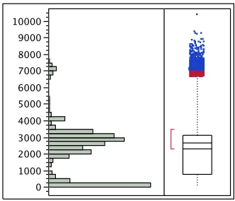
5.2.2 Memory Usage
Memory is the most important resource regarding the servers in a virtual environment.
There are technologies that VMware ESX leverages to conserve RAM within like VMs.
That being said, it is not predictable nor is it a replacement to physical memory. Looking
at Table 5.3 we can see that the mean memory usage, an average of 52 percent of the
RAM on each server is being consumed in this sample. Figure 5.5 does a great job
illustrating the memory usage within the virtual environment.
0 10 20 30 40 50 60 70 80 90
Figure 5.5: Memory Usage (%)
Statistic Memory (%)
Mean 52.062792
Std Dev 27.148344
Std Err Mean 0.0688247 Upper 95% Mean 52.197687 Lower 95% Mean 51.927897
N 155596
Quantile Memory (%)
100% (maximum) 88.03 75% (quartile) 71.54
50% (median) 66.41
25% (quartile) 26.04
[image:43.596.238.391.353.491.2]0% (minimum) 0
Table 5.3: Host Memory Counter Moments
Memory usage for this virtual environment while being stable is bi-modal. The
the environment is relatively stable there are two things to mention here. Most
impor-tantly there are some hosts which are heavily loaded and some hosts which have almost
no memory usage at all. Secondly if the hosts which have little or no memory usage
were to be removed from the dataset we would get a more accurate representation of
the data. Another way to view the data is memory usage for each host, this will provide
detailed information over time for each individual host. Figures5.6(a)and 5.6(b) both
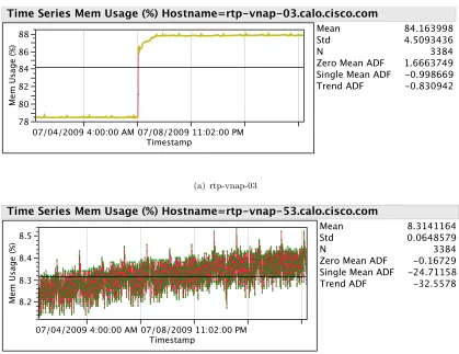
have two different stories attached to them.
78 80 82 84 86 88 Mem Us ag e (%)
07/04/2009 4:00:00 AM 07/08/2009 11:02:00 PM Timestamp
Mean Std N
Zero Mean ADF Single Mean ADF Trend ADF 84.163998 4.5093436 3384 1.6663749 -0.998669 -0.830942
Time Series Mem Usage (%) Hostname=rtp-vnap-03.calo.cisco.com
(a) rtp-vnap-03 8.2 8.3 8.4 8.5 Mem Us ag e (%)
07/04/2009 4:00:00 AM 07/08/2009 11:02:00 PM Timestamp
Mean Std N
Zero Mean ADF Single Mean ADF Trend ADF 8.3141164 0.0648579 3384 -0.16729 -24.71158 -32.5578 Time Series Mem Usage (%) Hostname=rtp-vnap-53.calo.cisco.com
[image:44.596.120.539.222.545.2](b) rtp-vnap-53
Figure 5.6: Host Memory Time Series
Take rtp-vnap-03 for example, the memory usage on this host is extremely high compared
to rtp-vnap-53. The reason for this is rtp-vnap-53 was added to the environment at a
much later date and does not have as many virtual machines associated with it.
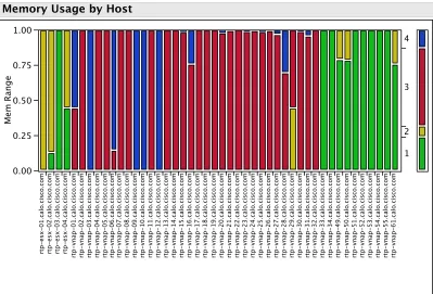
To provide a good overview of the entire virtual environments’ memory footprint of each
host, we can perform a bivariate analysis between memory levels defined in Table 5.4
identify hosts that a dangerous amount of memory being consumed and allow for relation
or re-assignment of these memory offending virtual machines.
Color Memory Percentage
0% - 24%
25% - 49%
50% - 74%
[image:45.596.231.401.140.228.2]75% - 100%
Table 5.4: Host Memory Level Color Legend
Mem Ran g e 0.00 0.25 0.50 0.75 1.00 rtp -e sx -0 1 .c al o .c is co .c o m rtp -e sx -0 2 .c al o .c is co .c o m rtp -e sx -0 3 .c al o .c is co .c o m rtp -e sx -0 4 .c al o .c is co .c o m rtp -v n ap -0 1 .c al o .c is co .c o m rtp -v n ap -0 2 .c al o .c is co .c o m rtp -v n ap -0 3 .c al o .c is co .c o m rtp -v n ap -0 4 .c al o .c is co .c o m rtp -v n ap -0 5 .c al o .c is co .c o m rtp -v n ap -0 6 .c al o .c is co .c o m rtp -v n ap -0 7 .c al o .c is co .c o m rtp -v n ap -0 8 .c al o .c is co .c o m rtp -v n ap -0 9 .c al o .c is co .c o m rtp -v n ap -1 0 .c al o .c is co .c o m rtp -v n ap -1 1 .c al o .c is co .c o m rtp -v n ap -1 2 .c al o .c is co .c o m rtp -v n ap -1 3 .c al o .c is co .c o m rtp -v n ap -1 4 .c al o .c is co .c o m rtp -v n ap -1 5 .c al o .c is co .c o m rtp -v n ap -1 6 .c al o .c is co .c o m rtp -v n ap -1 7 .c al o .c is co .c o m rtp -v n ap -1 8 .c al o .c is co .c o m rtp -v n ap -1 9 .c al o .c is co .c o m rtp -v n ap -2 0 .c al o .c is co .c o m rtp -v n ap -2 1 .c al o .c is co .c o m rtp -v n ap -2 2 .c al o .c is co .c o m rtp -v n ap -2 3 .c al o .c is co .c o m rtp -v n ap -2 4 .c al o .c is co .c o m rtp -v n ap -2 5 .c al o .c is co .c o m rtp -v n ap -2 6 .c al o .c is co .c o m rtp -v n ap -2 7 .c al o .c is co .c o m rtp -v n ap -2 8 .c al o .c is co .c o m rtp -v n ap -2 9 .c al o .c is co .c o m rtp -v n ap -3 0 .c al o .c is co .c o m rtp -v n ap -3 1 .c al o .c is co .c o m rtp -v n ap -3 2 .c al o .c is co .c o m rtp -v n ap -3 3 .c al o .c is co .c o m rtp -v n ap -3 4 .c al o .c is co .c o m rtp -v n ap -4 9 .c al o .c is co .c o m rtp -v n ap -5 0 .c al o .c is co .c o m rtp -v n ap -5 1 .c al o .c is co .c o m rtp -v n ap -5 2 .c al o .c is co .c o m rtp -v n ap -5 3 .c al o .c is co .c o m rtp -v n ap -5 4 .c al o .c is co .c o m rtp -v n ap -5 5 .c al o .c is co .c o m rtp -v n ap -6 1 .c al o .c is co .c o m Hostname 1 2 3 4
Memory Usage by Host
Figure 5.7: Overall Memory Usage
A solution to this unbalanced bi-modal server memory usage would be to provide an
automated migration of the virtual machines to a lightly loaded server as opposed to the
server with high memory usage. VMware provides this capability within a cluster, but
not between clusters. So for this environment running an analysis like the time series
charts in the figure above weekly would provide the information to the administrators
[image:45.596.121.520.265.536.2]5.2.3 Disk Usage
Disk usage when polled from each server can be quite diverse. There are times when
servers have most of their VMs shutdown, during these times the disk usage will be 0.
There are also times when a large portion of the VMs running on that host are powered
on and start thrashing the storage array, this can be seen when looking at the quantile
statistics in Table 5.5and the distribution of the data in Figure5.8.
[image:46.596.231.397.240.380.2]0 10000 20000 30000 40000 50000 60000 70000 80000 90000 100000 110000 120000 130000
Figure 5.8: Disk Usage (KB/sec)
Statistic Disk (KB/sec)
Mean 1137.1612
Std Dev 2652.9798
Std Err Mean 6.7256573 Upper 95% Mean 1150.3433 Lower 95% Mean 1123.979
N 155596
Quantile Disk (KB/sec)
100% (maximum) 128007 75% (quartile) 1185
50% (median) 818
25% (quartile) 271
0% (minimum) 0
Table 5.5: Host Disk Counter Moments
While the disk usage data is an important factor within the environment, due to its
arbitrary context on the servers its usefulness should be questioned. In this environment
all of the virtual machines are running off the storage array so any number for disk
usage on the servers is going to be duplicated on the storage array as well. There is
not a correlation with disk usage and cpu usage or memory usage. The web application
monitoring of disk usage should be sufficient in the analysis of disk usage.
An interesting observation about disk usage is the variability shown in Figure 5.8 and
very wild data source. Take for instance if a virtual machine is patching or booting
up/shutting down, the disk usage will spike. The quantile statistics prove that 75% of
the data falls right around the mean with a value of 1185 but has a maximum of 128007.
The lack of correlation between is also evident by looking at Figure5.9. You can see by
the disk usage levels that do not coincide with the CPU or Memory levels.
5.2.4 Counter Overview
A quick look at the counter vs. timestamp graph in Figure 5.9 will show each data
source split by CPU usage levels demarcated by the levels defined in Table 5.2. This
chart does a fantastic job at detailing what the other counters are polled at when CPU
is a specific level. On top of that it also shows a simple time series of the three counters
for all the hosts in one view.
CPU
Usage
(MHz)
Mem
Us
ag
e (%)
Di
sk
U
sa
g
e
(K
B/
s)
0 2000 4000 6000
20 30 40 50 60 70
0 5000 10000 15000 20000
07/01/2009 12:00:00 AM 07/03/2009 12:00:00 AM 07/05/2009 12:00:00 AM 07/07/2009 12:00:00 AM 07/09/2009 12:00:00 AM 07/11/2009 12:00:00 AM 07/13/2009 12:00:00 AM Timestamp
Legend
E H
L M
[image:47.596.115.522.347.688.2]Counters vs. Timestamp by CPU Level
5.2.5 Host Data Source Correlations
It is always important to find relationships between any of the variables within a system.
A multivariate scatterplot matrix shown in Figure5.10 was used to determine if any of
the variables collected for the servers were correlated in any way. Each of the plots
show a large amount of variability in the response thus making it difficult to draw any
conclusions from this chart. The r value at 0.6496 tells us there is a positive relationship
between memory usage and CPU usage.
0 2000 4000 6000 8000
0 10 20 30 40 50 60 70 80
0 20000 40000 60000 80000 100000 120000
CPU Usage (MHz)
r=0.6496
r=0.3103
0 2000 5000 8000
r=0.6496
Mem Usage (%)
r=0.0661
0 20 40 60 80
r=0.3103
r=0.0661
Disk Usage (KB/s)
0 30000 70000
[image:48.596.119.524.249.644.2]Scatterplot Matrix
5.3 Storage Analysis
High performance shared storage is required in a virtual environment if certain
virtu-alization technologies are implemented. For example to provide high availability and
dynamic load balancing between servers within a cluster, shared storage is required.
That being said, the performance of the shared storage is crucial to the environments
overall health and performance. Initially the storage array had a daunting amount of
variables that were polled, 123 to be exact. Most of these 123 values are collected for
each object within the array. It would be impossible to monitor all 123 values for every
object on a regular basis.
The web application only polled information on the service processors and used that
as an overall performance metric. While this performs its task well, it is hard to know
everything about the storage environment just by analyzing the service processors. There
are many more types of objects that have similar data relating to the objects respectively.
The objects that makeup a storage array are defined in Table 5.6. For example there
could be a low load on the service processor all coming from one LUN with a LUN
utilization in the 80% range or higher. The VMs running on that LUN will be performing
unacceptably slow while the rest of the environment would be performing just fine. In
order to determine the performance each LUN would need to be analyzed. To effectively
perform the analysis on every LUN the number of counters that are polled must be
reduced.
Object Name Quantity
Service Processors 2
LUN 34
Disk 105
Raid Group 17
[image:49.596.235.399.516.602.2]Port 8
Table 5.6: Storage Array Objects
The service processors of the storage array are the active/active redundant portions
which control are I/O between the backend (drives) and the hosts in the virtual
envi-ronment. Below are some stats collected on determinant factors of performance in a
10 20 30 40 50
(a) Utilization (%)
0 20 40 60 80 100 120 140 160 180
(b) Queue Length
0 10 20 30 40 50 60 70 80 90
(c) Response Time (ms)
1000 2000 3000 4000 5000 6000 7000
[image:50.596.159.471.101.513.2](d) Throughput (IOPS)
Figure 5.11: Service Processor Distributions
5.3.1 Utilization
Utilization is a good metric to see an overview of the storage arrays’ workload, it is not
a great metric to understand actual usage. Be that as it may, it is a good way to see
if there are any contention points within the service processors that must be addressed.
According to the data in Table5.7mean utilization is at an acceptable level. Even when
SP A
Statistic Utilization (%)
Mean 14.75772
Std Dev 3.0561869
Std Err Mean 0.0328035 Upper 95% Mean 14.822022 Lower 95% Mean 14.693417
N 8680
SP B
Statistic Utilization (%)
Mean 13.0711
Std Dev 3.1295512
Std Err Mean 0.0335909 Upper 95% Mean 13.136946 Lower 95% Mean 13.005254
N 8680
Table 5.7: SP A/B Array Utilization Moments
SP A
Quantile Utilization (%)
100% (maximum) 54.7093 75% (quartile) 14.876 50% (median) 14.0625 25% (quartile) 13.5225 0% (minimum) 10.8731
SP B
Quantile Utilization (%)
100% (maximum) 53.3225 75% (quartile) 13.0363 50% (median) 12.4189 25% (quartile) 11.9736 0% (minimum) 10.3333
Table 5.8: SP A/B Array Utilization Quantiles
5.3.2 Queue Length
Queue length is the number of transactions that are waiting on the service processor, as
the queue length increases the potential performance of the array will decrease. On this
storage array the majority of the time the queue length is at a reasonable level. When
looking at the quartiles in Table 5.10 it is evident that at times the queue size spikes
very high. The large queue here can cause a potentially crippling performance deficit
on the storage array.
SP A
Statistic Queue Length
Mean 2.2106611
Std Dev 10.035682
Std Err Mean 0.1077177 Upper 95% Mean 2.4218133 Lower 95% Mean 1.9995088
N 8680
SP B
Statistic Queue Length
Mean 1.4223081
Std Dev 7.5786827
Std Err Mean 0.0813456 Upper 95% Mean 1.5817647 Lower 95%