Tutorial in biostatistics: sample sizes for parallel group clinical trials with binary data

(1)

This is a repository copy of Tutorial in biostatistics: sample sizes for parallel group clinical trials with binary data.

White Rose Research Online URL for this paper: http://eprints.whiterose.ac.uk/145472/

Version: Accepted Version Article:

Julious, S.A. and Campbell, M.J. orcid.org/0000-0003-3529-2739 (2012) Tutorial in biostatistics: sample sizes for parallel group clinical trials with binary data. Statistics in Medicine , 31 (24). pp. 2904-2936. ISSN 0277-6715

https://doi.org/10.1002/sim.5381

This is the peer reviewed version of the following article: Julious, S.A. and Campbell, M.J. (2012) Tutorial in biostatistics: sample sizes for parallel group clinical trials with binary data. Statistics in Medicine , 31 (24). pp. 2904-2936, which has been published in final form at https://doi.org/10.1002/sim.5381. This article may be used for non-commercial purposes in accordance with Wiley Terms and Conditions for Use of Self-Archived Versions.

[email protected] https://eprints.whiterose.ac.uk/

Reuse

Items deposited in White Rose Research Online are protected by copyright, with all rights reserved unless indicated otherwise. They may be downloaded and/or printed for private study, or other acts as permitted by national copyright laws. The publisher or other rights holders may allow further reproduction and re-use of the full text version. This is indicated by the licence information on the White Rose Research Online record for the item.

Takedown

If you consider content in White Rose Research Online to be in breach of UK law, please notify us by

(2)

Tutorial in Biostatistics: Sample sizes for Parallel Group Clinical

Trials with Binary Data

Steven A. Julious and Michael J. Campbell

University of Sheffield

Correspondence to

(3)

SUMMARY

This article gives an overview of sample size calculations for a single response and a comparison of

two responses in a parallel group trial where the outcome is binary. Sample size derivation is given for trials where the objective is to demonstrate: superiority, equivalence, non-inferiority and

estimation to a given precision. For each type of trial the null and alternative hypotheses are described as well as how the impact these have on the sample size calculations. For each type of trial the calculations are highlighted through worked examples. Sample size tables for the different types of

trials and worked examples are given to assist in future calculations.

Key Words

(4)

An essential step in planning a trial is the calculation of a sample size which will give the minimum numbers required to meet the objectives of the study. We have already given a tutorial for the case where the endpoint is anticipated to have a Normal distribution [1]. This paper extends this work to discuss the situation where the primary endpoint is binary. A review of sample size formulas for the comparison of proportions has been published before [2]; this paper expands and updates that review.

Having as good an estimate as possible of the required sample size is important as studies that are either too small or too large may be judged unethical [5]. For example, a study that is too large could have met the objectives of the trial before the actual study end had been reached, and so some patients may have unnecessarily entered the trial and have been randomised to a therapy that can already be proven to be suboptimal. Conversely a trial that is too small may have little chance of meeting the study objectives, and patients may be entering a trial for no tangible benefit. The general approach to choosing sample size will be described in this article where the primary endpoint can be assumed to be binary and an estimate of the treatment response on at least one of the arms is available. The sections of the paper detail computation of sample sizes appropriate for:

1. Superiority trials.

2. Equivalence trials.

3. Non-inferiority trials. 4. As good as or better trials.

5. Trials to a given precision.

As in our earlier paper [1] a distinction is drawn between trials designed to demonstrate 'superiority' and trials designed to demonstrate 'equivalence' or 'non-inferiority'. We emphasise how differences in the null hypothesis can impact on calculations as well as in the estimation of the treatment response under the null and alternative hypothesis [3]. The ICH guidelines E3 and E9 provide general guidance on selecting the sample size for a clinical trial [6,7].

Using worked examples, we will also give a brief description of how the calculations can be undertaken in two popular packages PASS 11 [8] and nQuery 7 [9].

(7)

are given which do not require the use of tables for calculations. We assume that the reader is familiar with the concepts of Type I and Type II errors (and power) as discussed in an earlier tutorial article [1] and numerous books including [3-4].

2. SINGLE PROPORTION

In studies with a single binary response π_A there are two types of hypothesis that can investigated depending on whether the objective of the trial is to show the response is greater than or less than some hypothesised value - as in the null (Ho ) and alternative

(H1) hypothesis below

H0: The treatment has an effect in terms of the absolute risk being less or equal than

some pre-specified value (π_A ≤π_H).

H1: The treatment has an effect in terms of the absolute risk being greater than some

pre-specified value (π_A >π_H).

Alternatively

H0: The two treatments have equal effect with respect to the absolute risk difference (

H

A π

π = ).

H1: The two treatments are different with respect to the absolute risk difference (

H

A π

π ≠ ).

Even if we have a two (or more) arm trial we may still wish to investigate an hypothesis for a single arm. For example the primary endpoint may be clinical based on a continuous scale but we may wish also to show that for a particular adverse event the proportion of events on the investigative treatment arm π_A can be proved (at a given level of significance) to be less than some a priori set clinically important absolute risk i.e. π_A ≤π_H.

(8)

2.1. Confidence Interval Calculation

It is worth considering the calculation of confidence intervals for a single binary response before describing the sample size calculations. There are number of ways of a calculating a confidence interval [13]. Here we will concentrate on just two: the Normal approximation approach and the exact method. The Normal approximation is the most common approach for calculating confidence intervals. However, for rare events the Normal approximation may not hold and exact methods should be applied instead.

2.1.1. Normal Approximation

Under the Normal approximation the confidence interval for a single proportion is defined as

(1) p±Z1−α2se(p),

where p is the estimated response from the trial, se(p)= p(1− p) n, Z₁₋_α_/₂ the

)

(

1−α/2 % point of the standard Normal distribution

and α the level of statistical significance (α=0.05 would give 95% confidence intervals). This method is referred to as the Wald method [13].

2.1.2. Exact Confidence Intervals

The confidence interval calculations described as "exact" confidence intervals are also known as Clopper-Pearson confidence intervals [14]. These confidence intervals are calculated by summing each of the tail probabilities from the binomial distribution, given the observed number of cases (k) for the sample size (n). Therefore, defining the individual cell probabilities as

(2) Pr( ) pk(1 p)(n k) k

n k

X _ − −

     =

= ,

the lower limit of the confidence interval is calculated as the largest value of p such that the lower tail area of the cumulative distribution is no more than α/2. Likewise the upper limit is calculated as the smallest point where the cumulative distribution equals or exceeds 1-α/2. Formally, the lower point of a confidence interval is defined as the maximum value pL such that

(3) _ (1− )( ) ≤α/2 

  

 −

=

∑

n i

L i

L k

p p i n

(9)

whilst the upper point is defined as the minimum value pU such that,

(4) (1 )( ) 1 /2

0

α − ≥ −

    

 −

=

∑

n i

U i

U k

i

p p

i n

.

An alternative approach to calculate exact confidence intervals would be to use the link between binomial and beta distributions [15-16]. From this the lower bound is defined as

(5) p_L =1−BETAINV

(

1−α 2,n−k+1,k

)

,

and upper as

(6) p_U =BETAINV

(

1−α 2,k+1,n−k

)

.

Here, α is the level of statistical significance (α =0.05 would give 95% confidence intervals), k the number of events observed n the sample size on the investigative treatment arm and BETAINV

( )

• refers to the cumulative distribution function of a Beta distribution. The upper and lower bounds calculated from (5) and (6) will provide range of plausible values that the population proportion is likely to be within. The theoretical rationale behind using the Beta distribution is more complicated than for standard Normal approximation calculations. However, operationally they are easy to calculate and can be calculated in most statistical packages. The BETAINV

( )

• notation given in this paper is taken from the computer package SAS.

Identical confidence intervals can also be obtained using the link between the F distribution and the binomial distribution although with a more complicated nomenclature [13,15,16]. This link will not be discussed further.

2.2. One Tailed or Two Tailed?

The question of whether to calculate one or two tailed confidence intervals is not straightforward [17]. It depends on whether we wish to provide an estimate of the plausible range for the true value (two tailed) or a value which you are confident will not be exceeded by the true value (one tailed).

For rare events we are often interested in a one tailed confidence interval such that a (upper) one-tailed (1-α %) bound is estimated from

(7) BETAINV

(

1−α,k+1,n−k

)

(10)

The emphasis in this paper, however, will be on two tailed confidence interval estimation i.e. using (5) and (6). As we are only interested in one tail of the 95% confidence interval this would be equivalent to a one tailed confidence interval but with α set at 2.5%.

2.3. Sample Size Calculation

To calculate the sample size for an anticipated response π_A which we wish to assess as being less than (or greater) then a hypothesised value π_H the following Normal approximation result could be used [18]

(8)

[

]

(

)

2

2 2

/ 1

-1 (1 ) Z (1 )

Z H A H H A A n π π π π π π _α β − − + − = − .

This sample size calculation would be consistent with a Normal approximation being used for the confidence interval. Here, andβ are the overall Type I and Type II errors level.

An alternative equation is

(9)

[

]

(

)

2

2 2 / 1 -1 Z Z ) 1 ( H A n π π π

π _β _α

− + −

= −

.

where π =(π_A +π_H)/2. Equation (9) gives similar answers to equation (8) for π_A <π_H but gives a slightly larger sample size for π_A >π_H.

(11)

Table 1. Sample size calculations for a one arm trial for a single binary response using the Normal approximation for 90% power and a 95% confidence interval for an alternative hypothesis of π_A >π_H using (8).

H π

A

π _0.05 _0.10 _0.15 _0.20 _0.25 _0.30 _0.35 _0.40 _0.45 _0.50 _0.55 _0.60 _0.65 _0.70 _0.75 _0.80 _0.85 _0.90

0.10 264 0.15 79 438 0.20 40 122 589 0.25 25 59 158 718 0.30 17 35 74 189 825 0.35 12 24 43 87 214 912 0.40 10 17 29 50 97 233 977 0.45 8 13 20 33 56 105 248 1022 0.50 6 10 15 23 36 60 111 257 1045 0.55 5 8 12 17 25 38 62 114 261 1047 0.60 4 6 9 13 18 26 40 64 115 259 1028

0.65 3 5 7 10 14 19 27 40 63 113 252 988

0.70 3 4 6 8 11 14 19 27 40 62 109 240 927

0.75 2 4 5 6 8 11 14 19 27 38 59 103 222 845

0.80 2 3 4 5 7 8 11 14 19 25 36 55 94 200 742

0.85 2 2 3 4 5 7 8 10 13 17 23 33 49 82 171 617

0.90 1 2 3 3 4 5 6 8 10 12 16 21 28 42 68 137 471

0.95 1 2 2 3 3 4 5 6 7 8 10 13 17 23 32 51 96 301

Using a binomial distribution an estimate of the power can be obtained from equations (10) and (11) [19]

(10) A N j

j A q j j n ₋ = −      

∑

(1 )

0

π π

where q is the largest integer of k such that

(11) _π −π ≤α

     − =

∑

N j

H j H k j j n ) 1 ( 0

Table 2 gives the sample sizes estimate from (10) and (11). As with Table 1 for π_A<

H

π _replaceπ_A_by1−π_A_andπ_H_by1−π_H_{. It should be noted that here}π_A >π_H

and πA<πH_{do not quite give symmetric results. There were seven instances where}

the sample size calculated for πA>πH_{was slightly higher than the sample size}

estimates “equivalent” for πA<πH_{. These are shown (with the sample size for}πA H

π

(12)

Table 2. Sample size calculations for a one arm trial for a single binary response using a binomial distribution for 90% power and a two sided significance level of 5% for an alternative hypothesis of π_A >π_H using equation (10) and (11) Superscript entries are shown when A and H are swapped and the results differ.

H π

A

π 0.05 0.10 0.15 0.20 0.25 0.30 0.35 0.40 0.45 0.50 0.55 0.60 0.65 0.70 0.75 0.80 0.85 0.90 0.10 316

0.15 102 492 0.20 55 149 641 0.25 38 75 183 768 0.30 27 49 90 212 870 0.35 18 34 56 103 237 949 0.40 16 23 39 60 112 255 1021 0.45 14 20 26 42 66 116 266 1066 0.50 12 15 20 30 42 70 121 274 1080 0.55 8 13 16 22 31 44 71 125 273 1082 0.60 7 10 14 18 22 32 46 72 121 275 1059 0.65 6 9 11 13 18 24 33 47 69 124 265 1017

0.70 6 8 10 11 15 18 23 30 46 68 117 252 950

0.75 5 7 9 9 12 13 17 23 32 44 64 111 231 863

0.80 5 5 6 8 9 11 14 17 21 31 39 59 99 207 764

0.85 5 5 6 6 7 8 10 11 15 19 27 36 55 87 180 632

0.90 5 5 5 5 6 8 9 9 13 14 19 21 32 45 73 143 484

0.95 5 5 5 5 5 5 7 7 8 9 10 15 18 25 35 51 100 301

Comparing Table 1 with the equivalent values in Table 2 we can see that equation 8) estimates the sample size to be smaller than equations (10) and (11). This difference in the sample size is due to two reasons. Firstly, Fisher’s Exact tests is more conservative than the asymptotic test and so requires a large sample size for a given significance level and power. Secondly, because of the discrete nature of the binomial distribution it may be impossible to get an exact type I and Type II error. One can easily find the actual significance level and power, for a given sample size, that a binomial distribution produces. If these actual values are inserted into (9) we would find results comparable to Tables 1 and 2

For completeness we include the following result which gives the sample size where an arcsine transformation (if y=sin(x) then x=arcsin(y)) is applied to the hypothesised and anticipated responses [20]. The sample sizes estimated from this result are comparable to earlier results and will not be discussed further.

(12)

[

]

(

)

2

2 2 / 1 -1

) arcsin( )

arcsin( 4

Z Z

H A

n

π π

α β

− +

= −

(13)

2.3.1. Worked Example 1 – Sample Size Calculation for a Single Binary Response

An investigator is designing a placebo controlled trial to investigate a new treatment in depression. The sample size for the primary endpoint was calculated to be 525 patients per arm. From experience with other compounds for the same indication the adverse event rate is anticipated to be around 50% in the trial population The compound under investigation is expected to have a lower adverse event rate of around 40% and the investigator wishes to demonstrate using a 95% confidence interval (equivalent to a Type I error of 2.5%) and 90% power that the event rate is less than 50%.

Since A < H we look up 1- A and 1- H and using the Normal approximation result

given by equation (8) the required sample size from Table 1 for H=0.5 and A=0.6 is

estimated to be 259 patients. Alternatively using the binomial approach, and results (10) and (11), Table 2 estimates the sample size to be 275 patients. As the sample size is less than the sample size of 525 patients being recruited the investigator has sufficient power for the additional objective.

In repeating the calculation in PASS we believe there may be an error in the way PASS estimates sample size for one binomial proportion. To estimate the sample size on PASS you select the menu options Proportions /One Proportion / Test (Inequality) and then the icon Test for One Proportion (Proportions). For this problem, the Alternative Hypothesis dialogue can be set to ‘p<p0’ and the Type I error as 0.025. PASS can either estimate the sample size (for a given power) or the power (for a given sample size). PASS estimates the sample size to be 263 patients

(14)

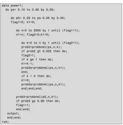
Figure 1. Example SAS code for calculating sample sizes using a binomial distribution for the alternative hypothesis of π_A >π_H.

data power1;

do ps= 0.10 to 0.95 by 0.05;

do p0= 0.05 to ps-0.05 by 0.05; flag1=0; k1=0;

do n=3 to 2000 by 1 until (flag1=1); n1=n; flag2=0;k1=0;

do k=0 to n by 1 until (flag2=1); prob2=probbnml(ps,n,k);

if prob2 gt 0.025 then do; flag2=1;

if k ge 1 then do; k1=k-1;

prob2a=probbnml(ps,n,k1); end;

if k = 0 then do; k1=0;

prob2a=probbnml(ps,n,k1); end;end;end;

prob3=probbnml(p0,n,k1); if prob3 ge 0.90 then do; flag1=1;

end;end; output; end;end; run;

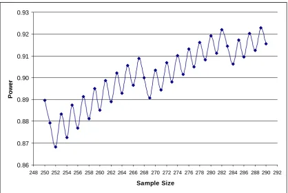
There is an interesting issue with this programming approach. Figure 2 gives the power for the study for different sample sizes ranging from 250 to 290 patients for the worked example of π_A=0.40 and π_H=0.50. We can see from Figure 2 how a power of 90% is obtained for a sample size of 263 patients but now we have less than 90% power for 264 patients!. In fact it is not until the sample size is 275 that for both this and the subsequent sample sizes does power exceed 90%. The sample size of 275 patients is what is given in Table 2 and by Equations 10 and 11.

[image:14.595.90.508.107.529.2]

(15)

[image:15.595.94.513.191.471.2]

stop for given integer sample size if it, and sample sizes up to 10 greater, all had greater than 90% power. Figure 3 gives example SAS code for this calculation.

Figure 2. Power for a given sample size for the case π_A=0.40 and π_H=0.50 where we wish to show that π_A <π_H with a two-sided 95% confidence interval.

0.86 0.87 0.88 0.89 0.90 0.91 0.92 0.93

248 250 252 254 256 258 260 262 264 266 268 270 272 274 276 278 280 282 284 286 288 290 292

Sample Size

P

o

w

(16)

[image:16.595.92.507.107.653.2]

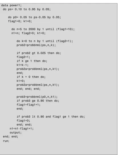
Figure 3. SAS code used to generate Table 2 for calculating sample sizes using a binomial distribution for the alternative hypothesis of π_A >π_H.

data power1;

do ps= 0.10 to 0.95 by 0.05;

do p0= 0.05 to ps-0.05 by 0.05; flag1=0; k1=0;

do n=5 to 2000 by 1 until (flag1=10); n1=n; flag2=0; k1=0;

do k=0 to n by 1 until (flag2=1); prob2=probbnml(ps,n,k);

if prob2 gt 0.025 then do; flag2=1;

if k ge 1 then do; k1=k-1;

prob2a=probbnml(ps,n,k1); end;

if k = 0 then do; k1=0;

prob2a=probbnml(ps,n,k1); end; end; end;

prob3=probbnml(p0,n,k1); if prob3 ge 0.90 then do; flag1=flag1+1;

end;

if prob3 lt 0.90 and flag1 ge 1 then do; flag1=0;

end; end; n1=n1-flag1+1; output;

end; end; run;

(17)

PASS also has two other methods giving sample size estimates for two Normal approximation approaches (both with and without a continuity correction). Both approaches are a little different from (9) (and indeed (8)) in that the variance estimate of the treatment effect (under the null or alternative hypothesis) either uses just π_A or

H

π and not both (as in (9) and (8)). For the calculation of the result that uses π_A (termed p hat in PASS) the sample size is estimated to be 251 patients.

In nQuery to estimate the sample size equivalent to the exact approach given in equations (10) and (11) the options Proportions /One /Exact test for a single proportion need to be selected. nQuery does not give the sample size directly but the power for a given sample size. To save doing many iterations, equation (9) could be used for an initial sample size. nQuery only gives power to 2 decimal places in the calculations spreadsheet (actually returns as a percentage equivalent to two decimal places) with more significant digits appear at the bottom of the window. For the spreadsheet the power is always rounded down. Hence, a power of 89.99 will appear as 89% in the output. nQuery gives a sample size of 274 patients.

(18)

2.4. Sample Size Calculation Re-visited – Sample Size Based on Feasibility

2.4.1. Precision Based Approach

As highlighted in Worked Example 1, in clinical trials the primary objective is usually not to estimate a single absolute risk but rather compare an investigative treatment with a control for a given objective and endpoint. The sample size would therefore be estimated from the primary endpoint and hence ‘fixed’ with respect to the objective for the single absolute risk. In this context therefore the objective may not be to prove a risk is less than some bound but to quantify the likely range of values that the risk could plausibly be – through a confidence interval.

In Section 3.5 precision based trials are described where the objective is to quantify the risk difference against control.

For a single risk the precision of the trial can be estimated from

(13)

n p p Z

w= 1−α2 (1− ),

where w here is defined as half the width for a confidence interval. Here, it is assumed that both n and p are known. To estimate a sample size to have a required precision, w, about p then the following result could be used.

(14) ₂

2 2 /

1 (1 )

w p p Z

n= −α − .

If exact confidence intervals are being used then we can estimate the precision for a trial from

(15) w=

(

BETAINV

(

1−α 2,k+1,n−k

)

+BETAINV

(

1−α 2,n−k+1,k

)

−1

)

/2

where k is estimated from k=pn. To estimate the sample size we can iterate on n until we get a sample size with the requisite precision for a given p.

2.4.2. Probability of Seeing an Event

(19)

Hence, if the risk for a particular adverse event is p then the probability that k or more adverse events will be observed with n subjects can be calculated from

(16)

∑

(

)

−

=

−

−       −

= 1

0

1 1

k

x

x n x

k p p

x n p

2.4.2.1. Worked Example 2 – Calculating a Probability of Observing an Adverse Event

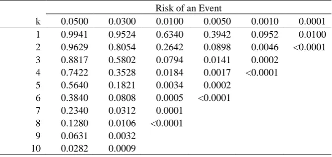
A Phase II trial has been designed where the number of patients per arm is 100. For the investigative treatment a number of adverse events are being monitored with difference anticipated risks. Table 3 gives the probability of observing various numbers of adverse events for different anticipated population risks.

[image:19.595.97.432.425.583.2]

From Table 3 we can see that for a risk of an adverse event of 1/1000 we would have less than 10% chance of observing at least one adverse event. Also for a risk of 1/10,000 we’d have only a 1% chance of seeing at least one adverse event.

Table 3. Probablilities of observing a given number of adverse events or more (k) for given anticipated risks for a sample size of 100 patients.

Risk of an Event

k 0.0500 0.0300 0.0100 0.0050 0.0010 0.0001

1 0.9941 0.9524 0.6340 0.3942 0.0952 0.0100

2 0.9629 0.8054 0.2642 0.0898 0.0046 <0.0001

3 0.8817 0.5802 0.0794 0.0141 0.0002

4 0.7422 0.3528 0.0184 0.0017 <0.0001

5 0.5640 0.1821 0.0034 0.0002

6 0.3840 0.0808 0.0005 <0.0001

7 0.2340 0.0312 0.0001

8 0.1280 0.0106 <0.0001

9 0.0631 0.0032

10 0.0282 0.0009

We recommend that a table such as Table 3 be calculated for all planned clinical trials.

If no adverse events are observed the results in Table 3 could be used to put the results into some context. This could be done in context also with the ‘3 over n’ (3/n) rule [12]. The 3/n rule gives the approximate upper tail of a one-sided 95% confidence interval when zero events are observed and is derived using the Poisson approximation to from equation 16).

(20)

event we anticipated the population risk to be 1/2000=0/005 and thus that a priori we would anticipate that there was a probability of 0.39 of observing at least one adverse event. We could highlight this probability when discussing the result. Also, we could state that, based on the observed trial data, we can rule out a risk of 3/100 (3/n)=0.03 or 3% or greater.

3. PARALLEL GROUP TRIALS

3.1. Superiority Trials

With a superiority trial the objective is to determine whether there is evidence of a statistical difference in the comparison of interest between the regimens with reference to the null hypothesis that the regimens are the same. The null (H0) and alternative

(H1) hypotheses may take the form:

Ho: The two treatments are not different (π_A =π_B).

H1: The two treatments are different (π_A ≠π_B) i.e. either A is superior to B or B is

superior to A.

For a two-sided superiority trial there are two chances of rejecting the null hypothesis and thus making a Type I error. The null hypothesis can be rejected if p_A > p_B or if

B

A p

p < by a statistically significant amount. As there are two chances of rejecting the null hypothesis the statistical test is referred to as a two tailed test with each tail allocated an equal amount of the Type I error (of 2.5%). The sum of these tails adds up to the overall Type I error rate of 5%. Thus, the null hypothesis can be rejected if the test of π_A >π_B is statistically significant at the 2.5% level of significance or the test of π_A <π_B is statistically significant at the 2.5% level.

The purpose of the sample size calculation is hence to provide sufficient power to reject Ho when in fact some alternative hypothesis is true

3.1.1. Summarising Clinical Trials with Binary Data

(21)

Table 4. Summary table for a clinical trial with a binary outcome

Outcome

Treatment 1 0 Sample Size

A p_A 1− p_A n_A

B p_B 1− p_B n_B

Overall Response p=(nApA+nBpB)/(nA 1− p

B

A n

n

n= +

The absolute risk reduction is probably the simplest way of summarising binary data which is p_A − p_B_{, and this is the scale that we will focus on.}

One drawback of working with the absolute risk difference is that it is bounded by (-1, 1). This bounding can adversely affect inference – especially when both responses are near one of the bounds.

3.1.2. Sample Sizes for a Superiority Trial

For the special case of equally sized arms in the trial the sample size is

(17)

(

)

(

)

2

2 1

2

1 2 (1 ) (1 ) (1 )

B A B B A A A Z Z n π π π π π π π π _β α − − + − + − = − −

(where π =(πA +πB)/2₎

Since the expressions under the square roots are relatively stable to changes in the ’s, this is often simplified to [3,27,28]

(18)

[

]

(

)

(

)

2

2 2 / 1

-1 Z (1 ) (1 )

Z B A B B A A A n π π π π π π α β − − + − + = − .

The result (18) gives the maximum sample size for the case where π =0.5 [3]. From this fact and within this range for the average response a quick estimate of the sample size, for 90% power and two-sided significance level of 5%, can be obtained from the following result [3]

(19)

(

)

2

25 . 5 B A A n π π − = .

(22)

(20)

(

)

2

4 B A A n π π − = .

Both of these results will provide conservative “maximum” estimates of the sample size.

For these sample size calculations we have assumed equal allocation to treatment. For fixed allocation to treatment there are extensions to these results [28] and for random allocation there are alternative results [29]. In addition we have assumed there will be just a single endpoint in the trial. For calculations with multiple endpoints there are alternative calculations [30-32].

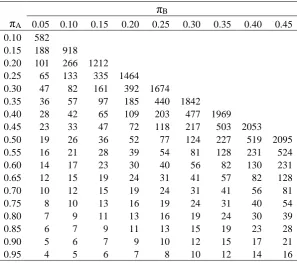
[image:22.595.97.395.368.631.2]

Sample sizes for selected values of Aand B using equation (17) are given in Table 5

Table 5. Sample size estimates using result (17) for one arm of a parallel group trial for various expected outcome responses for a given treatment ( A) and

comparator ( B) for a two sided type I error rate of 5% and 90% power

B

A 0.05 0.10 0.15 0.20 0.25 0.30 0.35 0.40 0.45

0.10 582 0.15 188 918 0.20 101 266 1212

0.25 65 133 335 1464

0.30 47 82 161 392 1674

0.35 36 57 97 185 440 1842

0.40 28 42 65 109 203 477 1969

0.45 23 33 47 72 118 217 503 2053

0.50 19 26 36 52 77 124 227 519 2095

0.55 16 21 28 39 54 81 128 231 524

0.60 14 17 23 30 40 56 82 130 231

0.65 12 15 19 24 31 41 57 82 128

0.70 10 12 15 19 24 31 41 56 81

0.75 8 10 13 16 19 24 31 40 54

0.80 7 9 11 13 16 19 24 30 39

0.85 6 7 9 11 13 15 19 23 28

0.90 5 6 7 9 10 12 15 17 21

0.95 4 5 6 7 8 10 12 14 16

If we intend to use a continuity corrected chi-squared test in the analysis then (17) and (18) could be used to estimate initial values of the sample size which are then increased to account for the conservative nature of this test using the following result [28].

(21) 2 ) ( 4 1 1

4 __

(23)

[image:23.595.97.471.215.485.2]

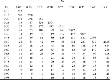
Table 6 gives estimates of the sample size using equations (21) with (17)

Table 6. Sample size estimates using result (17)) with a continuity correction for one arm of a parallel group trial for various expected outcome responses for a given treatment ( A) and comparator ( B) for a two sided type I error rate of 5%

and 90% power

B

A 0.05 0.10 0.15 0.20 0.25 0.30 0.35 0.40 0.45

0.10 622

0.15 208 958

0.20 114 286 1252

0.25 75 147 355 1504

0.30 55 92 175 412 1714

0.35 43 65 107 199 460 1882

0.40 34 49 73 119 217 497 2009

0.45 28 39 54 80 128 231 523 2093

0.50 24 31 42 59 85 134 241 539 2135

0.55 20 26 33 45 61 89 138 245 544

0.60 18 21 28 35 46 63 90 140 245

0.65 16 19 23 29 36 47 64 90 138

0.70 13 16 19 23 29 36 47 63 89

0.75 11 13 17 20 23 29 36 46 61

0.80 10 12 14 17 20 23 29 35 45

0.85 9 10 12 14 17 19 23 28 33

0.90 8 9 10 12 13 16 19 21 26

0.95 7 8 9 10 11 13 16 18 20

If the final analysis is to be a Fisher’s Exact test then the sample size calculation is not so straightforward. The sample size is calculated in two stages. Conditional on the number of events observed k in _A n subjects on treatment A and _A k events in _B n _B subjects on treatment B such that k =k_A +k_B_and n=n_A +n_B, we can use a hypergeometric distribution to find the probability of a number of events ki<nA as

(22) ( | , , ) .

            −       = = k n k k n k n n n k k P P i B i A A i k_i

(24)

(23) ( | , , ) . 0

∑

=             −       = A i k k i B i A A A k n k k n k n n k n k F

For the subset of tables where we reject the null hypothesis from (22) we can estimate the power under the alternative hypothesis, in equation (24).

(24) A

(

1

)

A A B

(

1

)

nBkB .

B k B k n A k A B B A A k n k n

Power − − −

           

=

∑∑

_π _π − _π _π

Thus for a given k , _A k , _B n and _A n we can estimate the power. Hence, through _B iteration we can estimate the sample size for a given π_A and π_B for a given nominal power. As for a single binary response discussed earlier in the paper we need to iterate beyond the sample size achieved when first a power of 90% is reached. For the programming in this paper the program stopped once a sample size had a power greater than 90% and all the sample sizes up to at least 10 subjects more also all had power greater than 90%.

(25)

[image:25.595.91.460.149.422.2]

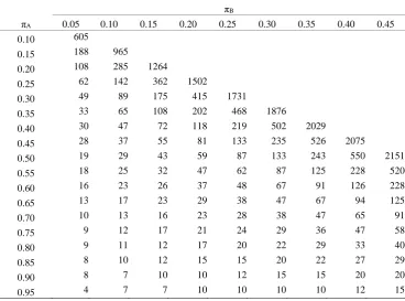
Table 7. Sample size estimates for one arm of a parallel group trial for various

expected outcome responses for a given treatment ( A) and comparator ( B) for a

one sided type I error rate of 2.5% and 90% power assuming Fisher’s exact test is the final analysis

B

A 0.05 0.10 0.15 0.20 0.25 0.30 0.35 0.40 0.45

0.10 605

0.15 188 965

0.20 108 285 1264

0.25 62 142 362 1502

0.30 49 89 175 415 1731

0.35 33 65 108 202 468 1876

0.40 30 47 72 118 219 502 2029

0.45 28 37 55 81 133 235 526 2075

0.50 19 29 43 59 87 133 243 550 2151

0.55 18 25 32 47 62 87 125 228 520

0.60 16 23 26 37 48 67 91 126 228

0.65 13 17 23 29 38 47 67 94 125

0.70 10 13 16 23 28 38 47 65 91

0.75 9 12 17 21 24 29 36 47 58

0.80 9 11 12 17 20 22 29 33 40

0.85 8 10 12 15 15 20 22 27 29

0.90 8 7 10 10 12 15 15 20 20

0.95 4 7 7 10 10 10 10 12 15

It is interesting to compare Table 6 with Table 7. The two tables are reasonably comparable and so if a Fisher’s exact test is to be considered for the final analysis it may be worth estimating the sample size using the more straightforward approach of the continuity corrected sample size calculation.

The programming for Table 7 is quite computer intensive. A quick estimate of the sample size for Fisher’s exact test can be obtained from a simple Normal approximation. If, in a study, we actually observed the predicted effect size, with the

required sample size at significance level and power 1- , then the observed test statistic is simply z1- +z1- For of 0.05 and of 0.10 the one sided P-value would

(26)

[image:26.595.90.464.135.404.2]

one sided P-value of 0.059% assuming Fisher’s exact test is the final analysis

B

A 0.05 0.10 0.15 0.20 0.25 0.30 0.35 0.40 0.45

0.10 615

0.15 204 977

0.20 113 298 1258

0.25 74 150 358 1514

0.30 55 92 179 429 1739

0.35 42 68 108 205 468 1896

0.40 37 49 74 124 227 507 2017

0.45 26 39 55 84 135 237 526 2095

0.50 23 31 45 59 87 137 243 545 2131

0.55 21 29 38 49 67 96 143 250 560

0.60 18 21 31 36 48 66 95 145 251

0.65 17 20 26 30 40 47 66 95 143

0.70 15 18 20 25 31 40 51 65 91

0.75 13 16 18 21 25 30 40 48 61

0.80 12 12 15 19 21 26 31 36 49

0.85 12 12 14 15 19 20 26 28 38

0.90 9 10 12 12 15 18 20 21 29

0.95 7 9 12 12 15 16 17 18 21

(27)

[image:27.595.90.500.513.721.2]

Figure 4. SAS code used to generate Table 8 for calculating sample sizes using only the P-value

data power;

do pa=0.10 to 0.95 by 0.05; do pb=0.05 to pa-0.45 by 0.05; flag=0;

p=round(10.5*(pa*(1-pa)+pb*(1-pb))/((pa-pb)*(pa-pb)))-1+3; do n=p to 10000 by 1 until (flag=10);

ka=round(pa*n); kb=round(pb*n); m=ka+kb;

prob=probhypr(2*n,m,n,kb); if prob lt 0.00059 then do; flag=flag+1;

end;

if prob ge 0.00059 and flag ge 1 then do; flag=0; end; end; n=n-flag+1; output; end;end;run;

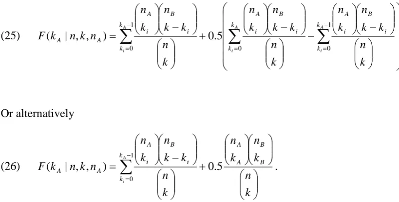
If we planned to use a mid-P P-value with Fisher’s Exact Test then Table 9 gives sample sizes for 90% power for a one tailed Type I error of 2.5%. This is calculated by amending equation (22) to become equation (25)

(25)                           −       −             −       +             −       =

∑

= − = − = A i A i A i k k k k i B i A i B i A k k i B i A A A k n k k n k n k n k k n k n k n k k n k n n k n k F 0 1 0 1 0 5 . 0 ) , , | ( Or alternatively

(26)

∑

− =                   +             −       = 1 0 . 5 . 0 ) , , | ( A i k k B B A A i B i A A A k n k n k n k n k k n k n n k n k F

(28)

[image:28.595.92.459.234.509.2]

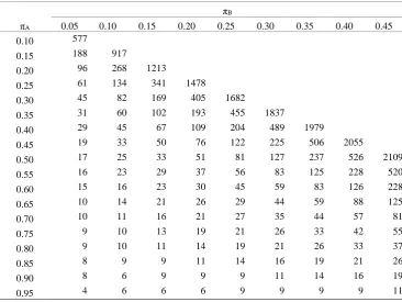
Comparing Table 9 to Table 7 we see there are bigger (in absolute terms) differences in the sample size estimates for the smallest effect sizes. The sample sizes estimated in Table 9 are closer to those of Table 5.

one sided type I error rate of 2.5% and 90% power assuming mid-P Fisher’s exact test is the final analysis

B

A 0.05 0.10 0.15 0.20 0.25 0.30 0.35 0.40 0.45

0.10 577

0.15 188 917

0.20 96 268 1213

0.25 61 134 341 1478

0.30 45 82 169 405 1682

0.35 31 60 102 193 455 1837

0.40 29 45 67 109 204 489 1979

0.45 19 33 50 76 122 225 506 2055

0.50 17 25 33 51 81 127 237 526 2109

0.55 16 23 29 37 56 83 125 228 520

0.60 15 16 23 30 45 59 83 126 228

0.65 10 14 21 26 29 44 59 88 125

0.70 10 11 16 21 27 35 44 57 81

0.75 9 10 13 19 21 26 33 42 55

0.80 9 10 11 14 19 21 26 33 37

0.85 8 9 9 11 14 16 19 21 26

0.90 8 6 9 9 9 11 14 16 19

0.95 4 6 6 6 9 9 9 9 11

We can repeat the quick method used in Table 8 for a mid-P value by replacing the line

prob=probhypr(2*n,m,n,kb);

with

prob=probhypr(2*n,m,n,kb-1)+0.5*(probhypr(2*n,m,n,kb)-probhypr(2*n,m,n,kb-1));

(29)

[image:29.595.95.461.132.404.2]

mid-P P-value 0.059% assuming Fisher’s exact test is the final analysis

B

A 0.05 0.10 0.15 0.20 0.25 0.30 0.35 0.40 0.45

0.10 580

0.15 186 916

0.20 99 265 1210

0.25 64 132 333 1462

0.30 45 81 160 391 1672

0.35 34 55 95 183 438 1840

0.40 27 41 64 107 202 475 1966

0.45 21 31 46 70 116 216 501 2050

0.50 17 24 34 50 76 123 225 517 2092

0.55 14 20 27 37 53 80 127 230 522

0.60 13 16 21 28 39 55 81 128 230

0.65 10 13 18 22 29 40 57 81 127

0.70 8 11 14 18 23 30 40 55 80

0.75 7 9 12 14 18 23 29 39 53

0.80 6 9 9 14 15 18 22 28 37

0.85 5 7 7 9 12 14 18 21 27

0.90 4 7 7 9 9 11 13 16 20

0.95 3 4 5 6 7 8 10 13 14

3.1.3. Worked Example 3 – Sample Size Calculation for a Parallel Group Superiority Trial with Binary Response

An investigator wishes to design a placebo controlled trial to investigate a new treatment for migraine. The absolute risk of migraine on placebo over the trial period is anticipated to be 50% and it would be clinically worthwhile using the drug if the risk was reduced on the new treatment to 40%. This is a treatment effect of an absolute risk reduction of 10%. The investigator wished to design the study to have 90% power and a two sided significance level of 5%.

The sample sizes using the different methods are given in Table 11.

(30)

gave a sample size of 542 patients per arm. A comparison of the results from nQuery with PASS and those in the paper are given in Table 11

In PASS to calculate the sample size you need to select “Proportions” and the “Two Groups: Independent” and finally “Inequality (Proportions)”. You can then drop down in the dialogue box “Test for” to calculate sample sizes for “Z-test unpooled” (equivalent to (18)); “Z-test pooled” (equivalent to (17)); “Z-test cc pooled” (equivalent to (17) and (21)) and “Fisher’s Exact Test”. For Fisher’s Exact Test though the calculation is only performed as default if the sample sizes in each arm are both less than 100. If this is not the case, then the continuity corrected calculations (equivalent to equations (18) and (21)) are undertaken. To change the default click on options and under “Exact Test Options” reset the “Maximum N1 or N2 for Exact Calculations”, for example to 10,000. For Fisher’s Exact test PASS gives a sample size of 533 patients per arm.

(31)

[image:31.595.92.498.201.587.2]

sample size of 533 before dropping below it again and re-crossing at 542 patients per arm.

Figure 5. Power for a given sample size for the case π_A=0.40 and π_B=0.50 for a Fishers Exact test for a one-sided Type I error rate of 2.5% from PASS.

(32)

[image:32.595.91.447.102.171.2]

Table 11. Comparison of results in paper with nQuery and PASS

Current Paper nQuery PASS

Normal Approximation from (18) 515 N/A 515

Normal Approximation from (17) 519 519 519

Continuity Correction from (17) and (21) 539 538 538

Fisher’s Exact Test 550 542 533

Fisher’s Exact Test Mid-P 526 N/A N/A

Our results are very slightly larger than those of nQuery for this worked example usingr Fisher’s Exact Test. For the continuity corrected sample size estimation PASS and nQuery give a sample size one less than the results in the paper. We suspect this may be due to the steps used for sample size calculation. For the Normal approximation using equation (18) both PASS and nQuery and this paper estimate the sample size to be 519 patients per arm. In actuality this was 518.04 rounded up to 519. If 519 is then used in (21) the sample size is estimated to be 539 patients. If 518.04 is used instead the sample size is 538 patients per arm.

3.1.4 Discussion of the Sample Size Calculations

There is a maxim that you should analyse your study as you have designed it. With sample size calculations it is the opposite way round – your design should reflect your planned analysis. Hence, if the plan is to undertake a chi-squared test for the primary analysis then a sample size calculation should reflect this. Thus, for both a single arm trial and a two arm trial depending on the assumptions for the analysis the planned statistical test should be considered [33,34]

We would recommend that the simple asymptotic approaches described here should be used for most sample size calculations. This does not preclude other approaches being used (including maybe simulations) to investigate the sensitivity of the initial calculations.

3.2. Non-Inferiority Trials

(33)

For certain trials therefore the objective is not to demonstrate that two treatments are different but rather to demonstrate that a given treatment is clinically not inferior compared to another. The null (H0) and alternative (H1) hypotheses for non-inferiority

trials may take the form:

H0: A given treatment is inferior with respect to the absolute risk of a response.

H1: A given treatment is non-inferior with respect to the absolute risk of a response.

A non-inferiority study is usually planned therefore to detect if the effect of the investigative treatment is not much worse than the control treatment defined by a non-inferiority margin, d. An assessment of non-non-inferiority of a new treatment is usually performed by comparing the lower tail of 95% confidence interval with the non-inferiority margin to rule out the non-inferiority of a new treatment. The threshold setting of d is not straightforward and is defined as the largest difference that is clinically acceptable such that a larger difference than this would matter in clinical practice [35]; a clinical judgement. This difference also cannot be “greater than the smallest effect size that the active (control) drug would be reliably expected to have compared with placebo in the setting of the planned trial” [36]; a statistical assessment. Often the margin is defined as some fraction of the active control effect (over placebo) to be retained and the control effect is estimated from historical trials as a statistical margin. Jones et al [31] recommend that the choice of limit be set at half the expected clinically meaningful difference between the active control and placebo as a clinical margin. For a binary outcome, the active control effect may be expressed as, the difference or difference in the logarithms in the event rates, or the difference in log-odds of the event of interest. Generally, the definition of an acceptable level of non-inferiority is made with reference to some retrospective superiority comparison to placebo [38-41]. In this context we layout the assumptions in a 2-arm non-inferiority trial and the issues with the non-inferiority margin [1,37-42]. There are regulatory guidelines on setting the non-inferiority margin [45,46].

Thus the two hypotheses become: H0: π_A −π_B ≤−d .

H1: π_A −π_B >−d.

In the context of non-inferiority trials –d is known as the non-inferiority limit. In order to conclude inferiority, we need to reject the null hypothesis. Thus, non-inferiority trials reduce to a simple one-sided hypothesis test. In practice, this is operationally the same as constructing a (1-2α)100% confidence interval and concluding non-inferiority provided that the lower end of this confidence interval is greater than –d.

(34)

1. The Assay sensitivity of the active control in both the placebo controlled trials and in the active controlled non-inferiority trial exists.

3. Bias is minimised through steps such as ensuring that the patient population and the primary efficacy endpoint are essentially the same for the placebo-controlled trial and the active-controlled trial.

2. Constancy assumption of the effect of the common comparator. For two trials in sequence, Trial 1 and Trial 2, the control effect of Treatment B vs. Placebo in Trial 1 is assumed to be the same as the control effect of Treatment B vs. ‘Placebo’ in Trial 2 In addition, to demonstrate that there is no clinically meaningful inferiority of the investigative treatment compared to the active control comparator, non-inferiority studies often entail an indirect cross-trial assessment. The indirect inference is that through comparing the investigative treatment to the control treatment, whether a new treatment preserves a fraction of the control effect or is superior to the ‘placebo’ not concurrently studied.

This is an issue, however, in that the estimate of effect over placebo in Trial 1 may possibly be overestimated for comparison in Trial 2 due to the placebo responses improving over time i.e. placebo ‘creep’. However the lack of constancy of control effect prescribed by the placebo ‘creep’ cannot be formally tested [38-44], although an educated assessment of constancy violation may help [49].

To ensure the choice of margin and hence to ensure the study is not biased, the following factors are critical in defining the non-inferiority margin:

i. How should the heterogeneity of the control effect and its variability across completed placebo-controlled trials, relative to Trial 1, be incorporated? ii. Should differential weight be given to the response from the most recent studies

and/or from the studies with smaller effects?

iii. What should be the preservation fraction be to account for the placebo ‘creep’?

From a public health perspective, when undertaking non-inferiority trials what we wish to do is to protect the efficacy that has been established with the standard therapy. This is as it is described for vaccination trials for example [50].

(35)

are used. For example consider Scenario 1 where two trials were conducted with the following regimens randomised.

Trial 1: Placebo and Treatment A, Trial 2: Placebo and Treatment B.

We could use the fact that both regimens have had a trial where they were compared to placebo to make comparisons between treatments A to B in the same patient population and the same primary efficacy endpoint studied.

Now consider Scenario 2 where Trial 1 and Trial 2 are conducted in sequence with the following set up.

Trial 1: Placebo and Treatment A, Trial 2: Treatment A and Treatment B,

Treatment A should have been shown to be effective in trial 1 (a placebo-controlled trial) in order to launch Trial 2 (an active-controlled trial). In some disease areas, when an approved agent becomes the standard of care it may no longer be ethical to conduct a placebo controlled trial. Thus, due to ethical constraints, Trial 2 cannot include a Placebo arm. In Scenario 2, comparison of A vs. B in Trial 2 is of primary interest, sometimes followed by the comparison of Treatment B vs. Placebo to indirectly infer efficacy of Treatment B through a cross-trial comparison.

In Scenario 2 a new treatment is compared to an established treatment with the objective of demonstrating that new treatment is non-inferior to this established treatment.

The methodologies for making indirect cross-trial comparisons are available, e.g., [38-51]. The validity of these methods relies on strong assumptions that often cannot be formally tested since treatments are not compared directly within the same trial [43-44].

3.2.1. Type I and setting the Non-inferiority Limit

3.2.1.1. Choice of Type I error

(36)

two sided 5% significance level, in practice for most trials what we have is a one sided investigation with a 2.5% level of significance. The reason for this is that we usually have an investigative therapy and a control therapy and it is only statistical superiority of the investigative therapy that is of interest.

Through the rest of the sections on equivalence and non-inferiority trials we will assume that α=0.025 and that 95% confidence intervals will be used in the final statistical analysis. This issue will be discussed again in the section on Bioequivalence.

3.3.1.2. Choice of Non-inferiority Limit

We have already discussed the setting of non-inferiority limits but general the following points should be considered:

1. You must be confident that the active control would have been different from the placebo had one been employed.

2. You should be able to determine that there is no clinically meaningful difference between the investigative treatment and the control treatment.

3. Through comparing the investigative treatment to the control treatment you should indirectly be able to determine that it is superior to placebo.

Steps 1 and 3 are important as there is a view that non-inferiority and equivalence (discussed later in the paper) trials reward "failed" studies i.e. if we conducted a poor trial where it would not have been possible to demonstrate the control treatment to be superior to placebo then a poor investigative therapy may be accepted by comparison to this control. However, Julious and Zariffa [54] point out that this may not be the case as poor studies are poor for most objectives as poor studies tend to have higher statistical variability and so are less likely therefore to show non-inferiority or equivalence.

We can therefore infer that the clinical difference used for the limits of equivalence and non-inferiority will be smaller than the difference used for placebo controlled superiority trials. There also is no generic definition for its setting – its definition will need to be defined on a study-by-study or indication-by-indication basis with consultation with the appropriate agencies and experts.

(37)

[image:37.595.94.429.103.174.2]

Table 12. Non-inferiority margins for different control response rates

Non-inferiority Margin

Response Rate FDA1 _CHMP2

≥90 -10% -10%

80-89% -15% -10%

70-79% -20% -10%

1_{Food and Drug Authority}2_{Committee for Health and Medicinal Products (formerly}

Committee for Pharmaceutical and Medicinal Products (CPMP))

Table 12 gives the non-inferiority margins for different response rates as recommended by FDA [55] and CHMP [56]. The FDA guidelines are redundant now but they do raise interesting points. What is evident from Table 12 is that whilst the CPMP recommend a flat equivalence margin, the FDA margins are a step function according to the anticipated control response rate.

3.2.2. Sample Size Calculation

The issue in calculating the sample size is that under both the null and alternative there is a non-zero difference between treatments. Generally, sample size formulas can be thought of as equation (27).

(27)

(

)

( )

( )2

2 1

1 Varianceunder Null Varianceunder theAlternative

d Z Z n B A A − − + = − − π π β α _.

Now (27) can be written

(28)

(

)

(

)

2

2 1 1 ) ( ) 1 ( ) 1 ( ) ~ 1 ( ~ ) ~ 1 ( ~ d Z Z n B A B B A A B B A A A − − − + − + − + − = − − π π π π π π π π π π _β α _,

where π~ and _A π~ are estimates of the responses on treatment under the null hypothesis _B used to estimate the variance under this hypothesis. For non-inferiority trials we have that π_A ≠π_B i.e. the two treatments do not have an equal response. As the estimates of

A

π and π_B effect the estimate of the variance the definition of the null hypothesis hence influences the variance under this hypothesis. There are a number of ways of considering this problem, three of which will now be discussed [3,57-60]. Julious and Owen [55] compared the different methods through simulation and within the parameters of the simulation recommended the simplest method for sample size estimation was to estimate the variance under the null hypothesis simply by replacing

A

[image:37.595.102.502.420.534.2]

(38)

(29) π_A(1−π_A)+π_B(1−π_B),

which is the same as the variance under the alternative.

For the special case of equal sized groups i.e.n_A =n_B , a direct estimate of the sample size can be obtained [57].

(30)

(

₍

)

(

₎

₂

)

2 1 1 ) ( ) 1 ( ) 1 ( d Z Z n B A B B A A

A ₋ ₋

+ − + − = − − π π π π π

π _β _α

.

where π_A is the assumed proportion of responses expected in subjects on treatment A andπ_B is the assumed proportion of responses in subjects on treatment B. Table 13 gives sample size estimates for 90% power and a type I error rate of 2.5%

As we discussed with superiority trials, equation (30) could be adapted to give the maximum sample size for the cases where π =0.5 (where π =(π_A +π_B)/2) [3]. Hence, a quick estimate of the sample size, for 90% power and two-sided significance level of 5%, can be obtained from the following result

(31)

(

)

2

) ( 25 . 5 d n B A A − − = π π .

While for 80% power and two-sided significance level of 5% the sample size can be estimate from

(32)

(

)

2

) ( 4 d n B A A − − = π π .

(39)

[image:39.595.96.529.118.462.2]

Table 13. Sample sizes for a non-inferiority study for 90% power and a type I error rate of 2.5%

A

B π

π −

A

π Limit -0.05 -0.04 -0.03 -0.02 -0.01 0 0.01 0.02 0.03 0.04 0.05

0.70 0.05 45845 11325 4993 2784 1766 1214 883 669 522 418

0.70 0.10 1839 1268 925 703 550 442 362 301 254 216 186

0.70 0.15 460 378 315 266 228 197 171 150 133 118 105

0.70 0.20 205 179 157 139 124 111 100 90 81 74 67

0.75 0.05 41537 10222 4491 2495 1577 1080 782 590 459 366

0.75 0.10 1671 1149 835 632 493 395 322 267 224 190 163

0.75 0.15 418 342 284 240 204 176 152 133 117 103 92

0.75 0.20 186 162 142 125 111 99 89 80 72 65 59

0.80 0.05 36178 8856 3872 2141 1345 917 660 495 382 303

0.80 0.10 1461 1000 723 545 423 337 273 225 188 158 135

0.80 0.15 366 298 246 207 175 150 129 112 98 86 76

0.80 0.20 163 141 123 108 95 85 75 67 60 54 49

0.85 0.05 29768 7227 3136 1720 1072 724 516 383 293 229

0.85 0.10 1209 822 590 441 340 268 216 176 145 121 102

0.85 0.15 303 245 201 167 141 120 102 88 76 66 58

0.85 0.20 135 116 101 88 77 67 60 53 47 42 37

0.90 0.05 22308 5336 2284 1234 757 502 351 255 190 145

0.90 0.10 915 615 436 322 244 190 150 120 97 79 65

0.90 0.15 229 183 149 122 101 85 71 60 51 43 37

0.90 0.20 102 87 74 64 55 48 41 36 31 27 24

Sample size estimates using equation (30) are given in Table 13 for the range 0.70

≤ A≤ 0.90 to illustrate the issues with non-inferiority sample size calculations. Note

that how for a trial being designed where the new treatment is thought to be a little better than control, i.e. π_B −π_A>0, the sample size is smaller than for π_B −π_A=0. The opposite is true for π_B −π_A<0.

Sample sizes are not given for anticipated responses greater than 0.90 as for high response rates the Normal approximation used in the sample size calculations may no longer hold. Our recommendation for sample sizes outside of this range would be to estimate the values using alternative methods such as simulation, which we describe below.

Tutorial in biostatistics: sample sizes for parallel group clinical trials with binary data

Tutorial in Biostatistics: Sample sizes for Parallel Group Clinical

Trials with Binary Data

Steven A. Julious and Michael J. Campbell

University of Sheffield

Contents

)

(

∑

∑

(

)

(

)

( )

( )

(

)

[

]

(

)

[

]

(

)

∑

∑

[

]

(

)

(

(

)

(

)

)

∑

(

)

(

)

(

)

[

]

(

)

(

)

(

)

(

)

∑

(

)

(

)

∑∑

∑

∑

∑

∑

(

)

(

)

(

)

(

(

)

(

)

)

(

)

(

₍

₎