A structural decomposition approach to
comparing MRIO databases
Anne Owen*1,Kjartan Steen-Olsen2, John Barrett1, Thomas Wiedmann3,4, Manfred Lenzen4
1 School of Earth and Environment, University of Leeds, Leeds, LS2 9JT, UK
2 Industrial Ecology Programme and Department of Energy and Process Engineering, Norwegian University of Science and Technology (NTNU), NO-7491 Trondheim, Norway
3School of Civil and Environmental Engineering, UNSW Australia, NSW 2052, Sydney, Australia 4Centre for Integrated Sustainability Analysis, School of Physics A28, The University of Sydney, NSW 2006, Australia
*Corresponding author: A. Owen, School of Earth and Environment, University of Leeds, Leeds, LS2 9JT, UK ([email protected])
Abstract
In the last five years there have been a number of global multi-regional input-output (MRIO) systems developed. The construction of MRIO tables involves the collection and manipulation of large datasets, and tables produced by different approaches may lead to different analytical outcomes. These differences can be described under three main areas: differences in the source data; differences in the choice of sector classification and/or regions; and methods employed to overcome missing information and to balance tables. In this paper we outline a decomposition methodology for investigating the variations that exist when using different MRIO systems to calculate the carbon dioxide (CO2) emissions induced by a region’s final demand. Structural decomposition analysis (SDA) attributes the change in emissions to a set of dependent determinants, such as technical coefficients, the Leontief inverse and final demands.
We apply our methodology to three prominent global MRIO databases – Eora, GTAP and WIOD – by aggregating them to a common classification system. Findings reveal that the variation between Eora and GTAP can be largely attributed to differences in the Leontief inverse and the emissions data, where-as the variation between Eora and WIOD is mainly due to differences in the final demand vector and the Leontief inverse matrix. For the majority of regions, GTAP and WIOD produce similar results and the variation can be attributed to the total output vector, the Leontief inverse matrix, the final demand vector and the composition of the final demand vector, respectively.
1. Introduction
The number of applications of multiregional input-output (MRIO) databases to policy analysis and appraisal has steadily increased (Galli et al., 2012; Wiedmann and Barrett, 2013; Springmann 2014). At the same time a number of global MRIO databases have been developed. One of the key applications of these databases is to provide consumption-based emissions accounts for various regions and countries from the global perspective (Hertwich and Peters, 2009; Wiedmann, 2009; Wiedmann et al., 2011; Tukker and Dietzenbacher, 2013) but there is obvious variation in the analytical results (Barrett et al., 2013; Peters et al., 2012; Sato, 2012). From the perspective of policy application this variation could raise concerns and imply a need for caution when interpreting the results (CCC, 2013).
With each MRIO database being the culmination of different sets of source data, structures and modelling methodologies; it is not surprising that different analytical outcomes are observed. The challenge for researchers in the field of MRIO analysis is to explain and understand the variation in results. Developing a methodology for measuring and understanding the variation is paramount. In this paper we apply structural decomposition analysis (SDA) methods to explore variation and propose a transparent approach to explaining these differences.
1 denotes matrix diagonalisation
2. Methods and Data
2.1. Multiregional input-output databases
Input-output (IO) methods have been used to link environmental impacts associated with production to the consumption of final products. The Leontief IO model is constructed from IO tables and shows the interrelationships between industries and products (Miller & Blair, 2009). The Leontief equation,
𝐱 = (𝐈 − 𝐀)−𝟏𝐲 (1)
describes output (𝐱) as a function of final demand (𝐲).𝐈 is the identity matrix, and𝐀is the technical coefficient matrix, which shows the direct inter-industry requirements. (𝐈 − 𝐀)−𝟏 is known as the Leontief inverse (denoted hereafter as 𝐋). 𝐋 is sometimes referred to as the total requirements matrix, as each element in its column gives the total inputs required for producing one unit of output of the sector associated with that column. Since the 1960s, the IO framework has been extended to account for increases in the pollution associated with industrial production due to a change in final demand (Bjerkholt and Kurx, 2006; Miller & Blair, 2009).
Consider, a row vector𝐟of annual CO2emissions generated by each industrial sector
𝐞𝐜= 𝐟𝐱−𝟏 (2)
is the coefficient vector representing emissions per unit of output1. Multiplying both sides of (1) by 𝐞𝐜gives
𝐞𝐜𝐱 = 𝐞𝐜𝐋𝐲 (3)
and simplifies to
𝑞 = 𝐞𝐜𝐋𝐲 (4)
Total emissions 𝑞 are calculated by pre-multiplying 𝐋 by emissions per unit of output and post-multiplying by final demand. Equation (4) can be used to analyse how a change in the final demand of goods and services would change the economy-wide CO2emissions,ceteris paribus. Emissions are reallocated from production sectors to the final consumption activities. The emissions of each sector required in the production of a particular product are reallocated to the demand of this product, rather than the supply. In other words, we can show the emissions associated with final consumption.
countries/regions, that there is a degree of harmonisation in sectors described and that data on the imports to intermediate demand can be either found or calculated (Tukker et al., 2009). In the last five years, several global MRIO databases capable of tracking flows of goods and services between regions have been developed (Hertwich and Peters, 2009; Minx et al., 2009; Wiedmann, 2009; Peters and Solli, 2010; Wiedmann et al., 2011; Lenzen et al., 2012a; Andrew and Peters, 2013; Dietzenbacher et al., 2013; Lenzen et al. 2013; Meng et al., 2013; Tukker et al., 2013; Tukker and Dietzenbacher, 2013;).
Environmentally extended MRIO (EE-MRIO) techniques have numerous policy applications; the calculation and reporting of consumption-based emissions accounts being one (Minx et al., 2009; Barrett et al., 2013; Wiedmann and Barrett, 2013). National greenhouse gas (GHG) emissions reports usually account for the carbon emissions from production activities within the country’s territory (United Nations, 1992, Article 12, p.15). Results from MRIO databases allow for a contrasting perspective; a consumption-based account can quantify those emissions occurring in foreign regions to satisfy domestic final consumption and similarly quantify the proportion of domestic emissions embodied in products for export (Peters, 2008; Peters and Hertwich, 2008a; Hertwich and Peters, 2009; Wiedmann, 2009; Davis and Caldeira, 2010; Davis et al., 2011; Wiedmann et al., 2011; Jakob and Marschinski, 2013).
2.2. MRIO databases currently available
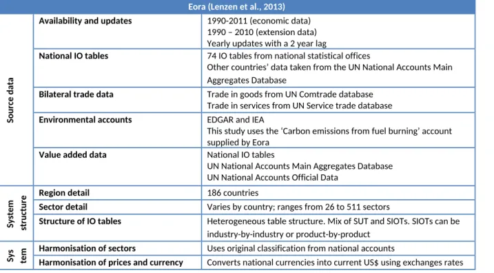
The latest reviews of the main global MRIO initiatives (Peters et al., 2011; Wiedmann et al., 2011; Andrew and Peters, 2013; Dietzenbacher et al., 2013; Lenzen et al., 2013; Meng et al., 2013; Tukker et al., 2013; Tukker and Dietzenbacher, 2013), describe five MRIO databases: EXIOPOL, GTAP, Eora, AIIOT and WIOD. The year 2007 has been chosen for this study because it is the latest year where there are at least three MRIO databases to compare. Table 1 (adapted from Steen-Olsen et al., 2014b) provides summary information about the source data and construction techniques used in building the databases
Table 1 Global MRIO databases used for comparisons in this study and their features
Eora (Lenzen et al., 2013)
Source
data
Availability and updates 1990-2011 (economic data) 1990 – 2010 (extension data) Yearly updates with a 2 year lag
National IO tables 74 IO tables from national statistical offices
Other countries’ data taken from the UN National Accounts Main Aggregates Database
Bilateral trade data Trade in goods from UN Comtrade database Trade in services from UN Service trade database Environmental accounts EDGAR and IEA
This study uses the ‘Carbon emissions from fuel burning’ account supplied by Eora
Value added data National IO tables
UN National Accounts Main Aggregates Database UN National Accounts Official Data
System structure
Region detail 186 countries
Sector detail Varies by country; ranges from 26 to 511 sectors
Structure of IO tables Heterogeneous table structure. Mix of SUT and SIOTs. SIOTs can be industry-by-industry or product-by-product
from IMF Off-diagonal trade data calculations,
balancing and constraints Large-scale KRAS optimisation of an initial MRIO estimate withvarious constraints
GTAP (Andrew and Peters, 2013)
Source data
Availability and updates 2001, 2004, 2007
Updated on a 3 year interval with a 4 year lag National IO tables Tables submitted by GTAP consortium members Bilateral trade data Trade in goods from UN Comtrade database.
Trade in services from UN Service trade database Environmental accounts CO2derived from IEA energy data.
This study uses the data supplied by GTAP v7.1 which includes CO2 from fossil fuel burning only (Lee, 2008)
Value added data Tables submitted by GTAP consortium members
System structure
Region detail 129 regions (81 for 2001)
Sector detail 57 homogeneous product-by-product sector tables
Structure of IO tables Homogenous SIOT table structure
System
construction
Harmonisation of sectors To disaggregate a country’s non-agricultural sectors, the structure from other IO tables within regional groupings is used. For agricultural sectors data from the FAO is employed
Harmonisation of prices and currency IO tables scaled to US$ using GDP data from the World Bank Off-diagonal trade data calculations,
balancing and constraints Uses ‘entropy-theoretic methods’ to harmonise dataset. Constraintsinclude consumption data from the World Bank, energy data from IEA, bilateral trade data from UN’s COMTRADE database.
WIOD (Dietzenbacher et al., 2013)
Source
data
Availability and updates 1995 – 2011 (economic) 1995-2009 Environmental Funding dependent
National IO tables SUTs from National Accounts.
Bilateral trade data Trade in goods from UN Comtrade database. Trade in services from UN, Eurostat and OECD Environmental accounts Emissions from NAMEA
Value added data SUTs from National Accounts.
System structur e
Region detail 40 countries and a rest of the world region Sector detail 35 homogeneous industry-by-industry sector tables Structure of IO tables Homogenous SIOT table structure
System
construction
Harmonisation of sectors Developed concordance tables between national classifications and the 35 sectors used in WIOD.
Harmonisation of prices and currency Supply table (from SUT) in basic prices. Use table in purchases prices. Transform the Use table to basic prices.
Convert all data to current US$ using exchange rate from IMF Off diagonal trade data calculations,
balancing and constraints International SUTs merged to a ‘World SUT’ then transformed to aWIOT using the fixed product sales structure assumption.
2.3. Emissions data
2Version 199.74
investigation of the effect on consumption-based accounts when different emissions data is included.
In the present study we decided to use CO2emissions from fossil fuel burning only. This is not because we believe this to be the most appropriate measure for calculating consumption-based emissions account. Rather, fossil-fuel combustion data are found consistently in the extension datasets provided with MRIO databases, keeping variation to a minimum. Eora has over 40 extension datasets of which CO2from fuel burning is one. The CO2emissions data provided with GTAP v7.1 is emissions from fuel burning only (Lee, 2008). WIOD however, uses NAMEA data for its CO2 extension dataset. This includes cement production but no other process emissions (Genty et al., 2012; Peters el al., 2012).
Despite our efforts to ensure that the emissions data is consistent across the datasets, Table 2 shows that the total CO2differs substantially between them. Therefore, in what follows, total emissions will be treated as one of the independent variables in determining the variation in consumption-based emissions.
This study aims to discover how much of the outcome variation is due to a difference in the total emissions used in the databases and how much is due to the distribution of emissions.
Table 2: Comparison of total CO2emissions in Eora, GTAP and WIOD 2007
Eora GTAP WIOD
Total Global emissions
2007 (ktCO2) 28,237,228 22,800,300 25,261,657
2.4. The aggregated MRIO databases used in this study
For this study, we compare CO2emissions associated with final consumption calculated for the year 2007 using the Eora2, GTAP and WIOD MRIO databases. The SDA techniques described in section 2.5 require the multiplication of matrices which share a common structure. This means that the number of regions and sectors must be the same and presented in the same order. To construct an equation that takes elements from one MRIO database and elements from a second requires either a complex system of concordance matrices or some pre-calculation reclassification and aggregation to ensure that the matrices involved are the same size and structure.
For a more detailed discussion on the methods employed to construct the aggregated systems see Steen-Olsen et al (2014a).
2.5. Uncertainty analysis in input-output analysis
This study aims to explore the variation in consumption-based emissions calculated by different MRIO databases and sits within the field of model uncertainty assessments. Uncertainty assessments of the outcomes of models to predict future global emissions exist and the recently published contribution of Working Group I to the Fifth Assessment Report of the Intergovernmental Panel on Climate Change (Stocker et al., 2013) gives a clear explanation on how model results can be quantified in terms of their uncertainty. However, as Lenzen et al. (2010) and Wiedmann (2009) note, there are few examples of environmental MRIO studies where uncertainty analyses have been undertaken. Lenzen et al. (2010) collect standard deviations associated with the underlying source data that is used to make the UK IO accounts and then regress the standard deviations across the values in the supply and use tables, eventually calculating a total relative standard error of the MRIO table (Lenzen, 2000). However, the standard errors of the Leontief Inverse 𝐋 cannot be calculated analytically (Lenzen, 2000) and Monte-Carlo techniques must be used.
Monte-Carlo methods involve propagating repeated random input variables through a calculation and observing the effect on the output (Peters, 2007). Monte Carlo techniques have been used to estimate an 89% probability that the UK’s carbon footprint increased between 1994 and 2004 (Lenzen et al., 2010) and to show that while uncertainties around the total Dutch carbon footprint were low, lower tiered impacts attributed at the regional and sector level contained higher uncertainty (Wilting 2012). One drawback of using this method to understanding uncertainty in MRIO analysis is the assumption that errors in the table are normally distributed and independent of each other (Lenzen 2000). The nature and construction constraints of an MRIO table mean that this is not the case. Monte-Carlo analysis may not deal with systematic errors associated with the build assumptions made by model developers, such as currency conversion factors, imports structures and balancing approaches (Lenzen et al., 2010).
One method for understanding the effect of build assumptions is to construct several versions of the MRIO table, each with different build techniques, and observe the effect on output. For example, Peters and Solli (2010) investigate aggregation effects by quantifying the difference in Nordic countries footprints using the GTAP data with eight aggregated sectors and then the full 57 sectors. Weber and Matthews (2007) show that the choice of currency conversion method used for certain developing countries greatly affects the size of emissions embedded in imports to the US. In addition, Peters et al (2012) investigate how model outcomes change when different CO2emissions data are used with the GTAP MRIO table, concluding that much of the variation in outcome may be due to differences in extension data.
It is important to understand the effect of uncertainty in source data and the effect different build assumptions have on a system’s output. However, the assessments described above do not consider the variations between the MRIO databases themselves, which is an important factor. This study employs SDA techniques to address this.
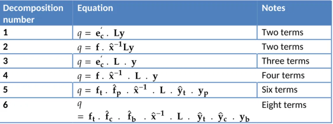
2.6. Structural Decomposition Analysis
3 Dietzenbacher and Los (2000) warn that analyses that decompose total value added need to be treated with care due to the dependency problem. The equation used is similar to (4) with𝑞 replaced by total value added 𝐯, and 𝐞`𝐜 representing sectoral value added per unit of output. A
decomposition equation containing three terms, 𝐞`𝐜, 𝐋 and 𝐲 assumes that ∆𝐞`𝐜, and ∆𝐋 are independent. The authors point out that “changes in intermediate input coefficient and in value added coefficient affect each other” (Dietzenbacher and Los, 2000 p4). SDA applied to measures of consumption-based emissions require the calculation of the emissions per unit of output and this dependency issue will need to be considered. It is not appropriate to assume that a change in emissions efficiency can occur independently of the technology matrix used to calculate𝐋.
SDA takes the component parts of the fundamental Leontief equation (1) and calculates the effect each term has on an economic change. If the Leontief equation is the product of three terms there are a total of six, (3! = 6), decomposition equations that can be formulated to describe the change in output (see SI for further details). This means that there is no unique solution and each of the decomposition forms is equally valid (Dietzenbacher and Los, 1998). This is known as the non-uniqueness issue. The mean of each of the decomposition solutions is often taken as an indication of the influence of each term but Dietzenbacher and Los, (1998) note that the maximum, minimum and standard deviation of each term should also be reported.
Rather than calculating the drivers of a change in economic output, we use the environmentally extended Leontief equation (4) and consider change in emissions (∆𝐟)3. The use of SDA to understand the drivers of emissions change over time is well documented. Studies investigating the causes of a nation's increase in carbon footprint include Guan et al. (2009), Baiocchi and Minx (2010), Minx et al. (2011) and Tian et al., (2014). Both Baiocchi et al. (2010) and Minx et al. (2011) report the calculated ranges for each term and Minx et al. (2011) find the influence of the change in the𝐋term to be particularly large. Other SDA studies include investigation into energy use change (Rose and Chen, 1991; Wachsmann et al, 2009; Weber, 2009; Zhang and Lahr, 2014) and GHG emissions change (Wood, 2009; Brizga et al., 2014). Instead of using SDA to understand the drivers of change overtime, this analysis considers the drivers of the variation in emissions calculated by a pair of different MRIO databases for the same year. Thus, rather than ∆𝑞 representing a change in emissions between time𝑡1and𝑡2,∆𝑞is now the difference in emissions calculated between MRIO 1 and MRIO 2. There is a precedent for using decomposition techniques to assess uncertainties in climate model projections. Déqué et al. (2007) consider the uncertainty in climate response predictions and decompose uncertainty into four factors: sampling uncertainty; model uncertainty; radiative uncertainty; and boundary uncertainty. Our study does not attempt to quantify uncertainty around MRIO databases; rather it aims to decompose model outcome variation into contributions from the emissions source data and contributions from the economic trade table.
2.7. Difference equations
(𝐱−𝟏). The reason for this is twofold. Firstly, the emissions vector and total output are often taken from two different data sources and their separate contribution to total database variation should be investigated. Secondly, this removes the efficiency vector from the equation which would be dependent on the technology matrix (Dietzenbacher and Los, 2000). This amendment does not follow the proposed form suggested by Dietzenbacher and Los (2000) for cases with dependent determinants. There is no simple way of amending the terms to create independency and we highlight that the dependency issue is problematic for all SDA that assess changes in emissions and energy (Minx et al., 2011). The approach outlined in this study is, however, applied consistently across the pairings investigated and allows for comparisons to be made. The equations calculated and terms used are summarised in Table 3.
Table 3 SDA equations used in this study
Decomposition
number Equation Notes
1 𝑞 = 𝐞`𝐜 . 𝐋𝐲 Two terms
2 𝑞 = 𝐟 . 𝐱−𝟏𝐋𝐲 Two terms
3 𝑞 = 𝐞`𝐜 . 𝐋 . 𝐲 Three terms
4 𝑞 = 𝐟 . 𝐱−𝟏 . 𝐋 . 𝐲 Four terms
5 𝑞 = 𝐟𝐭 . 𝐟𝐩 . 𝐱−𝟏 . 𝐋 . 𝐲𝐭 . 𝐲𝐩 Six terms
6 𝑞
= 𝐟𝐭 . 𝐟𝐜 . 𝐟𝐛 . 𝐱−𝟏 . 𝐋 . 𝐲𝐭 . 𝐲𝐜 . 𝐲𝐛
Eight terms
𝐟𝐭 Row vector where each element is equal to the total global CO2emissions. Dimensions [1 ×
mn]
𝐟𝐜 Diagonalised vector of the proportion of total global CO2 emissions that each country’s
production emissions represents. The first mvalues each show the repeated proportion of total emissions attributed to region 1, the nextm, region 2 etc. Dimensions [mn × mn]
𝐟𝐛 Diagonalised vector of the proportion of each country’s total production emissions each domestic industrial sector represents (basket of production emissions). The first mvalues are the proportions for region 1, the nextm, region 2 etc. Dimensions [mn × mn]
𝐟𝐩 Diagonalised vector of the proportion of global CO2 emissions that each global production
sector represents. Dimensions [mn × mn]
𝐟 Row vector of production emissions by region and sector. Dimensions [1 × mn]
𝐞`𝐜 Row vector of production emissions per unit of output by region and sector. Dimensions [1 × mn]
𝐲 Column vector of final demand of the region being calculated; by region and sector. Dimensions [mn × 1]
𝐲𝐭 Diagonalised vector where each element is equal to the total final demand of the region
being calculated. Dimensions [mn × mn]
𝐲𝐩 Column vector of the proportion of the total region’s final demand that each global product
represents. Dimensions [mn × 1]
𝐲𝐜 Diagonalised vector of the proportion of the region’s total final demand that is supplied by
each import country. The first m values each show the repeated proportion of total final demand supplied by region 1, the nextm, region 2 etc. Dimensions [mn × mn]
𝐲𝐛 Column vector of the proportion of each product that makes up a single import regions
supply to final demand (basket of products). The first m values are the proportions for region 1, the nextm, region 2 etc. Dimensions [mn × 1]
3. Results
We first investigate the effect of the aggregation classification systems on the CO2 emissions assigned to the final demand of the 40 countries in the CC for the year 2007, and then investigate the results from the SDA.
3.1. Effect of aggregation
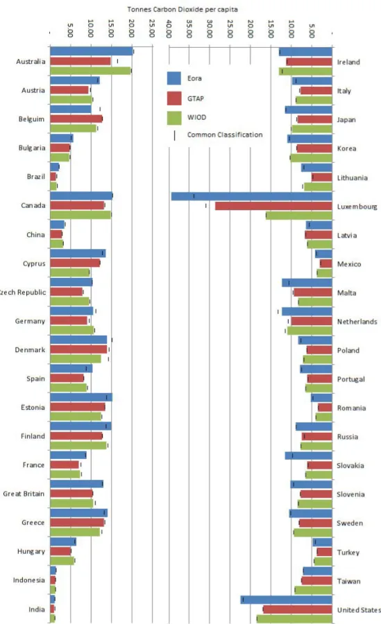
Figure 1 shows the per-capita consumption-based CO2 emissions of each of the 40 countries in the CC as reported by Eora, GTAP and WIOD. Black bars show the calculated emissions using the CC. The chart has a per-capita scale to allow data from small countries to be seen alongside larger ones. The per country consumption-based emissions reported by the CC is on average 6% different to the original Eora, 3% different to the original GTAP and 2% different to the original WIOD, reflecting the fact that the CC is most similar to the WIOD database. The country with the greatest variation to the original is Belgium’s Eora CC at 19%. Table S9 in the SI gives further information for all regions and all aggregations. As expected the PC systems produce results closer to their originals with the WIOD PC being 0.7% different on average. The effect of the aggregation is similar to results presented by Peters and Solli (2010) who find that compared to the full GTAP MRIO, an aggregated version with 8 sectors gives variations of up to 19% for Cambodia but just 1 to 3% for the Nordic countries. The authors conclude that if the primary interest is footprint totals “only a modest level of sector detail is necessary” (Peters and Solli, 2010 p50). Similarly, Peters and Solli (2010) show that MRIO databases can give reasonable results when aggregated to just the five to ten most important trading regions. Figure 1 also shows the difference between the emissions reported by the three databases. Luxembourg, in particular, displays very different per-capita emissions from a consumption-based perspective; results from this study may help explain why.
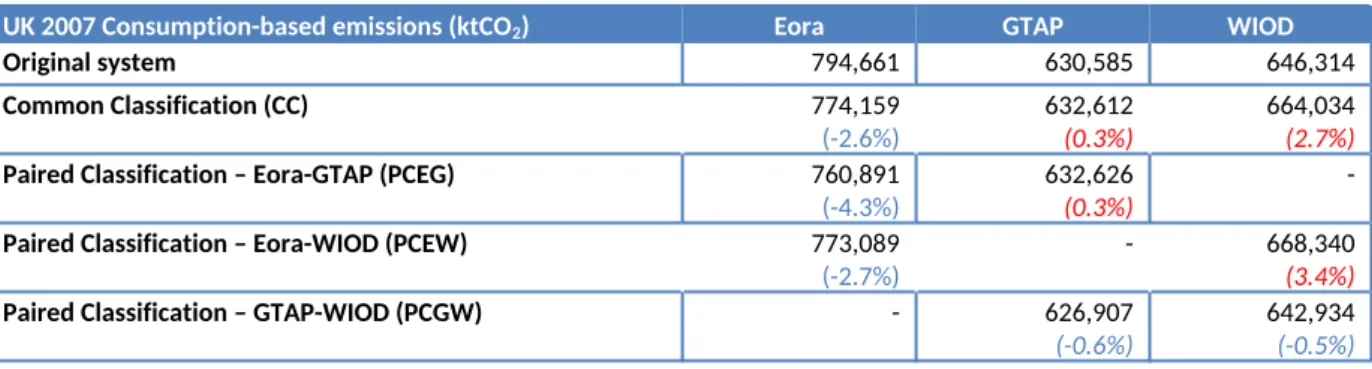
Since it is beyond the scope of a journal paper to interpret results from every country in the CC, we use the UK as a case study when interpreting the SDA results. The UK has a history of consumption-based accounting (Wiedmann et al., 2008; Minx et al., 2009; Lenzen et al., 2010; Wiedmann et al., 2010; Wiedmann et al., 2013; Barrett et al., 2013) and the results calculated for the UK using the aggregated databases are close to the original values (Table 4). All variations are within or below the reported standard deviation of the UK-MRIO database reported by Lenzen et al (2010). We therefore establish that the aggregated systems used in the present study are a reasonable representation of the original MRIO databases for the UK. For a more detailed discussion on the effects of these aggregation systems see Steen-Olsen et al. (2014a).
Table 4 Effects of aggregation on calculation results for the UK 2007 carbon footprint (values in brackets show relative increase or decrease in results compared to the un-aggregated database)
UK 2007 Consumption-based emissions (ktCO2) Eora GTAP WIOD
Original system 794,661 630,585 646,314
Common Classification (CC) 774,159
(-2.6%) 632,612(0.3%) 664,034(2.7%)
Paired Classification – Eora-GTAP (PCEG) 760,891
(-4.3%) 632,626(0.3%)
-Paired Classification – Eora-WIOD (PCEW) 773,089
(-2.7%) - 668,340(3.4%)
Paired Classification – GTAP-WIOD (PCGW) - 626,907
3.2. Consumption-based emissions variation
The SDA equation will attribute the emissions variation to a set of determinants. Table 5 shows the variation for the UK for each pair of MRIO systems. For the UK, pairs involving Eora reveal highest variation and the PC has the effect of reducing variation size. The variation for each of the 40 countries is shown in Table S10 in the SI.
Table 5 Variation in calculated consumption-based CO2emissions for the UK
KtCO2 Eora - GTAP Eora - WIOD GTAP - WIOD
Common Classification (CC) 141,548 110,125 -31,423
Paired Classification (PC) 128,265 104,749 -16,026
This variation is thenetdifference between the databases and may actually be the composite of a series of contributing differences both positive and negative. Using full SDA techniques we attempt to calculate the gross difference between the two MRIO databases in question and break this difference down to the sum of individual element-wise contributions. We appreciate that there is no unique solution to the gross difference (Dietzenbacher and Los, 1998) and our decision to use the mean solution is just one of many possible outcomes. However, using the mean is a common compromise (Baiocchi et al., 2010; Minx et al., 2011) and we use this consistently throughout the study.
3.3. SDA results
This section summarises our findings by means of a series of questions. Detailed results from a large number of permutations (three databases, two classification systems and six SDA equations) can be found in the SI.
3.3.1.How can the findings be interpreted?
We use the Eora-WIOD UK comparison with the common classification as an example of how to interpret results. The SDA calculates the mean, maximum and minimum contribution that each term makes towards the emissions variation. If a term has a positive contribution it can be interpreted that switching that variable from the WIOD term to the Eora term increases the footprint on average by that amount. If the term has a negative contribution, a switch from WIOD to Eora contributes to lowering the footprint.
Figure 2 shows results of the SDA for the Eora-WIOD pairing under the CC as a stacked bar chart where the bars show the mean contributions of each of the terms and the error bars indicate the maximum and minimum contribution each term makes towards the emissions variation (see also Table S13 in the SI). The net difference, of 110,125 kt CO2is the sum of each column. For the first decomposition, the CO2per unit output (𝐞`𝐜) contributes a mean of 95% of the net difference and the product of the Leontief matrix and the UK’s final demand vector (𝐋𝐲) makes up the remaining 5%. For this decomposition 𝐞`𝐜 is the driving factor of Eora’s larger emissions estimate. As the Leontief
consumption-based account for the UK. The total UK final demand reported in WIOD has the effect of producing a larger UK impact than the Eora UK final demand but this positive driver is cancelled by emissions and economic structure.
Figure 2: SDA decompositions of variation in UK consumption-based CO2emissions between Eora and WIOD in CC The mean effect of each term is just one solution to the SDA breakdown. Results must also be interpreted alongside the minimum, maximum and standard deviation calculated for each term. Consideration of this additional information allows comment on the reliability of findings.
3.3.2.How much variability surrounds difference calculation?
We take the sixth and most detailed decomposition from Figure 2, and focus on the contribution from each of the terms. Table 6 shows that𝐋, 𝐟𝐭 ,𝐱−𝟏and 𝐲𝐭 have the largest mean contributions.
However the size of the effect of, 𝐱−𝟏 can range from -10,611 to -139,319 and the 40,320 (8!) combinations used to calculate the effect of this term have a standard deviation of 44,464. The standard deviation of𝐋is equally as large but𝐲𝐭 exhibits a smaller range of possible outcomes and a
lower standard deviation.
Table 6: Full SDA results for the Eora-WIOD comparison of UK consumption-based emissions (kt CO2)
𝐟𝐭 𝐟
𝒄 𝐟𝒃 𝐱−𝟏 𝐋 𝐲𝐭 𝐲𝐜 𝐲𝐛
𝐟 80,703 6,971 -18,009 -65,267 177,519 -30,656 249 -41,385 𝐟𝐦𝐚𝐱 103,909 13,669 -1,898 -10,611 268,394 -23,697 4,389 -6,862 𝐟𝐦𝐢𝐧 64,730 2,486 -58,825 -139,319 102,435 -40,763 -3,657 -75,352 𝛔𝐟 9,290 2,292 14,732 44,464 42,856 4,096 1,924 19,383
𝐲𝐛
𝐲𝐜
𝐲𝐩
𝐲𝐭
𝐟𝐩
𝐟𝐛
𝐟𝐜
𝐟𝐭
𝐲
𝐋𝐲 𝐋
𝐱−𝟏𝐋𝐲
𝐞𝐜
A students’ t-test on the means of each of the terms in the sixth decomposition equation for each of the six pairings, finds that they are significant at the .01 level. This is to be expected with such a large sample used to calculate the mean and we can be confident that there is little uncertainty associated with our calculation of the mean values. This finding reinforces the strength of the SDA methods described by Dietzenbacher and Los (1998) and used in our study. Considering every possible combination of decomposition equations ensures that a mean is calculated with greater certainty than taking the polar decompositions or some other selection of equations.
The range of possible outcomes for the effect of each term is larger for some terms than others and we suggest that any interpretation of SDA results requires consideration of the full range of outcomes rather than a simple reporting of the mean. Figure 3 suggests an example as to how these SD results could be presented. The chart shows the term-wise breakdown of the sixth SDA equation of the variation in UK consumption-based emissions between Eora and WIOD under the CC. The columns represent the mean contribution from each term and the net difference is the sum of all the columns. Clearly, some terms contribute positively to the variation and some negatively. The solid black lines represent the maximum and minimum contribution to the variation from each term in the decomposition equation. We present a single mean solution to the contribution each term makes, but the solution may deviate between the maximum and minimum points. Due the fact that each SDA difference equation has the same net total, if one solution contains the maximum of one of the terms, the remainder of the terms need to be low in comparison. This means that solutions will never lie along the path of the maximums but somewhere in between.
𝐟𝐭and𝐲𝐭draw from narrow ranges of possible outcomes across all pairings whereas𝐱−𝟏,𝐟𝐛,𝐋and
𝐲𝐛have the widest. The 𝐟𝐭 term has a large effect on database variation but draws low range of
Figure 3: Breakdown of the variation between Eora and WIOD CC UK including maximum and minimum values
The tables for the other five pairings can be interpreted similarly and this type of analysis can be performed for all other countries in the CC (see SI).
3.3.3.Can findings be linked to source data and construction methods?
To fully understand which components are the causes of variation in consumption-based emissions results, the SDA findings need to be viewed alongside the MRIO metadata shown in Table 1. For example, Eora-WIOD variations for the UK seem to be due to a difference in total emissions but not by emissions distribution by region or industrial sector. Table 1 confirms that Eora and WIOD use emissions data from different sources and Table 2 highlights the difference in total emissions. Variation from 𝐱−𝟏, 𝐋and 𝐲terms will be a combination of differing source data and construction methods used to make the MRIO table. Table 1 shows that although Eora and WIOD source the
𝐟′
𝐭𝐟
𝐜𝐟
𝐛𝐱
−𝟏𝐋
𝐲
𝐛𝐲
𝐜𝐲
𝐭 Total netdifference Net
variation 𝐲𝐛
𝐲𝐜
𝐲𝐭
𝐟𝐭
𝐟𝐜
𝐟𝐛 𝐋
domestic tables from national accounts and the trade data from UN Comtrade, Eora keeps the data in its original format whereas WIOD uses concordance matrices to transform the data to a common sector classification. This will be one of the reasons for the variation. In addition most elements in an MRIO table represent interregional transactions (off-diagonal blocks) and the method used to populate these table elements will have a large effect on𝐋. Clearly SDA can have a role in indicating which elements of the Leontief equation contribute most to model difference. However, further investigation is needed to quantify the relative contribution by source data and construction techniques to outcome difference.
3.3.4.Which MRIO pairings are most and least similar?
In Figure 2, the gross difference is the length of the entire stacked column. The gross difference is not the same value for each of the decompositions. However since the mean is drawn from a sample of over 40,000 results and we apply the same difference equations to all pairings, we argue that this consistent approach allows comment on the findings from calculating the gross difference.
Using the estimated gross differences using the mean of the terms from the sixth decomposition, we can predict which of the MRIO pairings has the highest variation. This pairing can be described as the least similar. Table 7 shows, 17 out of 40 countries show the Eora-GTAP PC pairing to be the least similar and for 16 out of 40 countries, the GTAP-WIOD PC pairing is the most similar. Table S17 in the SI shows which pairing is most similar for each country.
Table 7: Number of countries where each of the MRIO database pairings is most and least similar
Eora-GTAP CC Eora-GTAP PC Eora-WIOD CC Eora-WIOD PC GTAP-WIOD CC GTAP-WIOD PC Number of countries where
pairing is least similar (20%)8 (43%)17 (15%)6 (15%)6 (0%)0 (8%)3
Number of countries where
pairing is most similar (0%)0 (0%)0 (15%)6 (15%)6 (30%)12 (40%)16
3.3.5.Which factor contributes most to the variation in footprint results?
Figure 4 shows the mean contribution by each term to the gross emissions variation for each country for the three database pairings in the CC (using the sixth decomposition). For example, the variation in the emissions calculated for France between Eora and GTAP seem to be mainly due to differences in the total emissions vector. For Luxembourg, where the consumption-based emissions are very different (Figure 1), total final demand appears to be an important contributor towards the variation between all MRIO pairings. When selecting a database to provide information about Luxembourg’s consumption-based emissions, policy makers might want to consider which database contains final demand data for Luxembourg that is closest to the nation’s national accounts.
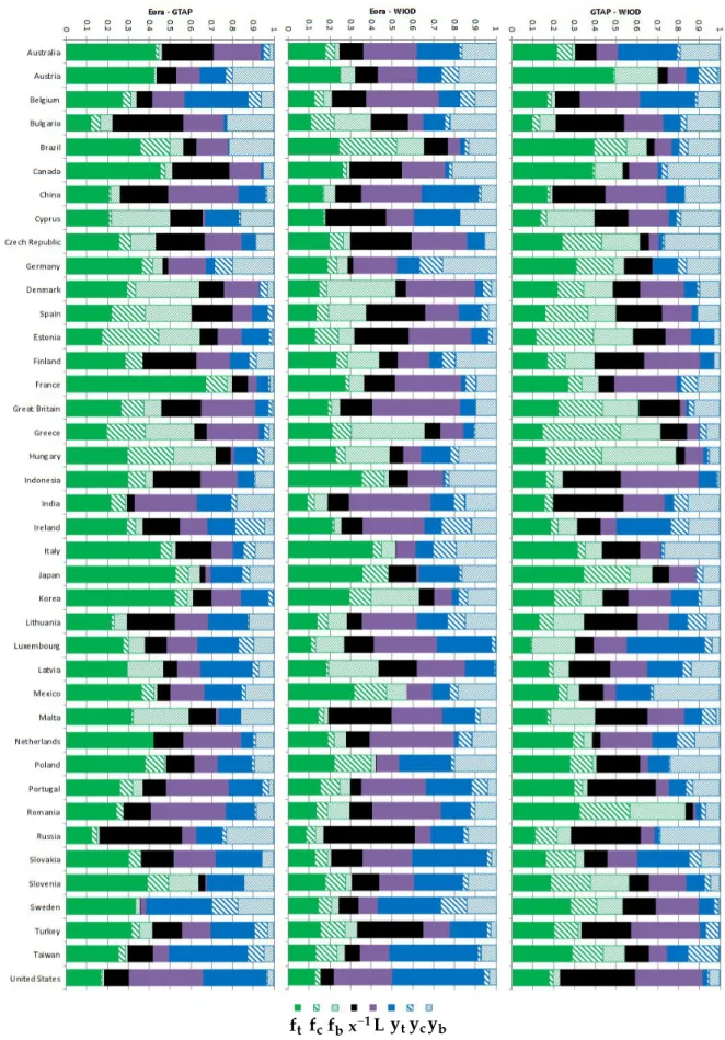
Figure 4: Relative contributions of SDA components to the variation in consumption-based CO2 emissions for individual countries as calculated by different pairs of MRIO database
The emissions total has most effect on the variation between Eora and GTAP although it is not quite as influential as the Leontief inverse (Table 8). One possible explanation is that Eora sources
emissions data from EDGAR and IEA, whereas GTAP only uses IEA (Table 1). The total final demand vector is important in the variation between Eora and GTAP and also Eora and WIOD but less so in the variation between GTAP and WIOD. For this last pairing, the basket of goods vector appears significant. GTAP and WIOD have quite different sectoral classifications with GTAP containing much more detail in the agricultural sectors. This might explain the difference in the basket of goods vector.
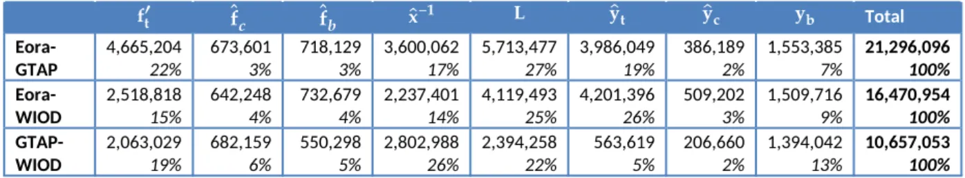
Table 8: Gross difference totals for the CC pairings
𝐟′𝐭 𝐟𝒄 𝐟𝒃 𝐱−𝟏 𝐋 𝐲𝐭 𝐲𝐜 𝐲𝐛 Total
Eora-GTAP 4,665,20422% 673,6013% 718,1293% 3,600,06217% 5,713,47727% 3,986,04919% 386,1892% 1,553,3857% 21,296,096100%
Eora-WIOD 2,518,81815% 642,2484% 732,6794% 2,237,40114% 4,119,49325% 4,201,39626% 509,2023% 1,509,7169% 16,470,954100%
4. Discussion
The aim of the study was to investigate why different MRIO databases produced different consumption-based CO2 emissions. A description of the different data sources, system structures and construction techniques employed in the Eora, GTAP and WIOD MRIO databases was provided and SDA was used to measure the relative contribution by each term of the Leontief equation towards MRIO outcome variation. An estimate of gross difference was also calculated. We form SDA equations using two terms and expand to detailed eight-term decompositions. This is one of the few MRIO SDA to calculate at this level of detail and to decompose emissions intensity. In addition, this work attempts to understand the uncertainty surrounding SDA calculations, including the non-uniqueness and dependency problems and we suggests novel techniques for calculating and presenting uncertainty findings.
Results show that the variation in the consumption-based CO2emissions measured by Eora, GTAP or WIOD can be explained largely by differences in total global emissions, differences in the Leontief inverse and differences in the total final demand vector. The share of the emissions by region and sector do not appear to contribute towards the variation, and neither does the share in final demand by region and product. The product share might be significant in the variation between GTAP and WIOD. Student’s t-tests suggest very high confidence in the calculation of the mean effect of the terms but we recognise the mean effect is just one of many solutions to the SDA and the range of possible outcomes needs to be considered carefully when drawing conclusions.
5. Conclusion
This study uses structural decomposition analysis to understand variation in MRIO outputs. The technique allows us to separate the influence of different parameters on the results, enabling investigation of how source data, system structure, technical coefficients and final demand contribute to variations in consumption-based emissions of countries as calculated by different MRIO databases. Although useful insights can be gained from this analysis, SDA alone cannot determine the exact cause of database variation; we are unable, for example to give the exact effect on the results on choosing EDGAR emissions data over IEA data or calculate the effect of a certain matrix balancing technique on the variation in consumption-based emissions.. We are also unable to comment on which is “the best” set of source data to use or matrix construction technique to follow because different data and system structures might be suitable for different applications. We suggest that SDA could be used alongside conventional uncertainty techniques, such as those demonstrated by Weber and Matthews (2007), Lenzen et al. (2010), Peters and Solli (2010), Peters et al. (2012) and Wilting, (2012), as a diagnostic tool and also as a way of presenting results. Such analyses helps to grow confidence in the application of MRIO if we are able to demonstrate that consideration has been given to variation in data and system build.
We recommend further studies which consider a wider range of MRIO databases and expand to additional years. Furthermore, while emissions and final demand have been decomposed to three further terms, the Leontief matrix remains a single entity and the effect of decisions in its construction remains undetermined here. For example, it would be interesting to consider whether differences in L are due to the domestic transactions or the imports to intermediate demand. We suggest building on the work of Wood and Lenzen (2009) and use structural path decomposition (SPD) to further explore the effects of differing Leontief matrices.
Acknowledgements
1. References
Andres, R. J., Boden, T. a., Bréon, F.-M., Ciais, P., Davis, S., Erickson, D., … Treanton, K. (2012). A synthesis of carbon dioxide emissions from fossil-fuel combustion. Biogeosciences, 9(5), 1845–1871. doi:10.5194/bg-9-1845-2012
Andrew, R. M. and Peters, G. P. (2013) A Multi-Region Input-Output Table based on the Global Trade Analysis Project Database (GTAP-MRIO). Economic Systems Research, 25(1), 99-121.
http://dx.doi.org/10.1080/09535314.2012.761953
Baiocchi, G. and Minx, J. C. (2010) Understanding Changes in the UK’s CO2 Emissions: A Global Perspective. Environmental Science & Technology, 44(4), 1177-1184.
http://dx.doi.org/10.1021/es902662h
Barrett, J., Peters, G., Wiedmann, T., Scott, K., Lenzen, M., Roelich, K., & Le Quéré, C. (2013). Consumption-based GHG emission accounting: a UK case study. Climate Policy, 13(4), 451–470. doi:10.1080/14693062.2013.788858
Bjerkholt, O., & Kurz, H. D. (2006). Introduction: the History of Input–Output Analysis, Leontief’s Path and Alternative Tracks. Economic Systems Research, 18(4), 331–333.
doi:10.1080/09535310601020850
Brizga, J., Feng, K., & Hubacek, K. (2014). Drivers of greenhouse gas emissions in the Baltic States: A structural decomposition analysis. Ecological Economics, 98, 22–28.
doi:10.1016/j.ecolecon.2013.12.001
CCC (2013) Reducing the UK's carbon footprint and managing competitiveness risks. The Committee on Climate Change, April 2013
Davis, S. J. and Caldeira, K. (2010) Consumption-based accounting of CO2 emissions. Proceedings of the National Academy of Sciences, 107(12), 5687-5692.
http://dx.doi.org/10.1073/pnas.0906974107
Davis, S. J., Peters, G. P. and Caldeira, K. (2011) The supply chain of CO2 emissions. Proceedings of the National Academy of Sciences, 108(45), 18554-18559.
http://dx.doi.org/10.1073/pnas.1107409108
Déqué, M., Rowell, D. P., Lüthi, D., Giorgi, F., Christensen, J. H., Rockel, B., … Hurk, B. (2007). An intercomparison of regional climate simulations for Europe: assessing uncertainties in model projections. Climatic Change, 81(S1), 53–70. doi:10.1007/s10584-006-9228-x
Dietzenbacher, E., Los, B., Stehrer, R., Timmer, M. and de Vries, G. (2013) The Construction of World Input-Output Tables in the WIOD Project. Economic Systems Research, 25(1), 71-98.
http://dx.doi.org/10.1080/09535314.2012.761180
Dietzenbacher, E. and Stage, J. (2006) Mixing oil and water? Using hybrid input-output tables in a Structural decomposition analysis. Economic Systems Research, 18(1), 85-95
http://dx.doi.org/10.1080/09535310500440803
Dietzenbacher, E., & Los, B. (1998). Structural Decomposition Techniques : Sense and Sensitivity. Economic Systems Research, 10(4), 307–323.
Dietzenbacher, E., & Los, B. (2000). Structural Decomposition Analyses with Dependent
Ewing, B. R., Hawkins, T. R., Wiedmann, T. O., Galli, A., Ertug Ercin, A., Weinzettel, J. and Steen-Olsen, K. (2012) Integrating ecological and water footprint accounting in a multi-regional input–output framework. Ecological Indicators, 23, 1-8.
http://dx.doi.org/10.1016/j.ecolind.2012.02.025
Feng, K., Chapagain, A., Suh, S., Pfister, S. and Hubacek, K. (2011) Comparison of bottom-up and top-down approaches to calculating the water footprints of nations. Economic Systems
Research, 23(4), 371-385. http://dx.doi.org/10.1080/09535314.2011.638276
Feng, K., Siu, Y. L., Guan, D. and Hubacek, K. (2012) Analyzing Drivers of Regional Carbon Dioxide Emissions for China. Journal of Industrial Ecology, 16(4), 600-611.
http://dx.doi.org/10.1111/j.1530-9290.2012.00494.x
Galli, A., Wiedmann, T., Ercin, E., Knoblauch, D., Ewing, B. and Giljum, S. (2012) Integrating
Ecological, Carbon and Water footprint into a “Footprint Family” of indicators: Definition and role in tracking human pressure on the planet. Ecological Indicators, 16, 100-112.
http://dx.doi.org/10.1016/j.ecolind.2011.06.017
Genty, A., Arto, I., & Neu. (2012). FINAL DATABASE OF ENVIRONMENTAL SATELLITE ACCOUNTS : TECHNICAL REPORT ON THEI COMMUNICATION. WIOD Deliverable, 4.6.
Guan, D., Hubacek, K., Weber, C. L., Peters, G. P. and Reiner, D. M. (2008) The drivers of Chinese CO2 emissions from 1980 to 2030. Global Environmental Change, 18(4), 626-634.
http://dx.doi.org/10.1016/j.gloenvcha.2008.08.001
Guan, D., Peters, G. P., Weber, C. L. and Hubacek, K. (2009) Journey to world top emitter: An analysis of the driving forces of China's recent CO2 emissions surge. Geophysical Research Letters, 36(L04709), 1-5. http://dx.doi.org/10.1029/2008GL036540
Hertwich, E. G. and Peters, G. P. (2009) Carbon Footprint of Nations: A Global, Trade-Linked Analysis. Environmental Science & Technology, 43(16), 6414–6420.
http://dx.doi.org/10.1021/es803496a
Hoekstra, R., & Bergh, J. J. C. J. M. Van Der. (2003). Comparing structural and index decomposition analysis. Energy Economics, 25, 39–64
Houghton, R. a., House, J. I., Pongratz, J., van der Werf, G. R., DeFries, R. S., Hansen, M. C., … Ramankutty, N. (2012). Carbon emissions from land use and land-cover change. Biogeosciences, 9(12), 5125–5142. doi:10.5194/bg-9-5125-2012
Jakob, M., & Marschinski, R. (2013). Interpreting trade-related CO2 emission transfers, 3(September 2012), 19–23. doi:10.1038/NCLIMATE1630
Lan, J., & Malik, A. (2013). Structural decompositional analysis of energy consumption in China and Russia – an application of the Eora MRIO databases. In J. Murray & M. Lenzen (Eds.), The Sustainability Practitioner’s Guide to Multi-Regional Input-Output Analysis (1st ed.). Champaign, Illinois, USA: Common Ground
Lee, H.-L. (2008) An Emissions Data Base for Integrated Assessment of Climate Change Policy Using GTAP, Global Trade Analysis Project, 2008.
Lenzen, M., Moran, D., Kanemoto, K. and Geschke, A. (2013) Building Eora: A Global Multi-Region Input-Output Database at High Country and Sector Resolution. Economic Systems Research, 25(1), 20-49. http://dx.doi.org/10.1080/09535314.2013.769938
Lenzen, M., Kanemoto, K., Moran, D., & Geschke, A. (2012a). Mapping the structure of the world economy. Environmental science & technology, 46(15), 8374–81. doi:10.1021/es300171x Lenzen, M., Moran, D., Kanemoto, K., Foran, B., Lobefaro, L., & Geschke, A. (2012b). International
trade drives biodiversity threats in developing nations. Nature, 486(7401), 109–112. doi:10.1038/nature11145
Lenzen, M., Wood, R., & Wiedmann, T. (2010). Uncertainty Analysis for Multi-Region Input–Output Models – a Case Study of the UK’s Carbon Footprint. Economic Systems Research, 22(1), 43–63. doi:10.1080/09535311003661226
Mélanie, J., Phillips, B. and Tormey, B. (1994) An international comparison of factors affecting carbon dioxide emissions. Australian Commodities, 1(4), 468-483.
Meng, B., Zhang, Y. and Inomata, S. (2013) Compilation and application of IDE-JETRO's international Input-Output tables. Economic Systems Research, 25(1), 122-142.
http://dx.doi.org/10.1080/09535314.2012.761597
Miller, R. E., & Blair, P. D. (2009). Input-output analysis : foundations and extensions. Cambridge University Press
Minx, J. C., Baiocchi, G., Peters, G. P., Weber, C. L., Guan, D. and Hubacek, K. (2011) A “Carbonizing Dragon”: China’s Fast Growing CO2 Emissions Revisited. Environmental Science &
Technology, 45(21), 9144-9153. http://dx.doi.org/10.1021/es201497m
Minx, J., Wiedmann, T., Wood, R., Peters, G. P., Lenzen, M., Owen, A., Scott, K., et al. (2009). Input – Output Analysis and Carbon Footprinting : an Overview of Applications. Economic Systems, 21(3), 187–216. doi:10.1080/09535310903541298
Moran, D. D., Lenzen, M., Kanemoto, K., & Geschke, A. (2013). Does Ecologically Unequal Exchange Occur? Ecological Economics, 89, 177–186. doi:10.1016/j.ecolecon.2013.02.013
Owen, A. (2013). Uncertainty and Variability in MRIO Analysis. In J. Murray & M. Lenzen (Eds.), The Sustainability Practitioner’s Guide to Multi-Regional Input-Output Analysis (1st ed.). Champaign, Illinois, USA: Common Ground.
Peters, G. P. (2007). Efficient Algorithms for Life Cycle Assessment, Input-Output Analysis, and Monte-Carlo Analysis. International Journal of LCA, 12(6), 373–380.
Peters, G. (2008) From Production-Based to Consumption-Based National Emission Inventories. Ecological Economics, 65(1), 13-23 http://dx.doi.org/10.1016/j.ecolecon.2007.10.014 Peters, G. P., Andrew, R. M., & Lennox, J. (2011). Constructing an Environmentally-Extended
Multi-Regional Input–Output Table Using the Gtap Database. Economic Systems Research, 23(2), 131–152. doi:10.1080/09535314.2011.563234
Peters, G. P., Guan, D., Hubacek, K., Minx, J. C. and Weber, C. L. (2010) Effects of China's Economic Growth. Science, 328(5980), 824-825. http://dx.doi.org/10.1126/science.328.5980.824-b Peters, G. P. and Hertwich, E. G. (2006) Structural analysis of international trade: Environmental
impacts of Norway. Economic Systems Research, 18(2), 155-181 http://dx.doi.org/10.1080/09535310600653008
Peters, G. P. and Hertwich, E. G. (2008a) CO2 Embodied in International Trade with Implications for Global Climate Policy Environmental Science & Technology, 42(5), 1401-1407.
http://dx.doi.org/10.1021/es072023k
Peters, G. P. and Hertwich, E. G. (2008b) Post-Kyoto greenhouse gas inventories: production versus consumption. Climatic Change, 86, 51-66. http://dx.doi.org/10.1007/s10584-007-9280-1 Peters, G. P., Weber, C. L., Guan, D. and Hubacek, K. (2007) Chinas growing CO2 emissions - a race
between increasing consumption and efficiency gains. Environmental Science & Technology, 41(7), 5939 -5944. http://dx.doi.org/10.1021/es070108f
Rose, A., & Casler, S. (1996). Input – Output Structural Decomposition Analysis : A Critical Appraisal A Critical Appraisal. Economic Systems, (January 2012), 37–41.
Rose, A., & Chen, C. Y. (1991). Sources of change in energy use in the U . S . economy , 1972-1982 analysis, 13, 1–21.
Sato, M. (2012). Embodied carbon in trade : a survey of the empirical literature. Centre for Climate Change Economics and Policy Working Paper No., (89).
Springmann, M. (2014). Integrating emissions transfers into policy-making. Nature Climate Change, 4(March), 177–181. doi:10.1038/NCLIMATE2102
Steen-Olsen, K., Owen, A., Hertwich, E.G. and Lenzen, M. (2014a) Effects of sectoral aggregation on CO2 multipliers in MRIO analyses.in press
Steen-Olsen, K., Owen, A., Barret, J., Guan, D., Hertwich, E.G., Lenzen, M. and Wiedmann, T. (2014b) Intercomparison of global multiregional input-output databases.in press
Steen-Olsen, K., Weinzettel, J., Cranston, G., Ercin, A. E. and Hertwich, E. G. (2012) Carbon, Land, and Water Footprint Accounts for the European Union: Consumption, Production, and
Displacements through International Trade. Environmental Science & Technology, 46(20), 10883-10891. http://dx.doi.org/10.1021/es301949t
Tian, X., Chang, M., Lin, C., & Tanikawa, H. (2014). China’s carbon footprint: A regional perspective on the effect of transitions in consumption and production patterns. Applied Energy, 123, 19–28. doi:10.1016/j.apenergy.2014.02.016
Tukker, A., de Koning, A., Wood, R., Hawkins, T., Lutter, S., Acosta, J., Rueda Cantuche, J. M., Bouwmeester, M., Oosterhaven, J., Drosdowski, T. and Kuenen, J. (2013) EXIOPOL – Development and Illustrative Analyses of a Detailed Global MR EE SUT/IOT. Economic Systems Research, 25(1), 50-70. http://dx.doi.org/10.1080/09535314.2012.761952 Tukker, A. and Dietzenbacher, E. (2013) Global Multiregional Input-Output Frameworks: An
Introduction and Outlook. Economic Systems Research, 25(1), 1-19. http://dx.doi.org/10.1080/09535314.2012.761179
Tukker, A., Poliakov, E., Heijungs, R., Hawkins, T. R., Neuwahl, F., Rueda-Cantuche, J. M., Giljum, S., et al. (2009). Towards a global multi-regional environmentally extended input–output database. Ecological Economics, 68(7), 1928–1937. doi:10.1016/j.ecolecon.2008.11.010 United Nations (1992) United Nations Framework Convention on Climate Change (UNFCCC).
FCCC/INFOR- MAL/84, GE.05-62220 (E) 200705. UNFCCC Secretariat, Bonn, Germany. http://unfccc.int/resource/ docs/convkp/conveng.pdf
Wachsmann, U., Wood, R., Lenzen, M., & Schaeffer, R. (2009). Structural decomposition of energy use in Brazil from 1970 to 1996. Applied Energy, 86(4), 578–587.
doi:10.1016/j.apenergy.2008.08.003
Weber, C. L. (2009) Measuring structural change and energy use: Decomposition of the US economy from 1997 to 2002. Energy Policy, 37(4), 1561-1570.
http://dx.doi.org/10.1016/j.enpol.2008.12.027
Weber, C. L. and Matthews, H. S. (2007) Embodied environmental emissions in U.S. international trade, 1997-2004. Environmental Science & Technology, 41(14), 4875-4881.
http://dx.doi.org/10.1021/es0629110
Weber, C. L., Peters, G. P., Guan, D. and Hubacek, K. (2008) The contribution of Chinese exports to climate change. Energy Policy, 36(9), 3572-3577.
http://dx.doi.org/10.1016/j.enpol.2008.06.009
Weinzettel, J., Hertwich, E. G., Peters, G. P., Steen-Olsen, K. and Galli, A. (2013) Affluence drives the global displacement of land use. Global Environmental Change, 23(2), 433-438.
http://dx.doi.org/10.1016/j.gloenvcha.2012.12.010
Weinzettel, J. and Kovanda, J. (2011) Structural Decomposition Analysis of Raw Material
Consumption - The Case of the Czech Republic. Journal of Industrial Ecology, 15(6), 893-907. http://dx.doi.org/10.1111/j.1530-9290.2011.00378.x
Wiedmann, T. (2009) A review of recent multi-region input-output models used for consumption-based emission and resource accounting. Ecological Economics, 69(2), 211-222.
http://dx.doi.org/10.1016/j.ecolecon.2009.08.026
Wiedmann, T. and Barrett, J. (2013) Policy-relevant Applications of Environmentally Extended MRIO Databases - Experiences from the UK. Economic Systems Research, 25(1), 143-156.
Wiedmann, T. O., Schandl, H., Lenzen, M., Moran, D., Suh, S., West, J., & Kanemoto, K. (2013). The material footprint of nations. Proceedings of the National Academy of Sciences of the United States of America, 1–6. doi:10.1073/pnas.1220362110
Wiedmann, T., Wilting, H. C., Lenzen, M., Lutter, S. and Palm, V. (2011) Quo Vadis MRIO?
Methodological, data and institutional requirements for multi-region input-output analysis. Ecological Economics, 70(11), 1937-1945. http://dx.doi.org/10.1016/j.ecolecon.2011.06.014 Wilting, H. C. (2012). Sensitivity and uncertainty analysis in MRIO modelling; some empirical results
with regard to the Dutch carbon footprint. Economic Systems Research, 24(2), 141–171. Wood, R. (2009). Structural decomposition analysis of Australia's greenhouse gas emissions. Energy
Policy, 37(11), 4943–4948. doi:10.1016/j.enpol.2009.06.060
Wood, R., & Lenzen, M. (2009). Structural path decomposition. Energy Economics, 31(3), 335–341. doi:10.1016/j.eneco.2008.11.003
Wood, R., Lenzen, M. and Foran, B. (2009) A Material History of Australia - Evolution of material intensity and drivers of change. Journal of Industrial Ecology, 13(6), 847-862.
http://dx.doi.org/10.1111/j.1530-9290.2009.00177.x
Yamakawa, A. and Peters, G. P. (2011) Structural decomposition analysis of greenhouse gas emissions in Norway 1990-2002. Economic Systems Research, 23(3), 303-318. http://dx.doi.org/10.1080/09535314.2010.549461
Zhang, H., & Lahr, M. L. (2014). China’s energy consumption change from 1987 to 2007: A multi-regional structural decomposition analysis. Energy Policy, 67, 682–693.
doi:10.1016/j.enpol.2013.11.069