Autoregressive Models and Non Local Self Similarity in Sparse Representation for Image Deblurring

(1)

International Journal of Innovative Technology and Exploring Engineering (IJITEE) ISSN: 2278-3075, Volume-8 Issue-9, July 2019



Abstract: Local area within a normal natural image can be thought as a stationary process. This can be modelled well using autoregressive models. In this paper, a set of autoregressive models will be learned from a collection of high quality image patches. Out of these models, one will be selected adaptively and will be used to regularize the input image patches. In addition to the autoregressive models, a non-local self-similarity condition was proposed. The autoregressive models will exploit local correlation of individual image, but a natural will have many repetitive structures. These structures, which are basically redundant, are very much useful in image deblurring. The performance of these schemes is verified by applying to image deblurring.

Index Terms: Autoregressive models, deblurring, non-local self-similarity, sparse domain selection.

I. INTRODUCTION

The natural images, generally, can be coded using structural primitives like edges and line fragments [1]. These fragments are similar to simple cell receptive fields [2]. Olshausen et al. proposed to use small number of basis functions which are chosen from an over-complete code set to represent natural image [3]. Recently, such kind of sparse coding schemes are extensively being studied to solve inverse problems. This is in proportion to the progress of l0-norm and l1-norm

minimization schemes [4].

Let

x



n is the signal to be encoded, and



1

,

2

,...,



n m m

 





 



is the assumed dictionary.

The sparse coding of x over



is to find a vector



1

;

2

;...;

m







 



such that

x







[5]. It is note that many coefficients in α are very close to zero. When the sparsity is measured as an l0-norm of α, which actually counts

the non-zero quantities in α, the problem of sparsity coding becomes . Here T is a number governing the amount of sparsity [6]. On the other hand, the vector α can be

found as





0 2

2

min

arg

ˆ











x







where λ is

an arbitrary constant. The l0-norm is non-convex, hence it is

many times replaced with l1-norm or weighted l1-norm, so that

the problem becomes convex [7, 8, 9, 4]. The most important part of sparse representation is the selection of dictionary



.

Revised Manuscript Received on July 05, 2019

Y Ravi Sankaraiah, Research Scholar, Dept. of ECE, JNTUK, Kakinada, India.

S. Varadarajan, Professor, Dept. of ECE, Sri Venkateswara University,

Many efforts are made in choosing the training image dataset and learning a dictionary [10-20, 6]. Let the training image

patches are grouped to form the set S,

. The objective of dictionary

learning is to optimize the dictionary



and the

representation coefficient matrix









₁

,...,



_N



so that

i i







s

.

This can be formulated using the following:

 

2

,

min

arg

ˆ

,

ˆ

F













S

Still the above minimization issue is non-convex. Different approaches were proposed to optimize the dictionary and coefficient matrix [11-13, 18-21]. Adaptive sparse domain selection (ASDS) scheme was presented in [22]. The scheme learns a series of compact sub-dictionaries and assigns adaptively each local patch a sub-dictionary as the sparse domain.

By learning a set of compact sub-dictionaries from high quality example image patches, the ASDS will perform the restoration. The example image patches are clustered into many clusters. Since each cluster consists of many patches with similar patterns, a compact sub-dictionary can be learned for each cluster. For an image patch to be coded, the best sub-dictionary that is most relevant to the given patch is selected. Since the given patch can be better represented by the adaptively selected sub-dictionary, the whole image can be more accurately reconstructed than using a universal dictionary, which will be validated by the experiments. With ASDS, a weighted l1-norm sparse representation model

will be proposed for restoration tasks. Suppose that {Φk},

k=1, 2… K, is a set of K orthonormal sub-dictionaries. Let x be an image vector, and xi=Rix, i = 1, 2… N, be the ith patch

(size: root (n) × root (n)) vector of x, where Ri is a matrix

extracting patch xi from x. With ASDS, the image restoration

problem can be modelled as:



1



2

min

arg

ˆ









y



DH



o



The design of Φk can be intuitively formulated by the

following objective function:







1



2

,

min

arg

ˆ

,

ˆ

k F k k k k k k

k





_

_

S















where Λk is the representation coefficient matrix of Sk over

Φk.

Autoregressive Models and Non-Local Self

Similarity in Sparse Representation for Image

Deblurring

(2)

II. AUTOREGRESSIVEMODELS

As described in previous section, the training data set was divided into K sub-datasets SK. One autoregressive model can be trained for each SKby utilizing all the patches in it. Assume that the support of the autoregressive model is a square window, and the projected autoregressive model will estimate the middle pixel in the square with the knowledge of its neighbor pixels which are the boundary pixels of the square window. Determination of size window is very difficult. A high order of the window will result in data over-fitting. In this paper, a window size of 3x3 is used. So, the total number of pixels becomes 9, and the number of neighbors of middle pixel is 8, which is the order of the autoregressive model. The vector of autoregressive model arKof one of the sub-dataset SK can be obtained using the solution of the least square problem given below.













K S

q

a

i s i T i a

s

2

K

arg

min

r

‘si’ is the middle pixel of the image patch Si and qi is the

vector with all its neighbors. When this training process is applied to all the sub-dataset, a set of autoregressive models {ar1, ar2,..., arK}. This set of autoregressive models will be used for regularization. In the previous section, selection of sub-dictionaries was presented. Similar to that, the selection of autoregressive models will be done. Using the estimate

x

ˆ

,

the high pass filtered version

x

ˆ

_ih can be calculated. Now,

assume

2

ˆ

arg min

h

i k c i c k

k





x

 



, and the

autoregressive model arkito be assigned to the image patch xi. The vector holding the holding the neighbors of xi is denoted

by



_i. Now, the prediction error of xi using arki and



i

should be minimum. In other words the term 2

2

i

T

i K i

x



ar XY

need to be optimized to be smallest.

Incorporating this condition on the sparse representation, the objective function will look like the following.

2

, , 2

1 1

ˆ arg min | |

i i

N N

T i j i j i k i

i j x

y DH x

                        







X 

ar

Here,



balances the effect of autoregressive regulating

term.

III. NON-LOCALSIMILARITY

Adaptive regularization based on autoregressive model feats the local features in each and every image patch. In addition to the local features, many repetitive patterns are present on any natural image. These non-local redundancy is very much helpful in further improvement of quality of reconstructed images. For each local patch xi, similar patches in the image need to be identified. A patch

X

l_i is said to be

similar patch if

2

ˆ

l l

i i i

e



X



X



t

. Here t is a threshold.

Assume xi and

l i

x

to be middle pixels of the patches

X

_i and

l i

X

respectively.

Now use the weighted average of

x

_il, 1 L l l i i l

b x





can be used

to estimate xi. Here the weight given to

l i

x

is fixed using the

relation _il

1 exp



l_i

/



i

b

e h

c





. Here h is governing factor of

weight and ci is the normalizing factor given

by





1

exp

/

L l i i l

c

e

h







. The estimate error

2

1 ₂

L l l

i i i

i

x

b x







can be rewritten as

2

T l i i i

x



b



, where bi

is the column vector containing all the weights

b

_il and



_i is

the column vector that holds all

x

_il. After incorporating the

non-local similarity regularization into sparse representation, we get the following.

2 2

, ,

2 2

1 1

ˆ arg min N N T

i j i j i i i i j

y DH o x b

                   





 .

IV. RESULTSANDDISCUSSIONS

In this work, to learn dictionaries and thereby sub-dictionaries, two sets of high quality test images were considered. From each set on dictionary and corresponding sub dictionaries are formed. The selection of test images for learning the dictionary is so critical. The test images should have all the possible patterns to represent the features that are there in input images. The effect of the selection of these high quality images is presented in this section. Two kinds of blurs are considered, uniform and Gaussian blurs. Uniform blur is created by convolving the original image with a kernel of specific order. In the experiments two sizes are considered, 3x3 and 9x9. When the dimension of the kernel is more, the effect of the blur will also be more. So, the effect of kernel of 9x9 will be more than that with a kernel of 3x3. Gaussian blur is also applied in two varieties, one with standard deviation of 1 and another with 3. The effect of Gaussian blur with the standard deviation of 3 is predominant than the other. The procedure is an iterative process, and it is iterated for 1000 times. For each 40 iterations, the peak signal to noise ratios is noted. Fig.1.

(3)

Input Image

Uniform blur with kernel of 3x3 size PSNR = 30.713 dB

Uniform blur with kernel of 9x9 size PSNR = 23.871 dB

Gaussian blur with standard deviation of 1 PSNR = 30.155 dB

Gaussian blur with standard deviation of 3 PSNR = 24.072 dB

(4)

[image:4.595.80.516.60.376.2]

Table 1. Simulation results on Uniform blur with 3x3 kernel

Dictionary – 1 Dictionary – 2

It ASDS ASDS

Autoregressive

ASDS Autoregressive

with non-local similarity

ASDS ASDS

Autoregressive

0 30.714 30.714 30.714 30.714 30.714 30.714

80 35.375 35.759 36.587 35.381 35.758 36.591

160 35.117 35.690 36.663 35.132 35.697 36.672

240 35.043 35.685 36.679 35.061 35.692 36.681

320 34.999 35.748 36.631 35.021 35.743 36.621

400 34.979 35.801 36.596 34.999 35.790 36.584

480 34.966 35.808 36.595 34.984 35.794 36.584

560 34.956 35.808 36.594 34.970 35.794 36.585

640 34.950 35.797 36.571 34.962 35.789 36.567

720 34.945 35.791 36.563 34.957 35.785 36.561

800 37.089 38.053 38.606 37.096 38.024 38.603

880 37.232 38.106 38.625 37.231 38.076 38.626

960 38.036 38.568 38.787 38.037 38.540 38.778

1000 38.030 38.570 38.790 38.040 38.540 38.780

[image:4.595.79.517.326.697.2]

SSIM 0.965 0.967 0.968 0.965 0.967 0.968

Table 2. Simulation results on Uniform blur with kernel of 9x9

Dictionary - 1 Dictionary – 2

Autoregressive

ASDS ASDS

Autoregressive

0 23.871 23.871 23.871 23.871 23.871 23.871

80 28.625 28.611 28.620 28.619 28.604 28.614

160 29.316 29.282 29.157 29.310 29.272 29.151

240 29.839 29.767 29.444 29.835 29.757 29.438

320 30.152 30.068 29.822 30.144 30.056 29.816

400 30.361 30.304 30.330 30.353 30.293 30.317

480 30.505 30.459 30.563 30.501 30.454 30.554

560 30.607 30.562 30.685 30.605 30.565 30.688

640 30.684 30.639 30.846 30.679 30.644 30.857

720 30.739 30.695 30.985 30.733 30.701 30.994

800 31.124 31.019 31.160 31.111 31.019 31.166

880 31.260 31.144 31.241 31.236 31.137 31.247

960 31.242 31.126 31.187 31.204 31.103 31.189

1000 31.270 31.150 31.200 31.230 31.130 31.200

(5)

[image:5.595.78.518.76.383.2]

Table 3. Simulation results on Gaussian blur with standard deviation of 1

Autoregressive

ASDS ASDS

Autoregressive

0 30.155 30.155 30.155 30.155 30.155 30.155

80 36.061 35.852 34.167 36.045 35.856 34.186

160 36.049 35.820 32.908 36.030 35.827 32.936

240 36.073 35.831 32.174 36.056 35.833 32.206

320 36.033 35.660 31.680 36.020 35.664 31.712

400 35.968 35.387 31.333 35.967 35.402 31.364

480 35.950 35.320 31.079 35.955 35.339 31.111

560 35.943 35.297 30.888 35.950 35.318 30.922

640 35.935 35.177 30.743 35.943 35.202 30.778

720 35.931 35.088 30.629 35.938 35.119 30.666

800 37.519 36.353 30.511 37.474 36.391 30.562

880 37.593 36.585 30.372 37.534 36.613 30.436

960 37.886 37.368 30.260 37.827 37.347 30.342

1000 37.890 37.390 30.200 37.830 37.370 30.290

SSIM 0.965 0.953 0.721 0.965 0.953 0.726

Table 4. Simulation results on Gaussian blur with standard deviation of 3

Autoregressive

ASDS ASDS

Autoregressive

0 24.072 24.072 24.072 24.072 24.072 24.072

80 26.840 26.824 26.834 26.838 26.821 26.834

160 27.149 27.087 27.122 27.145 27.084 27.123

240 27.351 27.233 27.305 27.341 27.234 27.310

320 27.478 27.369 27.432 27.465 27.370 27.435

400 27.581 27.516 27.529 27.566 27.517 27.532

480 27.652 27.610 27.607 27.639 27.604 27.610

560 27.702 27.676 27.671 27.691 27.667 27.674

640 27.742 27.742 27.723 27.733 27.733 27.725

720 27.773 27.802 27.768 27.766 27.792 27.765

800 27.795 27.873 27.880 27.781 27.853 27.871

880 27.825 27.913 27.930 27.801 27.882 27.917

960 27.835 27.940 27.966 27.800 27.898 27.949

1000 27.840 27.950 27.980 27.810 27.910 27.960

SSIM 0.863 0.868 0.868 0.862 0.867 0.867

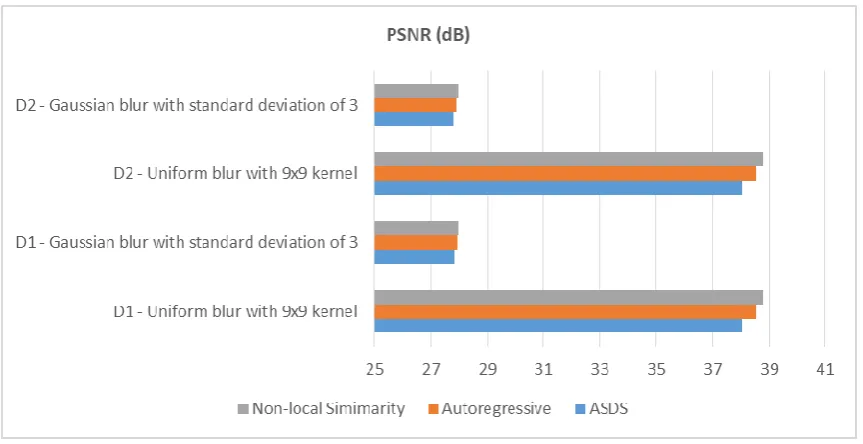
The effect of autoregressive model and extracting non-local similarity is apparent when the blurring is predominant. Hence, the effect can well be observed in

[image:5.595.77.536.419.761.2]

(6)

[image:6.595.83.515.48.270.2]

Fig. 2 PSNR values obtained with different techniques when blurring is more

V.CONCLUSIONS

In this paper, sparse representation is proposed with few improvement terms and applied on image deblurring. Uniform and Gaussian blurs are simulated and deblurring was done using sparse representation based schemes. Adaptive selection of sub-dictionaries was presented. In addition to the proposal of the said sparse representation, to characterize local image structures, autoregressive models are proposed. These autoregressive models pre-learned from training dataset. Out of the all autoregressive models learned, one or few models will be adaptively chosen to regularize the solution space. Along with the autoregressive models, a non-local self-similarity condition was also proposed. A natural image will have several repetitive image structures. These conditions help in preserving the sharp edges. The simulation results proved the superiority of the two improvements proposed, specifically when the blurring quantity is more.

REFERENCES

1. D. Field, “What is the goal of sensory coding?” Neural Computation,

vol. 6, pp. 559-601, 1994.

2. B. Olshausen and D. Field, “Emergence of simple-cell receptive field properties by learning a sparse code for natural images,” Nature, vol. 381, pp. 607-609, 1996.

3. B. Olshausen and D. Field, “Sparse coding with an overcomplete basis set: a strategy employed by V1?” Vision Research, vol. 37, pp. 3311-3325, 1997.

4. J. A. Tropp and S. J. Wright, “Computational methods for sparse solution of linear inverse problems,” Proceedings of IEEE, Special Issue on Applications of Compressive Sensing & Sparse Representation, vol. 98, no. 6, pp. 948-958, June, 2010.

5. S. Chen, D. Donoho, and M. Saunders, “Atomic decompositions by basis pursuit,” SIAM Review, vol. 43, pp. 129-159, 2001.

6. A. M. Bruckstein, D. L. Donoho, and M. Elad, “From sparse solutions of systems of equations to sparse modeling of signals and images,” SIAM Review, vol. 51, no. 1, pp. 34-81, Feb. 2009.

7. E. Candès and T. Tao, “Near optimal signal recovery from random projections: Universal encoding strategies?” IEEE Trans. on Information Theory, vol. 52, no. 12, pp. 5406 - 5425, December 2006. 8. E. J. Candes, “Compressive sampling,” in Proc. of the International

Congress of Mathematicians, Madrid, Spain, Aug. 2006.

9. E. Candes, M. B. Wakin, and S. P. Boyd, “Enhancing sparsity by reweighted l1 minimization,” Journal of Fourier Analysis and Applications, vol. 14, pp. 877-905, Dec. 2008.

10. M. Elad, M.A.T. Figueiredo, and Y. Ma, “On the Role of Sparse and Redundant Representations in Image Processing,” Proceedings of IEEE, Special Issue on Applications of Compressive Sensing & Sparse Representation, June 2010.

11. J. Mairal, M. Elad, and G. Sapiro, “Sparse Representation for Color Image Restoration,” IEEE Trans. on Image Processing, vol. 17, no. 1, pages 53-69, Jan. 2008.

12. J. Mairal, F. Bach, J. Ponce, G. Sapiro and A. Zisserman, “Non-Local Sparse Models for Image Restoration,” International Conference on Computer Vision, Tokyo, Japan, 2009.

13. M. Aharon, M. Elad, and A. Bruckstein, “K-SVD: an algorithm for designing overcomplete dictionaries for sparse representation,” IEEE Trans. Signal Process., vol. 54, no. 11, pp. 4311-4322, Nov. 2006. 14. J. Mairal, G. Sapiro, and M. Elad, “Learning Multiscale Sparse

Representations for Image and Video Restoration,” SIAM Multiscale Modeling and Simulation, vol. 7, no. 1, pages 214-241, April 2008. 15. R. Rubinstein, M. Zibulevsky, and M. Elad, “Double sparsity: Learning

Sparse Dictionaries for Sparse Signal Approximation,” IEEE Trans. Signal Processing, vol. 58, no. 3, pp. 1553-1564, March 2010. 16. Jaya Krishna Sunkara, Kuruma Purnima, Suresh Muchakala,

Ravisankariah Y, “Super-Resolution Based Image Reconstruction”, International Journal of Computer Science and Technology, vol. 2, Issue 3, pp. 272-281, September 2011.

17. G. Monaci and P. Vanderqheynst, “Learning structured dictionaries for image representation,” in Proc. IEEE Int. conf. Image Process., pp. 2351-2354, Oct. 2004.

18. Jaya Krishna Sunkara, Sundeep Eswarawaka, Kiranmai Darisi, Santhi Dara, Pushpa Kumar Dasari, Prudhviraj Dara, “Intensity Non-uniformity Correction for Image Segmentation”, IOSR Journal of

VLSI and Signal Processing (e-ISSN: 2319-4200, p-ISSN: 2319-4197), Volume 1, Issue 5, PP 49-57, Jan. -Feb 2013.

19. Jaya Krishna Sunkara, Uday Kumar Panta, Nagarjuna Pemmasani, Chandra Sekhar Paricherla, Pramadeesa Pattasani, Venkataiah Pattem, “Region Based Active Contour Model for Intensity Non-uniformity Correction for Image Segmentation”, International Journal of Engineering Research and Technology (RIP) (p-ISSN: 0974-3154) , Volume 6, Number 1, pp. 61-73, 2013.

20. R. Rubinstein, A.M. Bruckstein, and M. Elad, “Dictionaries for sparse representation modeling,” Proceedings of IEEE, Special Issue on Applications of Compressive Sensing & Sparse Representation, vol. 98, no. 6, pp. 1045-1057, June, 2010.

21. K. Engan, S. Aase, and J. Husoy, “Multi-frame compression: theory and design,” Signal Processing, vol. 80, no. 10, pp. 2121-2140, Oct. 2000. 22. Y. Ravi Sankaraiah and S. Varadarajan, “Dictionary Learning Based

(7)

AUTHORSPROFILE

Y. Ravi Sankaraiah received B.Tech in Electronics and Communication Engineering from KSRMCE, Kadapa in 1998 and M.Tech in Applied Electronics from Sathyabama University, Chennai in 2007. He worked as Network Engineer in Optonet Technologies Pvt. Ltd., Hyderabad, and HOD, Department of Electronics and Communication Engineering at Priyadarshini College of Engineering, Sullurpet. Currently he is working as HOD, Department of ECE, Bheema Institute of Technology and Science, Adoni and pursuing his Ph.D on Image deblurring at JNTUK, Kakinada.