Abstract: ALB is commonly known as combinatorial optimization problem in manufacturing industries and operation management circumstances. Because of the NP-hard characteristics of ALB problem, lot of tries have been done to solve the problem professionally. The critical concern in analysing ALB is how to generate a possible task order which does not disrupt the priority restrictions. This job arranging is a vigorous work to be answered prior to passing on jobs to workstation. Balance delay time (total idle time) is the total of idle time on fabrication assembly lines triggered by the irregular partition of work among operators or stations. In this thesis, SALBP-1 analysed using the three heuristic techniques. Kilbridge and Westers Method (KWM), Ranked Positional weight (RPW) and biologically inspired evolutionary computing tool which is heuristic treated Genetic Algorithm (GA) was applied to solve the ALB problem with the main aim of reducing the balance delay time in the workstation and the best method was selected. The selection criterion was based on the minimum balance delay for the sample problem. The result obtained by heuristic treated GA with 4.545% of balance delay for the sample problem taken was the best when compared to other two methods.
Keywords: Assembly line, Balance delay time, Genetic Algorithm (GA), Heuristic algorithms
I.INTRODUCTION:
1.1. Assembly Line: Assembly line is an order of production equipment called workstations, which are connected together by a kind of material-handling system. In general, to measure Assembly line we have two methods. The first one is technical measurements such as cycle time, balance delay or total idle time, and minimizing the number of workstations. The second one is economic measurements like profit maximization and cost minimization. violating assignment restrictions based on the objective such as reducing the overall cost, cycle time, number of workstations, maximizing throughput, efficiency, etc. (Baybars,1986). [1]
1.3 Simple Assembly Line Balancing Problem: simple assembly line problem (SALBP) which contain the following characteristics: -
Task time is assumed to be deterministic Serial and paced assembly line is considered etc.
Revised Manuscript Received on July 10, 2019.
Habtamu Mitiku Feyissa, College of Engineering Research and Technology Transfer Coordinator, Department of Mechanical Engineering, Maddawalabu University, Bale Robe, Ethiopia-247
A Indra Reddy, Assistant Professor, Mechanical Department, Koneru Lakshmaiah Education Foundation, Vaddeswaram, A.P.
Yakkala. M.K Raghunadh, Assistant Professor, Mechanical Engineeri- -ng, Department, Guru Nanak Institutions Technical Campus, Hyderabad 501516.
Figure: 1. General Motors Auto Assembly Line [2]
1.4 Objectives of the Project:
The objectives that must be achieved in the project are:- a.To optimize balance delay time in assembly line for the benchmark problems taken.
b.To find out better Heuristic algorithm for the sample problems analysed.
First of all, it is crucial to have a complete list of operations of the assembly line and their times, because this data is the basic reason for a line to exist, and evaluation of the balance of a line cannot be made without this data.
II. LITERATURE REVIEW
The overall exercise in the ALB is to allocate works to workstations in such a way that each total time of allocated works to each workstation has an equivalent cycle time. Bryton defined and studied SALBP as early as 1954.[3] In the following year (1955), Boysen, Fliedner, & Scholl, 2007, 2008[4]; Erel&Sarin, 1998; Ghosh & Gagnon, 1989; Scholl & Becker, 2005, 2006; [5] During subsequent years, SALBP became a popular topic. Kim, Kim, and Kim (1996) divided SALBP into five kinds of problems, of which type I problem (SALBP-1) and type II problem (SALBP- 2) are the two basic optimization problems.[6]
Researchers have published many studies on the solution for the SALBP-1 problem. Hackman [7], Magazine, and Betts and Mahmoud (1989)[8], , and Ozdemirel (2009) have suggested BB methods for application. Chica, Cordon, and Damas (2011) [9] developed a model that involves the joint optimization of conflicting objectives such as the cycle time, the number of stations, and/or the area of these stations.
Analysis of delay time and layout using
Heuristics algorithms
III.METHODOLOGY
This chapter presents in detail the kind of problems investigate during this project. It also explains the algorithms that are going to be used to solve the problems
The aim is to get the finest balance for that type of line. To answer the difficulty the algorithms used are heuristic methods.
3.1 Designing Product Layouts-Line balancing
A product layout consists of several processes arranged. This is significant because all of items follow virtually (almost) the same order of operations.
Steps in Solving Line Balancing Problems The steps in line balancing are as follows:- A) Draw precedence diagram
B) Determine the cycle time for the line C) Assign tasks to workstations D) Calculate the efficiency of the line 3.2 Algorithms Proposed in This Study
[image:2.595.352.500.52.303.2]In this section, there are presented some algorithms that are used to solve the SALP-1 problem. These algorithms aim to reduce the No of stations in the line, with a fixed cycle time.
Fig.2.General Scheme of Evolutionary Process. 3.2.1.1Working principle of Genetic Algorithm
Genetic algorithm begins with several solutions (represented by chromosomes) called population. Solutions from one population are taken and used to form a new population. This is motivated by the possibility that a new population will be better than the old one. Solutions are identified bestowing to their ability to form new offspring. This repeated until some condition is satisfied.
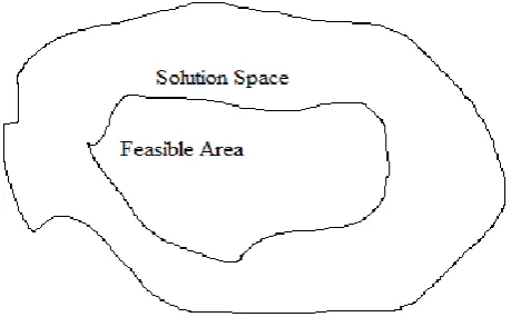
[image:2.595.69.267.327.413.2]Fig. 3. Search Space/State Space
Fig.4 Genetic Algorithm Program Flow Chart According to Darwin’s theory of evolution “survival of the fittest” – the fittest ones should continue and give new offspring.
IV. CASE STUDY 4.1 Study of a SMAL
The assembly line design [10] should account for the Production Rate Rp that is sufficient to reach the desired demand (Quantity) for the product. The product volume is often determined as an annual quantity as follow:
Q = Rp= Da/50SwHsh (4.1) Where Sw = number of shifts per week, Da = annual quantity, 50 = number of weeks per year, Hsh = hr/shift. Supposing the company operates 50 wk/yr. This feature must change to a cycle time Ct which determines the line time interval
Ct = 60*E / Rp (4.2)
The cycle time C
testablishes the ideal cycle rate for
the line RC
Rc = 60 / Ct (4.3)
Line Efficiency E is then calculated as:
E = (Rp / Rc) = (Ct / Tp) (4.4)
An assembled product requires a certain total amount of time to build, called the Work Content Time Twc. Number of workers usually determined on the production line as:
W = WL / AT (4.5) The repositioning efficiency (Er) is:
Total system time at particular station jTsj = C – Tr (4.6)
Repositioning Efficiency Er = Ts / C = (C – Tr) / C (4.7)
4.2 Data Collection
In this section the proposed algorithms are applied to solve
[image:2.595.53.283.550.697.2]http://www.assembly-line-balancing.de. one sample problem is selected for analysis. It is 21 parts, with 21seconds. Table below gives a list of the number of tasks, task times and precedence relations for the cycle time of 21seconds.
Table 1. Work Parts Going To Be Assigned To the Stations Work Parts Task times Tei
(Seconds)
Preceded by
1 4 -
2 3 1
3 9 1
4 5 3
5 9 4
6 4 5
7 8 5
8 7 6
9 5 8
10 1 9
11 3 9
12 1 9
13 5 9
14 3 7
15 5 10,11,12
16 3 15
17 13 13,16
18 5 13,15
19 2 14,18
20 3 17
21 7 2,4
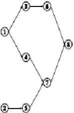
Fig.5. The proposed precedence diagram which has 21 tasks
4.3 Data Analysis
4.3.1 Kilbridge and Wester Column Method (KWM)
Problem (n=21tasks)
Work parts in this method are selected for assignment to workstations according to their position in the precedence diagram, Tables.2 and.3. Therefore, work parts were arranged
into columns, Figure 6, and then organized into a list according to their column, with the parts in the first column listed first. Table 3 shows a list of parts of the column method,
starting with the highest value of the time for each column. The advantage of this method is that a given part could be set
in over one column. For example, all of the columns for that
[image:3.595.69.271.107.543.2]stations as possible until all parts have been assigned as shown in the priority diagram, Fig. 6.
Fig. 6. Work Parts Arranged into Columns for the Kilbridge and Wester Method
Table.2 Work Parts Assigned as Stations According to the Column Method
Work parts
column Tei (sec.)
Preceded by
1 A 4 -
2 B&C 3 1
3 B 9 1
4 C 5 3
5 D 9 4
6 E 4 5
7 E-G 8 5
8 F 7 6
9 G 5 8
10 H 1 9
11 H 3 9
12 H 1 9
13 H-J 5 9
14 H-K 3 7
15 I&J 5 10,11,12
16 J 3 15
17 K 13 13,16
18 K 5 13,15
19 L 2 14,18
20 L 3 17
[image:3.595.334.517.230.501.2]21 D 7 2,4
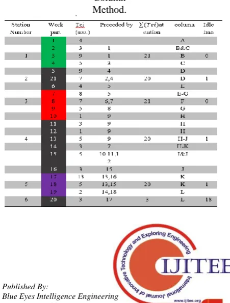
Table 3 Work Parts Arranged According to Tei Values for the Column
[image:3.595.327.523.240.634.2] [image:3.595.319.545.527.825.2]Fig. 7 Configuration Layouts for Assembly Line Following KWM
Idle time of workstation1=0 Idle time of workstation2=1sec. Idle time of workstation3=0 Idle time workstation4=1sec. Idle time of workstation5=1sec. Idle time of workstation6=18sec.
Total idle time=Balance delay
time= =21seconds
%Delay=( )*100%
Where, n is number of station, C is cycle time and Twc is total
work content time.
From this the percentage of balance delay is 16.667% 4.3.2 Ranked Positional Weight Method (RPW) By RPW method the calculated result is shown as follows in table 4. bellow.
Table 4. Work Parts Assigned as Stations bestowing to the RPW
Work parts Tei (sec.)
RPW
1 4 105
2 3 10
3 9 98
4 5 89
5 9 77
6 4 57
7 8 64
8 7 53
9 5 46
10 1 32
11 3 34
12 1 32
13 5 28
14 3 5
15 5 31
16 3 19
17 13 16
18 5 7
19 2 2
20 3 3
[image:4.595.50.261.51.134.2]21 7 7
[image:4.595.308.543.80.431.2]Table 5 Work Parts Arranged According to Tei Values for the RPW.
Fig. 8. Schematic Diagram Showing the Distribution of Station Along a Straight Line Following RPW. From the table above:-
Idle time of workstation1 = 0 Idle time of workstation2 =0 Idle time of workstation3 =1sec. Idle time of workstation4 =1sec. Idle time of workstation5=1sec. Idle time of workstation6=18sec.
Total idle time= Balance Delay Time = =21seconds
4.3.3 Genetic Algorithm
A) Chromosome Representation and Initial population Four heuristic algorithms and a version of topological sorting are used to generate initial population. The four heuristics used are KWM, RPW, Longest processing time and maximum task followers.
Fig. 9 Sample Precedence Network
Table .6 Example of Encoding Method
Iteration Available
set
Random selection
Append to string
1 {1,2} 1 (1)
2 {2,3,4} 4 (1 4)
3 {2,3} 2 (1 4 2)
4 {3,5} 5 (1 4 2 5)
5 {3,7} 3 (1 4 2 5 3)
6 {6,7} 7 (1 4 2 5 3 7)
7 {6} 6 (1 4 2 5 3 7 6)
8 {8} 8 (1 4 2 5 7 6 8)
B) Repair process
The Table 7 shows the step-by-step results of the repair method. An example of infeasible offspring (2 7 1 4 5 3 6 8) is shown here below.
Table.7 Example of Repair Method Iteration Available
set
Infeasible offspring
Repaired string 1 {1,2} (1 7 2 4 5 3 6
8)
(1) 2 {2,3,4} (1 7 2 4 5 3 6
8)
(1 2) 3 {3,4,5} (17 2 453 6 8) (1 2 4) 4 {3,5} (17 2 4 53 6 8) (1 2 4 3) 5 {5,6} (17 2 4 5 3 6 8) (1 2 4 3 5) 6 {6,7} (17 2 4 5 3 6 8) (1 2 4 3 5 6)
7 {7} (17 2 4 5 3 6 8)
(1 2 4 3 5 6 7) 8 {8} (17 2 4 5 3 6
8)
(1 2 4 3 5 6 7 8)
9 {} (1 2 4 3 5 6 7
8) C) Fitness Evaluation Function
Fitness evaluation is to check by subject to precedence constraint.
Where
C is cycle time,
Tj (j=1...mstar) is operation time of workstation j and m star is total number of workstations.
For example: p1 = [a b c d e f g h]
p2 = [1 2 3 4 5 6 7 8] random crossover point = 3 Child1 = [a b c 4 5 6 7 8]
Child2= [1 2 3 d e f g h]
Station oriented algorithm for finding a solution to ALBP for j := 1 to M do (assign tasks on workstation)
Identify available tasks, A, whose predecessors have been assigned
Determine from available tasks, Afit={i|∀i∈ A:ti≤ sj} Choose a task i∈Afit by some heuristic.
if Afit =ø then break &then proceed to the next workstation if all tasks are assigned then return ALBP sequence using m := j workstations.
In this study, code is written using Matlab software R2010b.TheMatlab program which used heuristics methods to solve the problems. The two heuristics chosen are the max following and longest task time methods. The max following method works in the way that it chooses the task which is the precedence for the most tasks, that is, it has the most tasks that can’t be started until it has been completed. The longest task time method chooses the task which has the longest task time. 4.3.3.1Mathematical Model
Notations used:-
n number of tasks on the assembly line m number of workstations in the assembly line M maximum number of workstations
P immediate precedence matrix of dimension n × n,
P (i, j) = 1 if task j is an immediate successor of task i, 0 otherwise.
F immediate followers matrix of dimension n× n,
F (i, j) = 1 if task j is an immediate follower of task i, 0 otherwise.
C cycle time of the assembly line ti operation time of task i
sj the slacktime for the j-th workstation
Xij= 1 if task i is assigned to workstation j, otherwise 0
yj =1 if workstation j, 0 < k M has a task assigned to it, otherwise 0
Mmin Theoretical minimum number of workstations, Mmin=
4.3.3.2Model
A model for SALBP-1, utilizing the notations presented is as follows:
Objective function
Minimize (4.8)
Where,
is total idle time, C is cycle time,
Tj (j=1...mstar) is operation time of workstation j mstar is total number of workstations.
Constraints
(4.9)
(4.11)
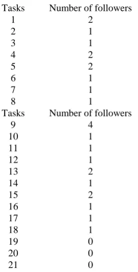
[image:6.595.313.540.106.483.2]The objective function (4.8) consists in minimizing the total idle time of the assembly line. Constraint (4.9) guarantees that every task i is assigned to one and only one workstation. Constraint (4.10) ensures that the summation of time of the tasks assigned to workstation j does not exceed cycle time. Constraint (4.11) imposes the precedence constraints. Table 8 Lists of Tasks According to Number of Followers for
Task Number 21 Tasks Number of followers
1 2
2 1
3 1
4 2
5 2
6 1
7 1
8 1
Tasks Number of followers
9 4
10 1
11 1
12 1
13 2
14 1
15 2
16 1
17 1
18 1
19 0
20 0
21 0
Table 9 Lists of Tasks According to Descending Order of Followers for Task Number 21
Tasks Number of followers in descending order
9 4
1 2
4 2
5 2
13 2
Tasks Number of followers in descending order
15 2
2 1
3 1
6 1
7 1
8 1
10 1
11 1
12 1
14 1
16 1
17 1
18 1
19 0
20 0
21 0
[image:6.595.100.239.180.454.2]Table 10 Work Parts Arranged According to Tei Values for the Maximum Followers of Tasks After Running on Gatoolbox.
Fig. 10. Configuration Layouts for Assembly Line Following Maximum Follower.
Balance delay time (total idle time) =21seconds
Table 11 Lists of Tasks According to Descending Order of Work Parts Time
Work parts
Work parts time Tei (sec.) in descending order
17 13
3 9
5 9
7 8
8 7
21 7
4 5
9 5
13 5
15 5
18 5
1 4
6 4
2 3
[image:6.595.83.255.485.779.2]14 3
16 3
20 3
19 2
10 1
[image:7.595.309.530.50.138.2]12 1
Table 12 Work Parts Arranged According to Tei Values for the Largest Task Time After Running On Matlab Gatoolbox.
Fig.11 Configuration Layouts for Assembly Line Longest Time Task.
Balance delay time (total idle time) =21seconds.
[image:7.595.104.200.51.120.2]After analyzing the tasks’ sequences using the above four heuristics the crossover and mutation program has been written as follows on matlab software.
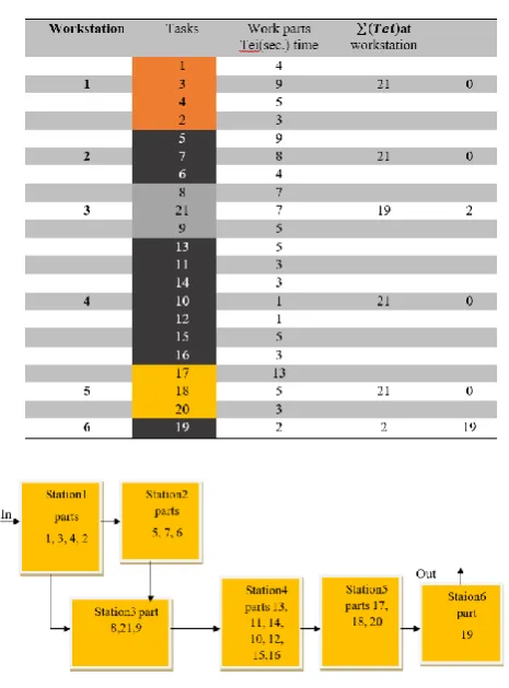
Table 13 Work Parts Assigned to Workstations after Running the Program
Fig. 12 Configuration Layouts for Assembly Line of GA Result
Case1
Assuming that constant demand that means the cycle time (C) for both benchmark problems are constant, by reducing the task processing times by 5% the sensitivity graphs below are drawn based on the result obtained by the three algorithms. If ti is the given processing time of task i then, tinew=ti - FF*(ti).
Benchmark problem 1(n=21tasks)
Table 14 List of Work Parts after 5% off task times (n=21tasks)
Work Parts
Task times Tei (Seconds)
Preceded by
1 3.8 -
2 2.85 1
3 8.55 1
4 4.75 3
5 8.55 4
6 3.8 5
7 7.6 5
Work Parts
Task times Tei (Seconds)
Preceded by
8 6.65 6
9 4.75 8
10 0.95 9
11 2.85 9
12 0.95 9
13 4.75 9
14 2.85 7
15 4.75 10,11,12
16 2.85 15
17 12.35 13,16
18 4.75 13,15
19 1.9 14,18
20 2.85 17
21 6.65 2,4
[image:7.595.48.281.146.461.2] [image:7.595.61.273.581.779.2]3,2,4},{5,21,6},{7,8,9,10,12},{11,13,14,15,16},{17,18,19}, {20}].
Task sequences obtained by RPW: - [{1,
3,4,2},{5,7,6},{8,9,11,10,12,15},{13,16,14,18,14,19},{17,2 1},{20}]
[image:8.595.306.549.58.346.2]Task sequences obtained by GA: - [{1, 2,3,4},{21,5 ,6},{7,8,9,10},{11,12,13,15,16, 18},{14,19,17,20}]
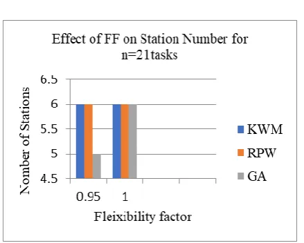
Fig.13 Change in Balance Delay with Change in FF for n=21tasks
Fig. 14 Change in Number of Stations with Change in FF for n=21tasks
Case2
To see the effect of variation of cycle time on the other parameters such as idle time, balance delay and also number of work stations, analysis has done on the two bench mark problems i.e. n=21tasks and n=45tasks.
If C is the given cycle time Cnew=C±constant. Let assume
constant is 2seconds.
Benchmark problem1 (given C=21seconds),
Cnew=19seconds & 23seconds.
Task sequences obtained by KWM at C=19seconds: - [{1,3,2},{4,5,6},{21,7,14},{8,9,10,11,12},{13,15,16,18},{1 7,19,20}]
Task sequences obtained by KWM at C=23seconds: -
[{1,3,2,4},{5,21,6},{7,8,9,10,12},{11,13,14,15,16},{17,18, 19,20}]
Task sequences obtained by RPW at C=19seconds: - [{1,3,4},{5,7
},{6,8,9,11},{10,12,15,13,16,2},{17,18},{20,21,14,19}] Task sequences obtained by RPW at C=23seconds: - [{1,3,4,2},{5,7,6},{8,9,11,10,12,15},{13,16,17},{20,18,21, 14,19}]
Task sequences obtained by GA at C=19seconds: -
[{1,3,2},{4,5,6},{21,7,14},{8,9,10,11,12},{13,15,16,18},{1 7,19,20}]
Task sequences obtained by GA at C=23seconds: -
[image:8.595.50.285.59.388.2][{1, 2, 3, 4},{21, 5, 6},{7, 8, 14, 9},{10, 11, 12, 13, 15,16},{17, 20, 18, 19}]
[image:8.595.60.280.342.518.2]Fig. 15. Change in Balance Delay Time with change Cycle Time for n=21tasks
Table 15 Effect of Change of Cycle Time on Number of Stations Using Three Algorithms for n=21tasks Cycle Time
(Sec.)
Number of Station
KWM RPW GA
19 6 6 6
21 6 6 6
23 5 5 5
I. SUMMARY AND CONCLUSIONS 5.1 Summary
In the present study, the assembly line balancing problem has been solved by heuristic techniques in literature. The heuristic methods such which used in this study are widely used. Even though they are used, they are problem specific. However, GA is a general-purpose line balancing method.
CONCLUSIONS
In this study three heuristic methods /algorithms has been presented to solve simple assembly line balancing problem type-1(SALBP-1). The proposed heuristics were tested by solving the benchmark problem with task number 21 without modifying operation times of the tasks available in literature and by modifying the operation times of the task and Cycle time for the benchmark problem (n=21tasks ). The results compared between the three algorithms based on the objectives achieved, means that the performance measures, namely: - number of workstations, balance delay, balance delay time/total idle time, while the main objective was to minimize the balance delay
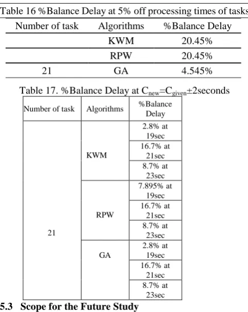
As we observe from table 16 and 17 below there are not differences between the three algorithms used for the sample problems one and two analyzed at the given cycle time in terms of balance delay. But after sensitivity analysis the optimum balance delay obtained. That among the techniques the one which gives the best result is the heuristic treated GA. Table 16 %Balance Delay at 5% off processing times of tasks
Number of task Algorithms %Balance Delay
21
KWM 20.45%
RPW 20.45%
GA 4.545%
Table 17. %Balance Delay at Cnew=Cgiven±2seconds
Number of task Algorithms %Balance Delay
21
KWM
2.8% at 19sec 16.7% at
21sec 8.7% at
23sec
RPW
7.895% at 19sec 16.7% at
21sec 8.7% at
23sec
GA
2.8% at 19sec 16.7% at
21sec 8.7% at
23sec 5.3 Scope for the Future Study
The study in this thesis has done by considering the following two things.
Without modifying (changing) the original data the result analyzed for the benchmark problems selected using the three proposed algorithms.
By modifying the original data for the two benchmark problems that means reducing the processing times by flexibility factor (FF) of 5% and by varying the given cycle time (± constant number on/from the given cycle time ) the result has been analyzed for the two benchmark problems using the three algorithms.
For future work we can incorporate DFMA tools with heuristic methods to achieve the common aim of both methods which is increasing productivity by reducing number of tasks.
REFERENCES
1. Baybars, I. (1986), “A survey of exact algorithms for the simple assembly line balancing problem”. Management Science
2. https://www.pinterest.com/pin/479774166535617906/
3. Bryton, B. (1954), “Balancing of a continuous production line”. Management Sciencethesis. North-Western University.
4. Boysen, N., Fliedner, M., & Scholl, A. (2007), “A classification of assembly line balancing problems”. European Journal of Operational Research.
5. Gutjahr, A. L., &Nemhauser, G. L. (1964), “An algorithm for the line balancing problem”. Management Science.
6. Kim, Y. K., Kim, Y. J., & Kim, Y. (1996), “Genetic algorithms for assembly linebalancing with various objectives”. Computers and Industrial Engineering.
8. Betts, J., & Mahmoud, K. I. (1989), “Identifying multiple solutions for assembly linebalancing having stochastic task times”. Computers & Industrial Engineering,
9. Chica, M., Cordon, O., & Damas, S. (2011), “An advanced multi objective genetic algorithm design for the time and space assembly line balancing problem”. Computers & Industrial Engineering.
10. Manohar, K. R. C., Raghunadh, Y. M., Somanath, B., & Koteswararao,