https://doi.org/10.5194/bg-15-2231-2018 © Author(s) 2018. This work is distributed under the Creative Commons Attribution 4.0 License.
Contribution of fine tree roots to the silicon cycle in a temperate
forest ecosystem developed on three soil types
Marie-Pierre Turpault1, Christophe Calvaruso2, Gil Kirchen1, Paul-Olivier Redon3, and Carine Cochet1
1UR 1138, INRA “Biogéochimie des Ecosystèmes Forestiers”, Centre INRA de Nancy, Champenoux, 54280, France 2EcoSustain, Environmental Engineering Office, Research and Development, Kanfen, 57330, France
3Andra, Direction de la Recherche et Développement, Centre de Meuse/Haute-Marne,
Route départementale 960, Bure, 55290, France
Correspondence:Marie-Pierre Turpault ([email protected]) Received: 2 November 2017 – Discussion started: 27 November 2017
Revised: 18 March 2018 – Accepted: 23 March 2018 – Published: 17 April 2018
Abstract. The role of forest vegetation in the silicon (Si) cycle has been widely examined. However, to date, little is known about the specific role of fine roots. The main objec-tive of our study was to assess the influence of fine roots on the Si cycle in a temperate forest in north-eastern France. Silicon pools and fluxes in vegetal solid and solution phases were quantified within each ecosystem compartment, i.e. in the atmosphere, above-ground and below-ground tree tis-sues, forest floor and different soil layers, on three plots, each with different soil types, i.e. Dystric Cambisol (DC), Eutric Cambisol (EC) and Rendzic Leptosol (RL). In this study, we took advantage of a natural soil gradient, from shallow calcic soil to deep moderately acidic soil, with sim-ilar climates, atmospheric depositions, species compositions and management. Soil solutions were measured monthly for 4 years to study the seasonal dynamics of Si fluxes. A budget of dissolved Si (DSi) was also determined for the forest floor and soil layers. Our study highlighted the major role of fine roots in the Si cycle in forest ecosystems for all soil types. Due to the abundance of fine roots mainly in the superfi-cial soil layers, their high Si concentration (equivalent to that of leaves and 2 orders higher than that of coarse roots) and their rapid turnover rate (approximately 1 year), the mean annual Si fluxes in fine roots in the three plots were 68 and 110 kg ha−1yr−1 for the RL and the DC, respectively. The turnover rates of fine roots and leaves were approximately 71 and 28 % of the total Si taken up by trees each year, demon-strating the importance of biological recycling in the Si cycle in forests. Less than 1 % of the Si taken up by trees each year accumulated in the perennial tissues. This study also
demonstrated the influence of soil type on the concentration of Si in the annual tissues and therefore on the Si fluxes in forests. The concentrations of Si in leaves and fine roots were approximately 1.5–2.0 times higher in the Si-rich DC com-pared to the Si-poor RL. In terms of the DSi budget, DSi production was large in the three plots in the forest floor (9.9 to 12.7 kg ha−1yr−1), as well as in the superficial soil layer (5.3 to 14.5 kg ha−1yr−1), and decreased with soil depth. An immobilization of DSi was even observed at 90 cm depth in plot DC (−1.7 kg ha−1yr−1). The amount of Si leached from the soil profile was relatively low compared to the annual uptake by trees (13 % in plot DC to 29 % in plot RL). The monthly measurements demonstrated that the seasonal dy-namics of the DSi budget were mainly linked to biological activity. Notably, the peak of dissolved Si production in the superficial soil layer occurred during winter and probably re-sulted from fine-root decomposition. Our study reveals that biological processes, particularly those involving fine roots, play a predominant role in the Si cycle in temperate forest ecosystems, while the geochemical processes appear to be limited.
1 Introduction
tem-perate forests (Bartoli, 1983; Watteau and Villemin, 2001; Gérard et al., 2008; Cornelis et al., 2010a, 2011; Sommer et al., 2006, 2013). Several review papers described how dis-solved Si (DSi) in soil is taken up by vascular plants and translocated into biogenic Si (BSi) in an opal form, which is deposited into the cell walls, cell luminas and intercellu-lar spaces (Jones and Handreck, 1965; Conley, 2002; Cor-nelis et al., 2010b; Struyf and Conley, 2012). These struc-tures are called phytoliths. Other important producers of BSi are sponges and protists (diatoms, testate amoebae) (Struyf and Conley, 2012; Sommer et al., 2006; Puppe et al., 2014, 2015). In terrestrial ecosystems BSi pools can be separated into phytogenic (phytoliths), microbial and protozoic pools. The latter is represented in soils by idiosomic testate amoe-bae (Puppe et al., 2014).
According to Conley (2002), the annual fixation of DSi in terrestrial ecosystems has been estimated to range from 60 to 200 Tmoles. That represents 10 to 40 times more than yearly exported DSi and suspended BSi from the terrestrial geobiosphere to the coastal zone (Conley, 2002). Vegetation can thus be considered a product of BSi which returns to the soil as organic matter through biological recycling. Because BSi in general is more soluble than silicate minerals, BSi strongly contributes to the DSi pool (Fraysse et al., 2009; Cornelis and Delvaux, 2016).
Based on the assumption that the storage of Si is limited in roots (Bartoli and Souchier, 1978) and because fine-root sampling and cleaning before analyses are long and tedious processes, studies in forest ecosystems mainly focus on the importance of litterfall recycling in the Si biogeochemical cycle without quantifying Si in the roots (Gérard et al., 2008; Cornelis et al., 2010a; Sommer et al., 2013).
However, Krieger et al. (2017) recently showed that Si in deciduous trees (European beech, Fagus sylvatica and sycamore, Acer pseudoplatanus) generally precipitates as a thin layer (<0.5 µm) around the cells, especially in roots and bark. These small-scale phytogenic Si were demon-strated to influence various soil and plant processes (Meu-nier et al., 2017; Puppe et al., 2017). Maguire et al. (2017), who examined the impact of climate change on Si uptake by trees, observed that fine roots of sugar maple (Acer
sac-charum), which represented only 4 % of the tree’s biomass,
accumulated 29 % of the Si.
Considering the high Si content of fine roots (Krieger et al., 2017; Maguire et al., 2017) and their rapid turnover in forest ecosystems (approximately 1 year in beech forests in Europe; Brunner et al., 2013), we hypothesized that fine roots could significantly contribute to the input of BSi into the soil.
To test this hypothesis, during a 4-year observation period we quantified (i) the total and annual accumulations of Si in stand below-ground and above-ground biomasses while dis-tinguishing annual and perennial compartments, and (ii) the Si input fluxes in the forest floor (litterfall and small woods, above-ground exploitation residues) and in the soil (fine roots
and below-ground exploitation residues). The study took place in a lowland (low lateral transfer of material) decid-uous temperate forest developed on three soils, ranging from a shallow calcic soil to a deep acidic soil, with mull to acid mull humus. These humus forms quickly degrade and con-tain few soil particles and no roots, thus allowing determina-tion of the DSi issued from the degradadetermina-tion of organic layers contrary to mor or moder humus forms (Sommer et al., 2006; Cornelis et al., 2010a). In addition, we quantified the DSi in-puts and outin-puts in these ecosystems monthly, i.e. rainfall, foliar leaching and drainage, in order to assess the seasonal dynamics of these fluxes induced by biological activities.
2 Materials and methods 2.1 Experimental site
The experimental site, hereafter referred to as the Mon-tiers site (http://www.nancy.inra.fr/en/Outils-et-Ressources/ montiers-ecosystem-research, last access: 12 April 2018), is located in the Montiers-sur-Saulx beech forest in north-eastern France (Meuse, France, latitude 48◦3105400N, lon-gitude 5◦1600800E). The site is 73 ha and has been man-aged jointly by the INRA-BEF (French National Institute for Agricultural Research – Biogeochemical cycles in Forest Ecosystems research unit) and by the ANDRA (French Na-tional Radioactive Waste Management Agency) since 2012. The different steps of site establishment are described in de-tail in Calvaruso et al. (2017). The Montiers site is part of different national and international research networks, i.e. SOERE-OPE (Long-lasting observation and experimenta-tion for the research on environment – Perennial Environ-ment Observatory; http://www.andra.fr/ope/index.php?lang= en&Itemid=127, last access: 12 April 2018) and F-ORE-T (Functioning of Forest Ecosystems; http://www.gip-ecofor. org/f-ore-t/, last access: 12 April 2018), and AnaEE (Analy-sis and Experimentations on Ecosystems; https://www.anaee. com/, last access: 12 April 2018). The mean annual rainfall and temperature over the last 20 years were 1069 mm and 9.8◦C, (calculated from Météo-France data). The geology of the Montiers site consists of two overlapping soil parent ma-terials: an underlying Tithonian limestone surmounted by de-trital acidic Valanginian sediments. The calcareous bedrock mainly contains calcium carbonate and∼3.4 % clay miner-als. The overlying detrital sediments are complex, as they re-sult from various depositions and are composed of silt, clay, coarse sand and iron oxide nodules (for more details, see Calvaruso et al., 2017). The site is covered by a homoge-neous stand of the same age (approximately 50 years old in 2010) with the same management approaches. The stand was mainly composed of beech (89 %) and 11 % of other decidu-ous species, i.e. sycamore maple (Acer pseudoplatanus), ash
(Fraxinus excelsior), pedunculate oak (Quercus robur L.),
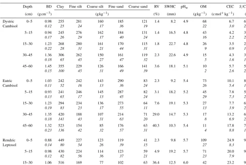
Table 1.Physicochemical properties of the three studied soils at the Montiers site (plot DC, plot EC, plot RL). Presented are the mean values for bulk density (BD), textural distribution (clay, fine silt, coarse silt, fine sand and coarse sand), total rock volume (RV), soil water holding capacity (SWHC), soil water pH (pHw), organic matter content (OM), cation exchange capacity (CEC; cmol+kg−1) and base-cation saturation ratio (S/CEC, withSas the sum of base cations). SD values are given in italics. Table adapted from Kirchen et al. (2017).
Depth BD Clay Fine silt Coarse silt Fine sand Coarse sand RV SWHC pHw OM CEC S/CEC
(cm) (g cm−3) (g kg−1) (%) (mm) (g kg−1) (c mol+kg−1) (%)
Dystric 0–5 0.98 255 281 160 185 121 1.4 8.2 4.9 68 6.7 64.2
Cambisol 0.12 25 24 17 36 19 22 3.0 23.4
5–15 0.94 245 276 162 184 131 1.4 16.5 4.8 43 4.2 35.0
0.17 26 29 17 40 24 16 2.2 20.9
15–30 1.23 268 280 161 170 115 1.8 22.7 4.8 26 3.5 25.9
0.22 28 31 21 44 31 9 0.9 14.1
30–45 1.36 306 262 150 161 119 2.3 22.6 4.9 15 4.3 36.2
0.18 65 45 27 47 32 5 1.6 15.8
45–60 1.45 355 229 126 166 141 3.6 18.1 5.1 10 5.7 55.1
0.15 100 45 31 49 39 2 2.6 21.9
Eutric 0–5 1.03 242 242 143 290 83 2.3 9.2 5.4 73 10.1 83.3
Cambisol 0.11 52 16 13 36 24 26 5.4 14.2
5–15 0.93 241 246 145 287 82 3.1 18.2 5.2 45 7.8 59.1
0.13 65 17 13 45 24 29 7.3 23.6
15–30 1.23 294 234 136 273 64 7.6 19.1 5.3 27 7.7 60.9
0.19 83 23 17 55 11 13 3.9 23.3
30–45 1.35 420 188 107 214 71 29.0 14.7 5.3 17 13.2 68.4
0.18 141 43 31 63 20 8 6.9 27.2
45–60 1.32 523 154 85 176 63 40.3 10.3 5.4 11 17.8 75.6
0.23 136 42 32 57 31 4 8.8 17.4
Rendzic 0–5 0.88 449 227 123 119 41 2.3 9.8 5.7 109 24.9 97.8
Leptosol 0.14 80 54 26 39 15 27 8.3 5.4
5–15 0.98 430 224 114 123 59 4.9 19.2 5.7 71 20.0 94.2
0.12 82 56 36 37 21 23 7.9 6.6
15–30 1.06 516 169 77 102 63 36.4 12.5 6.0 42 23.2 99.3
0.22 81 50 38 42 24 10 6.4 5.3
(Prunus avium). The site is also composed of three different
soil types, i.e. Dystric Cambisol (DC), Eutric Cambisol (EC) and Rendzic Leptosol (RL) (FAO, 2016). A schematic repre-sentation of the soil profiles and their locations are presented in Kirchen et al. (2017). Table 1 presents the main char-acteristics of these different soil types, ranging from acidic and deep soils to calcic and superficial soils, developed on acidic Valanginian and detritic sediments and Portlandian limestone, respectively. Humus type is a eutrophic mull for the RL and EC and an acidic mull for the DC.
Three experimental plots, with an area of 1 ha each, were built on the three different soils to monitor water and element fluxes as well as tree growth over 4 years. Each plot was sub-divided into four subplots (replicates) of which three were equipped with the same monitoring devices designed for the sampling of above-ground and below-ground solutions at dif-ferent depths, soil at difdif-ferent depths, organic horizons and litterfall, and four were equipped with devices for standing above-ground and below-ground biomasses as well as tree growth. In addition, a 45 m high flux tower was placed within
the site (close to plot DC) to collect rainfall and atmospheric deposits.
2.2 Sampling
2.2.1 Solutions and dust deposits
Solutions and dust deposits were sampled every 4 weeks between January 2012 and December 2015, representing 4 years of monitoring.
The throughfall was collected in each replicate by 4 polyethylene gutters (0.39 m2opening), placed 1.2 m above the forest ground.
The stemflow was collected in each replicate on six trees of different sizes using polyethylene collars attached hori-zontally to the stem at 1.50 m. Trees were chosen to cover most of the range of stem circumferences at 130 cm height (C130) in each plot. To prevent the solution from freezing, the stemflow was collected in underground storage contain-ers during the winter.
The gravitational soil solutions (zero-tension lysimeters, ZTL) were collected beneath the forest floor and at different soil depths,−10 and−30 cm (in DC, EC and RL),−60 cm (in DC and EC) and−90 cm (in DC), with large plate lysime-ters (40 cm×30 cm, 0.12 m2; 3 repetitions per soil depth and per replicate) or thin rod-like lysimeters (0.07 m2; in clusters of 8; 3 repetitions per soil depth and per replicate).
The bound soil solutions (tension lysimeters, TL) were collected with ceramic cups inserted into the soil at different depths,−10 and−30 cm (in DC, EC and RL),−60 cm (in DC and EC) and−90 cm (in DC), with four repetitions per depth and per replicate. These ceramic cups were connected to an electric vacuum pump that maintained a constant de-pression between−0.5 and−0.6 bar.
2.2.2 Tree compartments
Three beech trees were harvested in each plot in 2009 to col-lect stem wood, stem bark and branches. Subsequently, the branches were separated into different classes, i.e.<4, 4–7 and >7 cm in diameter, according to Henry et al. (2011). The detailed procedure for collecting stem wood, stem bark and branches is described in Calvaruso et al. (2017).
The fine roots (<2 mm diameter) were collected during March–April 2011 in three soil pits (approximately 0.4 m wide) for each replicate, where the soil material was cut and extracted by layer (0–5, 5–15, 15–30, 30–45, 45–60 and 60–90 cm, when possible). A two-step procedure was applied to accurately assess the fine-root biomass (Bakker et al., 2008), without having to transport the soil to the lab-oratory. The first step involved collecting, in situ, the fine roots from the block of soil extracted from each soil layer. Then, a part of the soil block (approximately 2 kg) was col-lected. The second step, at the laboratory, consisted of using a tweezer to collect all the remaining fine roots in this soil aliquot. This second step allowed for the assessment of the fraction of fine roots uncollected during the first step. The fine roots collected during the two steps were washed at the laboratory, dried in a stream air drier for 3 days and then weighed. For each layer, the total biomass of fine roots was obtained by summing the fine-root biomass collected dur-ing the first step and the fine-root biomass collected durdur-ing the second step and was multiplied by the ratio of total soil block mass/soil aliquot mass. Roots with a diameter>2 cm (small and coarse roots) were collected in February 2017 in
three soil pits (approximately 0.4 m wide) for each plot where soil material was cut and extracted at approximately 20 cm depth. This method does not allow quantification of small-and coarse-root biomass, which were determined through al-lometric equations (Le Goff and Ottorini, 2001). An aliquot of each root sample (fine, small and coarse) was then col-lected to determine element concentration. Each aliquot was carefully washed under a binocular microscope with distilled water, using tweezers and an ultrasound gun. The absence of soil particles was carefully checked on each root sample un-der a binocular microscope with a magnification of 10×. The operation was repeated until all soil particles were removed to prevent soil pollution in the root analyses. A second check using a scanning electron microscope (SEM) equipped with an energy-dispersive X-ray spectrometer (EDX) was carried out on 12 randomly selected subsamples of fine roots by plot (for more details, see Sect. 2.3.4). All observed subsamples were free from soil particles.
The litterfall was collected in six litter traps (0.34 m2each) per replicate. The litter was harvested seven times per year, avoiding litter degradation in the litter traps. During the har-vest, the litter was separated into three compartments, i.e. (i) leaves, (ii) buds, beechnuts and fruit capsules as well as (iii) small branches falling from the trees. The leaves, buds, beechnuts and fruit capsules belong to annual tree compart-ments (recycling each year), while small branches belong to perennial compartments.
2.2.3 Forest floor
We defined the forest floor by the set of organic horizons (Oln, Olv, Of and Oh) above the organo-mineral horizon (Ah) and the small dead wood at the soil surface.
Organic horizons were collected in June 2010 in a cali-brated metal frame (surface area of 0.1 m2). Nine samples were collected in each replicate. Because the lower organic horizons were in direct contact with the superficial soil layer, it was very difficult to sample them without soil contamina-tion. The presence of soil particles, very rich in Si, mixed with the organic horizons, can induce a drastic overestima-tion of the Si pool in this compartment. As a result, we de-cided to carefully sample, on site, six organic horizon sam-ples without the fraction contacting the soil, called “pure or-ganic horizons”. These pure oror-ganic horizons were used to determine the soil fraction in the organic horizon collected on the three plots (see the method in Sect. 2.4.2).
Small dead wood from the previous thinning (winter 2009–2010) was harvested in June 2010 at the three plots in a calibrated metal frame (surface area of 0.6084 m2). Nine samples were collected in each replicate, according to a grid. 2.2.4 Soil
extracted through an auger by layers 0–5, 5–15, 15–30, 30– 45, 45–60 and 60–90 cm, when possible.
2.3 Analytical methods 2.3.1 Si content in solutions
Solutions of rainwater, stemflow, throughfall, forest floor and soil were filtered at 0.45 µm, stored at 4◦C and analysed
during the week following the sampling. The Si content in the solutions was measured by inductively coupled plasma-atomic emission spectrometry (ICP-AES Agilent Technolo-gies 700 type ICP-OES, Santa Clara, USA).
2.3.2 Si content in biomass
Samples from the above-ground and below-ground compart-ments of the trees, litterfall and forest floor were dried in a stream air-drier (at 65◦C), then ground and encapsulated for analysis. The total Si content in the biomass was assessed by X fluorescence using an X fluorescence sequential spec-trometer S8 TIGER 1 kW (Bruker, Marne la vallée, France). 2.3.3 Si content in soil and dust deposits
The total Si content in soil organo-mineral and mineral layers (preliminarily sieved at 2 mm) and in dust deposits was deter-mined by inductively coupled plasma-atomic emission spec-trometry (700 Series ICP-OES, AGILENT TECHNOLO-GIES) after alkaline fusion in LiBO2and in HNO3.
2.3.4 Microscopic analysis
Between 9 and 12 randomly selected samples of fine roots, stem and branch bark, fruit capsules, bud scales and fresh and altered leaves (from organic horizons) collected on beech trees for each plot were mounted on glass plates using double-coated carbon conductive tabs and covered with carbon. These samples were examined at the GeoRes-sources laboratory (University of Lorraine) for biomineral occurrence and composition using a Hitachi S-4800 SEM equipped with an EDX and containing a lithium-drifted Si detector. The SEM analyses were carried out using an accel-eration voltage of 10 or 15 kV.
2.4 Calculation of Si pools and fluxes in solutions and solids
In each plot, Si fluxes and pools were obtained by multiply-ing the amount of solution or solid by the concentration of Si in the given compartment. All monthly Si fluxes were calcu-lated on a 1 ha basis and were summed over calendar years to compute the annual fluxes. The DSi budget was also cal-culated for forest floor and soil layers using the difference between input and output fluxes.
In the following sections (2.4.1 to 2.4.10), we will only present the Si fluxes or pools for which the method of
calcu-lation differs from that of the calcucalcu-lation of multiplying the amount of solution or solid by the concentration of Si in the compartment.
2.4.1 Dust deposits
To take into account the loss of particles during the collection of dust deposits from rainfall, a test using standard minerals was done to assess the efficiency of the procedure (Lequy et al., 2014). The efficiency was estimated at 72 %. Thus, the total weight of dust deposits per year was determined as the weight of dust deposits collected on site, divided by a correc-tion factor of 0.72.
2.4.2 Organic horizons
The percentage of soil mixed with the organic horizons was determined through the use of titanium (Ti). This element is a good tracer of soil pollution in the collected organic horizons because Ti is in very low abundance in pure or-ganic horizons (<0.3 mg kg−1), but more abundant in soils (>4 mg kg−1). We measured Ti content in the soil surface layer (0–5 cm), in the pure organic horizons and in the or-ganic horizons collected on the three plots. The percentage of soil in the organic horizons was calculated using Eq. (1): Soil %= [(TiHb−TiHp)/(TiS−TiHp)], (1)
where TiHbis the concentration of Ti in the organic horizons,
TiHpis the concentration of Ti in the pure organic horizons,
and TiSis the mean concentration of Ti in the 0–5 cm horizon
of soil for each plot. The mean soil fraction represented less than 5% of the total organic horizon mass in our study. The fraction of Si introduced by soil contamination was deducted to obtain the Si content in the organic horizons.
2.4.3 Stemflow and stand deposition
To transform the stemflow volumes into a water flux, C130 was assumed to explain the stemflow volume variability be-tween individuals within a species. Thus, all the trees in each plot were separated into several C130 classes, and the corre-lation between the stemflow volume and the C130 was veri-fied for the entire sampling period. Using a trend line equa-tion, a mean monthly stemflow volume was then assigned to each C130 class. The stemflow at the plot scale for a given C130 class (SFz; in mm) is given by following Eq. (2):
SFz=Vz·
Nz
A
, (2)
wherezis the C130 class,Vzis the mean stemflow volume
per tree in the given C130 class (in L),Nzis the number of
The Si stand deposition, i.e. the amount of Si (kg ha−1yr−1) reaching the soil after crossing over the
canopy, was determined as the sum of the Si fluxes in throughfall and stemflow.
2.4.4 Drainage flux
The BILJOU©model (Granier et al., 1999) was applied in the three plots at the Montiers site to assess the water drainage flux for the different soil layers. The detailed procedure and the data are presented in Kirchen et al. (2017). The gravi-tational water flux was determined for each soil layer and date from the collected gravitational volume. The bound wa-ter flux was obtained by subtracting the wawa-ter gravitational flux from the modelled water drainage flux. In this study, we determined that the water gravitational flux/water bound flux ratio was approximately 80/20, which is similar to the measurement from a Cl tracer in a beech temperate forest in Fougères (western France) in Legout et al. (2009).
Thus, the monthly drainage fluxes of the elements were calculated at each depth following Eq. (3):
DSi=DG·CSiG+DB·CSiB, (3)
whereDSiis the drainage flux of Si,DGis the water drainage
via rapid gravitational transfer, CSiG is the concentration
of Si in the gravitational soil solution collected with zero-tension lysimeters,DBis the water drainage via slow bound
transfer, andCSiBis the concentration of Si in the bound soil
solution collected in ceramic cups.
The element mass balances were calculated for the fol-lowing soil layers, according to the installation depths of the lysimeters in the three plots: forest floor, from the forest floor to −10 cm, between −10 and −30 cm, between −30 and
−60 cm and between−60 and−90 cm. For each soil layer, the mass balance of the elements was calculated as the dif-ference between the drainage at the bottom of the layer and the drainage entering the layer (Eq. 4):
MBSi=DSi2−DSi1, (4)
where MBSi is the mass balance of Si in a given soil layer,
DSi1 is the incoming drainage flux of Si, andDSi2 is the
drainage flux at the bottom of the soil layer. 2.4.5 Above-ground tree biomass
The evaluation of above-ground tree biomass was calcu-lated according to procedures described in Saint-André et al. (2005). It included four steps: (i) the circumference of all trees was measured at 130 cm height, C130, in autumn
2011 and 2015; (ii) eight trees in each plot, representing the range of C130, stem bark and wood and 0–4, 4–7 and
>7 cm diameter branches were sampled; (iii) the weighed allometric equations fitted for each ecosystem compartment were calculated according to Calvaruso et al. (2017); and
(iv) tree biomass (stem bark and wood and 0–4, 4–7 and >7 cm diameter branches) was quantified per hectare by applying fitted equations to the stand inventories. Annual above-ground biomass production and Si immobilization in above-ground biomass were calculated as the difference be-tween the biomass or Si amount in the biomass calculated for 2015 and 2011, divided by four.
2.4.6 Fine-root flux
The fine-root turnover rate is dependent on the fine-root biomass and the annual production but also on the various methods and calculations used to determine the rate (Jour-dan et al., 2008; Gaul et al., 2009; Finer et al., 2011; Yuan and Chen, 2010). In this study, the annual fine-root produc-tion was calculated by using the mean fine-root turnover rate of 1.11±0.21 y−1, issued from the last available European
data compilation for beech forests (Brunner et al., 2013). The turnover rate corresponds to the ratio between the produc-tion of fine roots during the growing season and the mean biomass of living fine roots during the year. The Si flux from fine roots was calculated by multiplying the annual fine-root production by the Si concentration in the fine roots.
2.4.7 Small and coarse roots
The small- and coarse-root biomass as well as the annual root increment were determined using allometric equations, linking the stem diameter at breast level and root biomass of beech trees (Le Goff and Ottorini, 2001).
The pools and fluxes of Si in small and coarse roots were calculated by multiplying the total biomass or the annual root increment by the Si concentration in small and coarse roots. 2.4.8 Exploitation residuals and harvest
To take into account the influence of forestry practices after 2010 on the Si cycle, we simulated a stand thinning based on the forestry practices applied in the Montiers massif by the French National Forestry Office. At this stage of stand devel-opment, the National Forestry Office carries out a thinning every 7 years, with an above-ground biomass cut of approx-imately 40×103kg ha−1. Because the amount of biomass cut is dependent on the stand above-ground biomass, we in-tegrated this parameter into our calculation of exploitation residuals and harvest.
We determined that the above-ground biomass that will be cut during the next thinning (winter 2017–2018) will be ap-proximately 40.0, 44.3 and 35.0×10³kg ha−1in plots DC, EC and RL. The root biomass remaining from this thinning will represent approximately 7.9, 9.6 and 6.9×10³kg ha−1 in plots DC, EC and RL.
of residuals (<4 and 4–7 cm diameter branches) and exports (>7 cm diameter branches, stem wood and bark) issued from this thinning for each plot. The roots were not exported.
Because thinning in this region is generally done every 7 years, we obtained the annual Si amounts returned to the soil and exported by dividing the total exploitation residuals by seven.
2.4.9 Foliar leaching
The amount of Si released in foliar leachates throughout the year (SiFL, in kg Si ha−1yr−1) was calculated using Eq. (5):
SiFL=SiSD−SiR, (5)
where SiSD is the amount of Si in the stand
deposi-tion throughout the year, and SiR is the amount of Si
in annual rainfall. All these parameters were assessed in kg Si ha−1yr−1.
2.4.10 Tree uptake
The amount of Si taken up by trees throughout the year (SiUp,
in kg Si ha−1yr−1) was calculated using Eq. (6):
SiUp=SiIAG+SiIBG+SiRFL, (6)
where SiIAG is the amount of Si immobilized in the
to-tal above-ground biomass of trees (stem bark and wood, branches, leaves and buds, beechnuts and fruit capsules) throughout the year, SiIBGis the amount of Si immobilized
in the total below-ground biomass of trees (coarse, small and fine roots) throughout the year, and SiRFLis the amount of
Si released in foliar leachates throughout the year. All these parameters were assessed in kg Si ha−1yr−1.
2.5 Statistical analysis
The descriptive statistical parameters (e.g. mean, SD, varia-tion coefficient) were performed using XLSTAT 2017 soft-ware. The normality of the distribution was checked using the Shapiro–Wilk test. As our data did not follow a nor-mal distribution, the non-parametrical Kruskal–Wallis test was performed to determine the significance of differences in biomass pools and increments, Si content, pools and fluxes for each tree compartment, total Si content and pool in soil, and Si content and fluxes in soil solutions between the three soils, at the threshold level of 0.05. The post hoc Bonferroni correction was used for the pairwise comparison. The non-parametrical Mann–Whitney U test was also performed to determine the significance of differences in Si content and Si fluxes between gravitational and bound solutions by soil layer for each soil type, at the threshold level of 0.05.
3 Results 3.1 Si in solids
3.1.1 Microscopic observations of Si deposits in vegetation and the forest floor
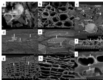
In fresh leaves, Si precipitates in cell walls but also in in-tercellular spaces, generally forming Si deposits called phy-toliths, which are several micrometres (Fig. 1a). In all tree compartments except wood, these Si deposits mostly oc-curred as fine coating layers thinner than 0.3 µm in the in-ner cell walls of fruit capsules (Fig. 1b), stem bark (Fig. 1d and e), bud scales (Fig. 1f) and roots (Fig. 1g–i). The cells covered with Si deposits were in the external parts of the roots, branches and stem bark (Fig. 1d and g). Occasionally, Si was present on cell lumina (Fig. 1e).
Aged leaves in the organic horizon were colonized by hy-phae and amoebae (Fig. 1c) and presented large voids. The Si deposits disappeared from the plant cells but were present in the observed testate amoebae.
3.1.2 Si pools and fluxes in above-ground tree biomass The calculated standing above-ground biomass in 2011 in-creased as RL<DC<EC, with significant differences be-tween EC and RL (factor of 1.4) (Table 2). The stem bark had the highest Si concentration in the three plots, and the Si pool in this compartment represented approximately 40 % of the total Si pool in the above-ground tree biomass. The younger the structures were, the higher the Si concentration. Small branches were approximately 3 times more concentrated than coarse branches in the three soils (Table 2). The amount of Si immobilized in the standing above-ground biomass ranged from 20.1 kg ha−1on the RL to 26.2 kg ha−1on the EC. The annual biomass production between 2011 and 2015 increased as RL<EC<DC, with significant differences between DC and RL (factor of 1.7). As a result, the amount of Si immobi-lized in the above-ground biomass each year between 2011 and 2015 ranged from 0.98 kg ha−1on the RL to 1.82 kg ha−1 on the DC.
Figure 1.Si in biological tissues of beech trees observed with scanning electron microscopy.(a)Si precipitates in the intercellular space of fresh leaves, forming phytoliths (vertical white arrow). Deposits of Si (white arrows) in the inner cell walls of fruit capsules(b), stem bark (dande), bud scales(f)and roots (g,handi).(c)Hyphae, testate amoebae and large voids in aged litter leaves. Si deposits are only present in the testate amoeba shells (horizontal empty white arrows). The presence of Si was confirmed with EDX (analysed zones indicated by white vertical arrows).
1.11±0.21 y−1, we calculated that the annual Si fluxes re-sulting from fine-root decomposition overpassed 100 kg ha−1 in the DC.
The calculated small- and coarse-root biomass was 3 times higher than that of the fine roots, thus representing approx-imately 75 % of the total root biomass in the three plots, but the concentrations of Si in coarse roots were 2 orders of magnitude lower than the concentration in fine roots. As observed for fine roots, the Si concentrations in coarse roots were higher in the DC compared to the RL. The annual im-mobilization of Si in coarse roots was very low for the three soils and was negligible in comparison to the flux induced by fine-root functioning.
3.1.4 Si fluxes in exploitation residues and harvests
The biomass of below-ground and above-ground ex-ploitation residues expressed on an annual basis over-passed 2.0×10³kg ha−1yr−1 (Table 2), with a 1:1 ratio below-ground/above-ground. The above-ground exploita-tion residues were 3 to 6 times more concentrated in Si than the below-ground ones. The amount of Si returning to the soil through exploitation residues was lower than 0.50 kg ha−1yr−1. This value was very close to the amount
of Si exported from the ecosystem through harvests induced by dynamic forestry practice on the study site.
3.1.5 Si pool in forest floor
In 2010, the forest floor biomass drastically differed between the different soil types, about 2 times more on the DC (acid mull) compared to the RL (eutrophic mull). Part of the small wood (residuals from the previous thinning) was higher in the DC compared to the other two soil types, which made up approximately 40 and 20 % of the total forest floor (Ta-ble 2). The Si pools in the forest floor ranged from about 150 kg ha−1on the RL to about 250 kg ha−1on the DC. Be-cause organic horizons have higher concentrations of Si than small woods, organic horizons represented more than 95 % of the Si pools in the forest floor.
3.1.6 Si fluxes in litterfall
Table 2.Mean Si contents, pools and fluxes in the biomass of the three soils at the Montiers site. SD values are given in brackets. Values with different letters are significantly different according to a Kruskal–Wallis test at the thresholdP value level of 0.05 (soil effect; DC, EC and RL). B+W stands for bark and wood.
Plot Compartment Biomass pools
(t DM ha−1) Biomass increment(t DM ha−1yr−1) Si content(g kg−1) Si pools(kg ha−1) Si fluxes(kg ha−1yr−1)
Dystric Cambisol Leaves 3.8 (0.4)a 3.8 (0.4)a 11.3 (1.8)b 42.7 (4.3)b 42.7 (4.3)b Branches/twigs with bark 0.3 (0.2)a 0.3 (0.2)a 1.1 (0.3)a 0.3 (0.2)a 0.3 (0.2)a Buds, beechnuts, fruit capsules 1.1 (1.1)a 1.1 (1.1)a 2.4 (1.0)a 1.8 (0.9)a 1.8 (0.9)a
Total litterfall 5.2 (1.1)a 5.2 (1.1)a 44.8 (5.1)b 44.8 (5.1)b
Organic horizons 11.5 (2.0)a 21.4 (1.6)a 246.4 (53.1)a Small wood 7.5 (1.9)a 0.8 (0.3)a 6.5 (3.5)a Forest floor 19.0 (2.7)a 252.9 (53.1)a
Stem bark 5.5 (0.7)a 0.5 (0.0)b 1.70 (0.33)a 9.4 (1.2)a 0.65 (0.03)b Stem wood 84.8 (11.7)ab 6.4 (0.3)b 0.05 (0.00)a 4.0 (0.5)a 0.30 (0.02)a Small branches (B+W) 18.7 (2.5)ab 1.2 (0.1)b 0.40 (0.05)a 7.4 (1.0)a 0.49 (0.03)b Medium branches (B+W) 10.2 (1.8)ab 1.1 (0.1)b 0.26 (0.04)a 2.6 (0.5)ab 0.29 (0.02)b Coarse branches (B+W) 5.1 (1.1)ab 0.8 (0.1)ab 0.13 (0.04)a 0.7 (0.1)ab 0.10 (0.01)b Above-ground biomass 125.8 (17.9)ab 10.0 (0.5)b 24.1 (3.3)ab 1.82 (0.10)b
Fine roots (0–10 cm) 3.2 (0.8)a 3.5 (0.9)a 12.8 (2.3)b 39.5 (7.5)a 43.9 (8.3)a
Fine roots (10–30 cm) 2.9 (1.1)a 3.2 (1.2)a 15.0 (2.3)c 43.9 (6.6)b 48.8 (7.3)b Fine roots (30–60 cm) 0.9 (0.6)a 1.0 (0.7)a 12.3 10.5 11.7 Fine roots (60–90 cm) 0.4 (0.1)a 0.4 (0.1)a 12.7 4.7 5.2
Total fine roots (0–90 cm) 7.3 (1.8)a 8.0 (2.0) 98.7 (13.5)b 109.5 (15.0)b
Total coarse roots 24.4 (3.5)a 2.83 (0.47)a 0.11 (0.15)a 2.66 (0.39)b 0.31 (0.05)b
Exploitation residues AG 1.3 0.33 0.42
Exploitation residues BG 1.1 0.11 (0.15)a 0.12
Total exploitation residues 2.4 0.54
Harvests 4.4 0.16 0.71
Eutric Cambisol Leaves 4.1 (0.5)a 4.1 (0.5)a 8.9 (1.6)ab 35.4 (2.8)ab 35.4 (2.8)ab Branches/twigs with bark 0.6 (0.4)a 0.6 (0.4)a 0.9 (0.2)a 0.4 (0.2)a 0.4 (0.2)a Buds, beechnuts, fruit capsules 1.3 (1.1)a 1.3 (1.1)a 3.4 (1.9)a 3.0 (0.5)b 3.0 (0.5)b
Total litterfall 6.0 (1.1)a 6.0 (1.1)a 38.7 (3.1)ab 38.7 (3.1)ab
Organic horizons 9.6 (1.4)a 17.6 (0.8)a 174.2 (32.8)ab Small wood 2.6 (1.2)a 1.8 (1.1)a 3.9 (1.3)a
Forest floor 12.5 (0.6)a 178.1 (32.6)ab
Stem bark 6.1 (0.2)a 0.4 (0.0)ab 1.53 (0.28)a 9.3 (0.3)a 0.39 (0.04)a Stem wood 109.9 (3.8)b 5.0 (0.6)ab 0.05 (0.00)a 5.1 (0.2)a 0.23 (0.02)a Small branches (B+W) 20.8 (0.7)b 0.8 (0.1)ab 0.38 (0.08)a 7.9 (0.3)a 0.31 (0.04)ab Medium branches (B+W) 15.2 (0.6)b 1.0 (0.1)ab 0.23 (0.05)a 3.5 (0.1)b 0.23 (0.02)ab Coarse branches (B+W) 9.8 (0.6)b 0.9 (0.1)b 0.10 (0.03)a 1.0 (0.1)b 0.09 (0.01)ab Above-ground biomass 164.2 (5.7)b 8.0 (0.9)ab 26.9 (0.9)b 1.25 (0.13)ab
Fine roots (0–10 cm) 4.6 (2.1)a 5.1 (2.4)a 9.6 (2.9)ab 44.5 (13.9)a 49.4 (15.4)a Fine roots (10–30 cm) 4.5 (1.8)a 5.0 (1.9)a 8.2 (1.6)b 37.0 (7.1)b 41.1 (7.8)b Fine roots (30–60 cm) 1.2 (0.7)a 1.3 (0.8)a 7.5 8.7 9.7 Fine roots (60–90 cm) 0.4 (0.1)a 0.5 (0.1)a – – –
Total fine roots (0–90 cm) 10.6 (4.1)a 11.7 (4.5) 90.2 (20.8)b 100.1 (23.1)b
Total coarse roots 32.3 (1.2)b 4.08 (0.16)b 0.05 (0.08)a 1.51 (0.05)a 0.19 (0.01)a
Exploitation residues AG 1.4 0.31 0.43
Exploitation residues BG 1.4 0.05 (0.08)a 0.06
Total exploitation residues 2.8 0.50
Harvests 4.9 0.15 0.72
: Rendzic Leptosol Leaves 4.0 (0.4)a 4.0 (0.4)a 5.6 (1.3)a 22.2 (3.1)a 22.2 (3.1)a Branches/twigs with bark 0.5 (0.3)a 0.5 (0.3)a 0.7 (0.1)a 0.3 (0.2)a 0.3 (0.2)a Buds, beechnuts, fruit capsules 1.2 (0.9)a 1.2 (0.9)a 3.2 (1.6)a 2.6 (0.5)ab 2.6 (0.5)ab
Total litterfall 5.7 (1.0)a 5.7 (1.0)a 25.2 (3.4)a 25.2 (3.4)a
Organic horizons 8.8 (1.5)a 16.9 (1.4)a 151.3 (22.6)b Small wood 1.9 (2.4)a 1.3 (0.7)a 4.4 (5.7)a
Forest floor 10.9 (2.8)a 154.3 (25.3)a
Stem bark 6.8 (0.6)a 0.3 (0.0)a 1.34 (0.27)a 9.1 (0.8)a 0.41 (0.05)ab Stem wood 80.1 (8.3)a 3.9 (0.5)a 0.06 (0.03)a 5.0 (0.5)a 0.24 (0.03)a Small branches (B+W) 15.0 (1.4)a 0.6 (0.1)a 0.29 (0.04)a 4.3 (0.4)a 0.18 (0.02)a Medium branches (B+W) 8.6 (1.4)a 0.6 (0.1)a 0.19 (0.04)a 1.6 (0.3)a 0.11 (0.02)a Coarse branches (B+W) 4.6 (1.0)a 0.4 (0.1)a 0.10 (0.03)a 0.5 (0.1)a 0.04 (0.01)a Above-ground biomass 115.2 (12.8)a 5.8 (0.8)a 20.5 (2.1)a 0.98 (0.13)a
Fine roots (0–10 cm) 5.1 (1.4)a 5.6 (1.6)a 7.8 (2.2)a 43.5 (14.1)a 48.3 (15.6)a Fine roots (10–30 cm) 3.6 (1.6)a 4.0 (1.8)a 4.9 (0.8)a 17.6 (3.0)a 19.6 (3.3)a
Fine roots (30–60 cm) NS NS – – –
Fine roots (60–90 cm) NS NS – – –
Total fine roots (0–30 cm) 8.7 (3.0)a 9.6 (3.3) 61.2 (16.0)a 67.9 (17.7)a
Total coarse roots 26.0 (3.0)a 3.09 (0.44)a 0.06 (0.05)a 1.62 (0.19)a 0.19 (0.03)a
Exploitation residues AG 1.1 0.24 0.27
Exploitation residues BG 1.0 0.06 (0.05)a 0.06
Total exploitation residues 2.1 0.33
was higher than the other litterfall compartments, measuring 9–10 times higher than branches/twigs and 2–5 times higher than buds, beechnuts and fruit capsules. Because of their high biomass and Si concentration compared to the other litter-fall compartments, leaves were the main fraction of the Si pool (>90 %) in the litterfall in the three plots. Litter leaves collected in DC were twice as concentrated in Si than litter leaves collected in RL (11.3 against 5.6 g kg−1), meaning that the annual Si flux from litterfall was significantly higher on the DC (44.8 kg ha−1) compared to the RL (25.2 kg ha−1). 3.1.7 Si pool in soils and flux of dust deposits
The total Si content and pools in the fine earth fraction were significantly lower in the RL compared to the DC and to the EC (Table 3). The total Si pools in the first 90 cm of soil overpassed 2.4×10⁶kg ha−1in the DC and EC as opposed to approximately 7.2×10⁵kg ha−1in the RL.
The dust deposit annual flux between 2012 and 2015, col-lected on the flux tower of the DC plot above the canopy represented an annual Si input of approximately 6.0 kg ha−1 (Table 4).
3.2 Si in solution: DSi
3.2.1 Si flux in above-ground solutions
The mean annual Si concentration in the rainfall was very low (Table 4) compared to stand deposition (Table 4), rep-resenting an annual Si flux of approximately 0.2 kg ha−1. Consequently, the stand deposition and foliar leaching did not significantly differ between the three plots (Table 4). In the three plots, the throughfall solution was enriched in Si (Table 4), and its maximum concentration occurred during the leafed period, especially during the senescence period (Fig. 2). Although the stemflow solution was more concen-trated in DSi (Table 4) than the throughfall (Table 4), the throughfall contributed a large amount (up to 85 %) to the Si stand deposition.
3.2.2 Si fluxes in the forest floor
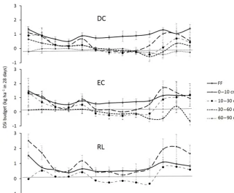
Over the study period (2012–2015), the solution collected under the forest floor was enriched in Si compared to the above-ground one (approximately 1 order of magnitude; Ta-ble 4) and was equivalent in the three soil types. The net Si production in the forest floor was highest between September and January and was at a minimum in April, particularly in plot RL (Fig. 3). The mean annual DSi production in the for-est floor ranged between 12.4 and 9.5 kg ha−1yr−1in plots DC and RL (Table 4).
3.2.3 Si fluxes in the soil profile
Regardless of the soil type, the mean annual DSi concentra-tion generally increased with soil depth for both kinds of
so-lutions, except in the deeper soil layers where the Si concen-tration remained constant (Fig. 4a). The DSi concenconcen-trations in the gravitational solution (ZTL) in the 0 to 30 cm soil lay-ers and in the bound-solutions (TL) in the 0–60 cm soil laylay-ers increased less than in the forest floor. Regardless of the soil type and depth, the TL solutions were more concentrated in DSi than the ZTL solutions (approximately 1.1 to 1.8 times more; Fig. 4a). No matter the depth and the soil type, DSi concentrations in TL solutions showed seasonal variations, with high concentrations between August and December and low concentrations between February and June, which was not the case for ZTL concentrations (Fig. 4b). The maximum concentration of DSi did not depend on the drainage fluxes (data not shown).
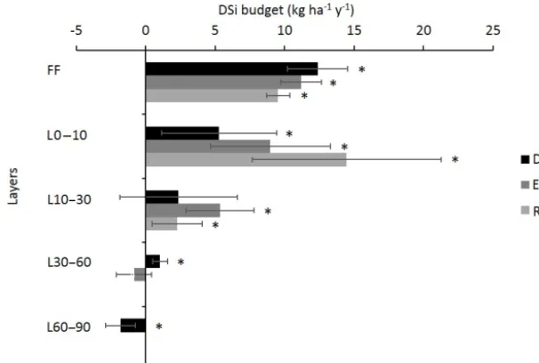
The Si budget revealed a net annual production of DSi in the 0–10 and 10–30 cm layers, respectively ranging from 5.3 kg ha−1yr−1in plot DC to 14.5 kg ha−1yr−1in plot RL
and from 2.3 kg ha−1yr−1 in plot DC to 5.4 kg ha−1yr−1in
plot EC (Fig. 5). The production of DSi drastically decreased with the depth. In the 60–90 cm layer of plot DC, we even observed a decrease in the amount of DSi (Fig. 5), resulting from its immobilization during the autumn (Fig. 3). In addi-tion, we observed high seasonal variations in the DSi budget, which were more marked in the topsoil layers (Fig. 3). The lowest net production in these horizons was between June and August, while the maximum production rates were ob-served between September and February.
3.3 Si flux taken up by trees
By adding the amounts of the Si accumulated each year in the different tree compartments, i.e. perennial above-ground biomass, leaves, bud scales, beechnuts and fruit capsules, small and coarse roots, and fine roots and the foliar leachate, we determined that the annual uptake of Si by the stand was approximately 157, 141 and 95 kg ha−1in plots DC, EC and RL (Fig. 6).
4 Discussion
4.1 Si accumulation and internal fluxes in trees
con-Table 3.Mean total Si content and pool in the fine earth fraction of the three soils at the Montiers site at different depths. SD values are given in brackets. Values with different letters are significantly different according to a Kruskal–Wallis test at the thresholdP value level of 0.05 (soil effect; DC, EC and RL).
Soil type Compartment Total Si content
(g kg−1)
Total Si pool (103kg ha−1)
Dystric Cambisol 0–10 cm 305 (13)a 297 (33)b
10–30 cm 313 (9)a 708 (50)b
30–60 cm 296 (18)b 1 301 (422)b
60–90 cm 230 (28)b 858 (80)c
Total 0–90 cm 3 164 (487)b
Eutric Cambisol 0–10 cm 361 (11)b 411 (30)c
10–30 cm 360 (13)b 791 (127)b
30–60 cm 295 (62)b 871 (290)b
60–90 cm 224 (28)b 348 (117)b
Total 0–90 cm 2 421 (410)b
Rendzic Leptosol 0–10 cm 287 (27)a 233 (18)a
10–30 cm 276 (23)a 427 (27)a
30–60 cm 175 (37)a 42 (27)a
60–90 cm 144 (39)a 27 (8)a
[image:11.612.157.438.108.342.2]Total 0–90 cm 720 (38)a
Table 4.Si content and fluxes in the ZTL (zero-tension lysimeter) and TL (tension lysimeter) solutions of the three soils at the Montiers site. SD values are given in brackets. Values with different letters are significantly different according to a Kruskal–Wallis test at the threshold P value level of 0.05 (soil effect; DC, EC and RL).
Plot Level SiZTLconcentration
(mg L−1)
SiTLconcentration
(mg L−1)
Si fluxes (kg ha−1yr−1)
Dystric Cambisol Rainfall 0.04 (0.08) 0.2 (0.1)
Throughfall 0.15 (0.18)a 1.2 (0.6)a
Stemflow 0.38 (0.32)a 0.1 (0.5)a
Stand deposition 1.3 (0.3)a
Forest floor 1.7 (0.8)a 13.7 (2.7)a
L-10 cm 2.0 (0.7)a 2.9 (1.0)a 19.0 (5.6)a
L-30 cm 2.6 (0.4)a 3.5 (1.1)a 21.4 (8.3)a
L-60 cm 2.6 (0.5)a 4.1 (1.4)a 22.4 (9.8)a
L-90 cm 2.5 (0.3) 3.7 (0.6) 20.7 (7.4)
Eutric Cambisol Rainfall 0.04 (0.08) 0.2 (0.1)
Throughfall 0.16 (0.16)a 1.2 (0.6)a
Stemflow 0.53 (0.38)a 0.2 (0.6)a
Stand deposition 1.4 (0.6)a
Forest floor 1.5 (0.6)a 12.6 (4.2)a
L-10 cm 2.1 (0.7)a 3.2 (1.1)a 21.6 (4.8)a
L-30 cm 3.5 (1.6)a 4.0 (1.1)a 25.5 (5.9)a
L-60 cm 2.8 (0.6)a 4.5 (1.1)a 26.2 (6.6)a
Rendzic Leptosol Rainfall 0.04 (0.08) 0.2 (0.1)
Throughfall 0.13 (0.14)a 1.0 (0.5)a
Stemflow 0.42 (0.41)a 0.1 (0.4)a
Stand deposition 1.2 (0.5)a
Forest floor 1.4 (0.8)a 10.7 (1.4)a
L-10 cm 2.1 (1.1)a 3.8 (1.2)a 25.2 (9.9)a
[image:11.612.104.490.398.707.2]Figure 2.Seasonal dynamics over 4 years (January 2012 to December 2015) of DSi concentration in throughfall solution for the three plots, DC, EC and RL.
Figure 3.Seasonal dynamics over 4 years (January 2012 to December 2015) of the DSi budget in the different layers (forest floor, FF; soil 0–10 cm; soil 10–30 cm; soil 30–60 cm; and soil 60–90 cm) for the three plots, DC, EC and RL.
centration in this compartment (4.9 to 15.0 g kg−1) but also from a large biomass. The Si content in fine beech roots was higher (2 to 6 times) than that measured by Maguire
et al. (2017) for another deciduous species, i.e. sugar maple
(Acer saccharum), but in a cooler environment. Besides
[image:12.612.132.470.346.626.2]in-Figure 4. (a)Mean DSi concentration over 4 years (January 2012 to December 2015) in zero-tension lysimeters (ZTL) and tension lysimeters (TL) at different soil depths (0–10, 10–30, 30–60 and 60–90 cm) in plots DC and RL. For each soil type and depth, values with an asterisk are significantly different according to a Mann– Whitney U test at the thresholdP value level of 0.05 (solution-type effect, ZTL vs. TL).(b)Seasonal dynamics over 4 years (Jan-uary 2012 to December 2015) of DSi concentrations in ZTL and TL in the 0–10 cm and 10–30 cm soil layers of plot RL.
creased soil freezing significantly lowers the Si content of sugar maple fine roots. The fine beech root biomass ranged from 7.3 to 10.6 t ha−1at the Montiers site. These values cor-respond to the upper part of the range of 2.4 to 9.6 t ha−1 reported in the literature for beech stands in Europe (Hen-driks and Bianchi, 1995; Le Goff and Ottorini, 2001; Schmid, 2002; Claus and George, 2005; Bolte and Villanueva, 2006) and are in agreement with the fine-root biomass determined for another beech forest located in north-eastern France (7.4 to 9.8 t ha−1; Bakker et al., 2008).
Because most of the Si accumulated in leaves and fine roots with rapid turnover (annual for leaves and estimated at 1.11±0.21 y−1for fine beech roots; Brunner et al., 2013),
a large part of the Si taken up by trees returned to the soil each year via litterfall degradation (28 %, from 25.2 kg ha−1 in plot RL to 44.9 kg ha−1 in plot DC) and via the de-composition of fine-root necromass (approximately 71 %, from 67.9 kg ha−1 in plot RL to 109.5 kg ha−1in plot DC) (Fig. 6, Table 2). As demonstrated by Sommer et al., 2013, only a small fraction (approximately 1 % in our study; from 1.0 kg ha−1 in plot RL to 1.8 kg ha−1 in plot DC) of the
Si is taken up by the tree stand accumulated each year in the perennial tree compartments, i.e. the stem, branch and coarse roots (Fig. 6, Table 2). As a consequence, approxi-mately 99 % of the Si taken up by the stand each year re-turned to the soil via recycling of fine roots and leaves. The Si that accumulated in the tree stand and returned to the soil (without considering the exploitation residuals) at the Montiers site ranged from 93 to 154 kg ha−1yr−1. This is higher than in other beech ecosystems previously studied, i.e. 20 kg ha−1yr−1(Cornelis et al., 2010a) and 34 kg ha−1yr−1 (Sommer et al., 2013), mainly because the role of fine roots in the Si cycle was underestimated in previous studies. For example, Gérard et al. (2008), who modelled the cycle of Si in the soil of a temperate forest, estimated that the Si amount that accumulated in Douglas fir roots was less than 1 % of the total uptake.
4.2 Si residence time and budget in the forest floor Because the amount of Si in the small wood was negligible in the three plots in comparison to that in the organic hori-zons (<3 % of the Si contained in the forest floor), only the organic horizons will be discussed below.
4.2.1 Mineral soil content in organic horizons
Cornelis et al. (2010a) estimated that the proportion of soil with a moder humus type was approximately 40 % for a de-ciduous temperate forest. In our study, we determined that the fraction of soil mixed in the organic horizons, i.e. mull form, did not surpass 5 %. The higher rate of soil pollution in the study of Cornelis et al. (2010a) can be explained by the presence of a thick Oh layer in the moder that was in direct contact with the superficial soil layer and was charac-terized by an intense mixing of degraded organic matter with soil particles, induced by biological activities, mainly biotur-bation by earthworms in these soils (Lavelle, 1988). The Si input by dust deposits in the organic horizons was negligible, with a maximum value of 6.0 kg ha−1yr−1 (no stand inter-ception) in comparison with a stock of 151 to 246 kg ha−1of Si in the organic horizons. Lequy et al. (2014), who studied the mineralogy of the dust deposits at the Montiers site, ob-served that the Si deposits in throughfall were mainly quartz. 4.2.2 Si residence time in organic horizons
[image:13.612.46.283.65.337.2]Figure 5.Mean annual DSi budget in the different layers (forest floor, FF; soil 0–10 cm; soil 10–30 cm; soil 30–60 cm; and soil 60–90 cm) for the three plots DC, EC and RL. Bars represent the SDs. Positive and negative values represent the production and immobilization of DSi in the given layer, respectively. Bars with an asterisk are significantly different from 0, according to a Mann–WhitneyUtest at the threshold P value level of 0.05.
beech organic horizons (17 vs. 34 kg ha−1) for shell synthe-sis.
4.2.3 Si budget in organic horizons
During the study period (2012–2015), the Si input in the or-ganic horizons via litterfall was primarily higher than the Si output via soluble transport (assessed in ZTL solutions under the forest floor) for the three soils. This net flux of Si should have induced the accumulation of Si in the organic horizons, which we did not observe in the 4 years of the study. This suggests the existence of another output flux which was not quantified in our study. This flux is likely the solid particu-late migration toward the topsoil layer, as demonstrated by Ugolini et al. (1977). These authors observed that organic particles, notably containing silicon, were predominant in the migrant material in the upper soil layers. In our study, the solid particulate migration from the organic horizons to the topsoil may consist of the colloid transport of amoebae (Harter et al., 2000) or the transport of phytoliths (Fishkis et al., 2010). The latter observed, through a field study using fluorescent labelling, that the downward transport distance of phytoliths after 1 year was 3.99±1.21 cm for a Cambisol with a preferential translocation of small-sized phytoliths. 4.3 Si budget and origin in soil
The Si production in the soil is mainly from pedogenic Si and BSi, resulting from soil mineral dissolution, and plant tis-sues and testate amoebae degradation, respectively (Cornelis et al., 2011; Sommer et al., 2013; Puppe et al., 2015). The immobilization (sink) of DSi in the soil is due to plant and
organism accumulation and to the precipitation of secondary minerals, such as phyllosilicates or Si-bearing short-range or-ganization minerals or allophane, immogolite (Dahlgren and Ugolini, 1989; Ma and Yamaji, 2006; Sommer et al., 2013; Tubana et al., 2016; Kabata-Pendias and Mukherjee, 2007).
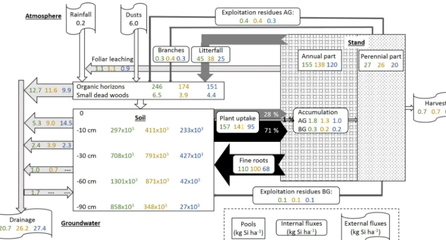
Figure 6.Summary scheme of Si cycling in plots DC, EC and RL at our study forest site, including (i) pools of Si in the biomass, (ii) internal Si fluxes, i.e. in the soil–plant system, (iii) external Si fluxes entering or leaving the soil–plant system and (iv) the DSi budget in the different layers of the ecosystem. Pools are presented by rectangular boxes (tree annual and perennial parts, organic horizons and small dead wood, and soil). Internal fluxes (solid form from the tree to the soil, i.e. fine roots, litterfall including leaves, buds and branches, and exploitation residues; and in solution from the soil to the plant, i.e. the tree uptake) are presented in boxes with rounded edges. Grey/black arrows indicate the direction and the intensity of the internal fluxes. The external fluxes (inputs: rainfall and dust deposits, and outputs: drainage and biomass harvest) are presented in flag boxes. For each pool and flux, values presented are those of the plots DC (in green), EC (in orange) and RL (in blue). The DSi budget in the different layers (forest floor and different soil layers) are represented with white arrows, which indicate the direction and the intensity of the fluxes. Arrows leaving the layer indicate the production of DSi in this layer. In contrast, arrows entering the layer indicate the immobilization of DSi in this layer. Values presented in each box and arrow are annual mean values for plots DC, EC and RL (except for atmosphere values which are similar for the three plots). The AG and BG correspond to above-ground and below-ground tree compartments.
mineral precipitation, induced by a decrease in Si drainage with depth, as observed by Sommer et al. (2013).
The Si produced in the soils was mainly leached out of the soil profile by drainage during winter. The an-nual drainage flux ranged from 21 to 27 kg Si ha−1yr−1 in the three soils at the Montiers site, which is higher than those measured in other beech forests by Bartoli (1983; 0 kg Si ha−1yr−1), Cornelis et al. (2010b; 6 kg Si ha−1yr−1), Sommer et al. (2013; 14 kg Si ha−1yr−1) and Clymans et al. (2011; 18 kg Si ha−1yr−1). The differences can result from multiple factors, i.e. topography, soil properties (tex-ture, struc(tex-ture, pH), rainfall (level and intensity) and other climatic factors, and stand characteristics (tree species and age, stem density, ground vegetal cover, etc.). In our study, the Si leached out of the soil profile was negligible compared to the Si taken up by trees, i.e. ratios of 1:4 and 1:7 in RL and DC. If we deduce the part of Si that was leached from the organic horizons, these ratios rise to about 1:5 and 1:22 in RL and DC. Because BSi in general is more soluble than lithogenic or pedogenic Si (Fraysse et al., 2009; Cornelis and Delvaux, 2016), very little of the Si leached within the soil
profile directly results from the dissolution of soil minerals, as demonstrated in other studies in temperate forests (Bar-toli, 1983; Watteau and Villemin, 2001; Gérard et al., 2008; Cornelis et al., 2010a, 2011; Sommer et al., 2006, 2013). 4.4 Si cycle at stand scale
Silicon inputs and outputs have minor contributions to the Si budget in our forest ecosystem, and the Si cycle is mainly driven by internal fluxes, especially recycling of BSi. How-ever, Struyf et al. (2010) observed that land use is the most important controlling factor of Si mobilization in European watersheds. These authors showed that deforestation and conversion to agricultural land or other land uses lead to a 2-fold to 3-2-fold decrease in baseflow delivery of Si.
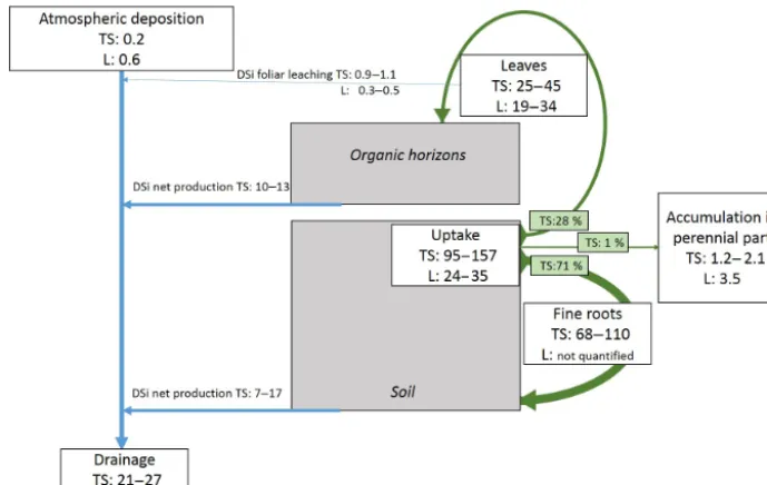
Figure 7.Summary scheme of the main findings of this study (TS) and comparison with other studies (L; Bartoli, 1983; Cornelis et al., 2010a; Sommer et al., 2013). The Si stocks and fluxes are in kg ha−1of Si.
in the perennial tree compartments returned each year to the soil via branch falls and exploitation residues (<7 cm diam-eter branches left on the floor and small/coarse roots left in the soil) and approximately 40 % was exported out of the site (stem and >7 cm diameter branches). As a result, the amount of Si immobilized in trees remained almost constant over time at the stand scale (mean Si immobilization for the three plots, 0.1 kg ha−1yr−1).
In the organic horizons and in the soil, mainly in the 0– 10 cm layer, we observed a high net Si production, likely resulting from the decomposition of litter leaves and testate amoebae in the organic horizons and of fine roots in the soil (Fig. 6). The seasonal dynamics of net Si production dur-ing the year suggests a relationship between biological activ-ities and Si production, i.e. high net Si production at the end of the summer linked to fine-root decomposition and lower net Si production during spring/summer induced by tree up-take. Net Si production decreased with depth, and an immo-bilization of Si was observed in the deeper soil layer in plot DC (Fig. 6). This likely resulted from both a decrease in Si production (less root and clay) and the precipitation of Si through the formation of secondary minerals, resulting from reduced drainage flux.
The assessment of Si pools and fluxes in the different com-partments of our forest ecosystem coupled with a seasonal dynamic follow-up reveal a rapid and almost total recycling of the Si at the stand scale and underline the key-role of bio-logical processes, mainly fine roots, in the Si cycle.
4.5 Soil influence in the soil Si inputs/outputs
eco-logical significance by protecting plants against herbivores and phytopathogens (Currie and Perry, 2007; Lins et al., 2002). The variations in Si content in the annual tree com-partments induced by the soil type significantly affected the Si fluxes in the ecosystem. The annual uptake and Si re-cycling (leaves and buds, beechnuts, fruit capsules and fine roots) were 127.2 and 154.0 kg ha−1in plot DC, as opposed to 94.8 and 92.7 kg ha−1in plot RL.
In return, the bound solutions were more concentrated in Si in plot RL compared to in plot DC. This is partly due to the higher clay content in plot RL compared to in plot DC (clay was 2 times higher in plot RL). This considerably in-creases the specific surface area of minerals and improves their weatherability and water retention capacity (Carroll and Starkey, 1971; Petersen et al., 1996).
5 Conclusion
By coupling different approaches (annual budget in solid vegetal and solution phases and monthly dynamics of solu-tions) and methods (direct in situ measurements and standard and site-specific modelling) to quantify Si pools and fluxes in the different ecosystem compartments, our study allowed us to assess the Si cycle at the forest stand scale. Interestingly, our study highlights the main contribution of fine roots and, to a lesser extent, of leaves in the Si cycle (Fig. 7). Almost all the DSi was taken up by trees at any given time (very weak leaching out of the soil profile) and was recycled each year (approximately 99 %, only 1 % accumulated in peren-nial tissues). This suggests that the Si cycle is almost closed during the vegetation period: DSi is taken up by vegetation, then Si is returned to the soil mainly through root and leave decomposition in the form of DSi, which is again taken up by vegetation. This observation is consistent with that of Som-mer et al. (2013), who demonstrated a low contribution of geochemical weathering processes to the Si cycle in a forest biogeosystem on a decadal timescale. The seasonal dynamics of DSi confirmed the key role of biological processes in the Si cycle, notably through the massive production of DSi dur-ing the decomposition of fine roots. Our study also revealed that soil type influences the Si accumulation in trees and the Si production in the soil. Trees accumulated more Si when developed on a Si-richer soil such as DC, resulting in higher Si recycling (factor of 1.6). While Si release was relatively similar in the organic horizons for the three plots, its produc-tion in the soil, mainly in the 0–10 cm layer, was twice as high in plot RL and richer in clays than in plot DC.
Further research is needed in the medium term (i) to assess the mineralization speed of fine roots in the soil and the speed of transformation of the root BSi into DSi; (ii) to determine the annual and seasonal fates of the DSi issued from roots be-tween uptake, mineral precipitation, drainage and fixation by organisms; and (iii) to quantify the vertical transfer of solid particulates between organic horizons and topsoil.
Data availability. Some underlying data can be accessed in the Supplement (Figs. S1 and S2).
Supplement. The supplement related to this article is available online at: https://doi.org/10.5194/bg-15-2231-2018-supplement.
Competing interests. The authors declare that they have no conflict of interest.
Acknowledgements. We acknowledge Serge Didier for site implementation and management; Laurent Saint-André, Laura Franoux and Astrid Genêt for the development of allometric equations; Claire Pantigny, Louisette Gelhaye, Bruno Simon, Claude Nys, Jonathan Mangin, Céline Goldstein, Frédérique César, Maëlle D’Arbaumont and Maxime Simon for technical help; Lise Salsi, for preparing the samples and performing the SEM and EDX analyses; the National Forest Office (ONF) for welcoming our experimental site in the domanial forest of Montiers and for the stand management and American Journal Experts; and Krista Bateman for reviewing the English of the paper, as well as the reviewers who have, through their suggestions, significantly improved the quality of the manuscript. The authors acknowledge the facilities of the French National Institute for Agricultural Research and the Service d’Analyse des Roches et des Minéraux of the French National Center for Scientific Research. This work was supported by the Andra and INRA (accord spécifique no. 9) and GIP-Ecofor (contract no. 1138451B).
Edited by: Michael Bahn
Reviewed by: Eric Struyf and one anonymous referee
References
Alexandre, A., Meunier, J. D., Colin, F., and Koud, J. M.: Plant impact on the biogeochemical cycle of silicon and related weath-ering processes, Geochim. Cosmochim. Ac., 61, 677–682, 1997. Alexandre, A., Bouvet, M., and Abbadie, L.: The role of savannas in the terrestrial Si cycle: a case study from Lamto, Ivory Coast, Global Planet. Change, 78, 162–169, 2011.
Bakker, M. R., Turpault, M. P., Huet, S., and Nys, C.: Root distribu-tion ofFagus sylvaticain a chronosequence in western France, J. Forest Res., 13, 176–184, 2008.
Bartoli, F.: The biogeochemical cycle of silicon in two temperate forest ecosystems, Ecol. Bull., 35, 469–476, 1983.
Bartoli, F. and Souchier, B.: Cycle et rôle du silicium d’origine végétale dans les écosystèmes forestiers tempérés, Ann. Sci. For-est., 35, 187–202, 1978.
Bauer, P., Elbaum, R., and Weiss, I. M.: Calcium and silicon min-eralization in land plants: transport, structure and function, Plant Sci., 180, 746–756, 2011.
Bolte, A. and Villanueva, I.: Interspecific competition impacts on the morphology and distribution of fine roots in European beech (Fagus sylvaticaL.) and Norway spruce (Picea abies(L.) Karst.), Eur. J. For. Res., 125, 15–26, 2006.
Brunner, I., Bakker, M. R., Björk, R. G., Hirano, Y., Lukac, M., Aranda, X., Børja, I., Eldhuset, T. D., Helmisaari, H. S., Jour-dan, C., Konôpka, B., Miguel Pérez, C., Persson, H., and Osto-nen, I.: Fine-root turnover rates of European forests revisited: an analysis of data from sequential coring and ingrowth cores, Plant Soil, 362, 357–372, 2013.
Calvaruso, C., Kirchen, G., Saint-André L., Redon, P.-O., and Tur-pault, M.-P.: Relationship between soil nutritive resources and the growth and mineral nutrition of a beech (Fagus sylvatica) stand along a soil sequence, Catena, 155, 156–169, 2017. Carroll, D. and Starkey, H. C.: Reactivity of clay minerals with acids
and alkalies, Clay. Clay Miner., 19, 321–333, 1971.
Claus, A. and George, E.: Effect of stand age on fine-root biomass and biomass distribution in three European forest chronose-quences, Can. J. Forest Res., 35, 1617–1625, 2005.
Clymans, W., Struyf, E., Govers, G., Vandevenne, F., and Conley, D. J.: Anthropogenic impact on amorphous sil-ica pools in temperate soils, Biogeosciences, 8, 2281–2293, https://doi.org/10.5194/bg-8-2281-2011, 2011.
Conley, D. J.: Terrestrial ecosystems and the global biogeochemical silica cycle, Global Biogeochem. Cy., 16, 1–8, 2002.
Cornelis, J. T. and Delvaux, B.: Soil processes drive the biological silicon feedback loop, Funct. Ecol., 30, 1298–1310, 2016. Cornelis, J. T., Ranger, J., Iserentant, A., and Delvaux, B.: Tree
species impact the terrestrial cycle of silicon through various up-takes, Biogeochemistry, 97, 231–245, 2010a.
Cornelis, J. T., Delvaux, B., Cardinal, D., Andre, L., Ranger, J., and Opfergelt, S.: Tracing mechanisms controlling the release of dis-solved silicon in forest soil solutions using Si isotopes and Ge/Si ratios, Geochim. Cosmochim. Ac., 74, 3913–3924, 2010b. Cornelis, J. T., Titeux, H., Ranger, J., and Delvaux, B.: Identification
and distribution of the readily soluble silicon pool in a temperate forest below three distinct tree species, Plant Soil, 342, 369–378, 2011.
Currie, H. A. and Perry, C. C.: Silica in plants: biological, biochem-ical and chembiochem-ical studies, Ann. Bot.-London, 100, 1383–1389, 2007.
Dahlgren, R. A. and Ugolini, F. C.: Effects of tephra addition on soil processes of spodosols in the Cascade Range, Washington, USA, Geoderma, 45, 331–335, 1989.
Emsens, W. J., Schoelynck, J., Grootjans, A. P., Struyf, E., and Van Diggelen, R.: Eutrophication alters Si cycling and litter decom-position in wetlands, Biogeochemistry, 130, 289–299, 2016. Epstein, E.: Silicon, Annu. Rev. Plant Phys., 50, 641–664, 1999. FAO: World Reference Base for Soil Resources 2014, in: World Soil
Resources Report 106, FAO, Rome, 1–192, 2016.
Finér, L., Ohashib, M., Noguchic, K., and Hiranod, Y.: Factors caus-ing variation in fine root biomass in forest ecosystems, Forest Ecol. Mangag., 261, 265–277, 2011.
Fishkis, O., Ingwersen, J., Lamers, M., Denysenko, D., and Streck, T.: Phytolith transport in soil: a field study using fluo-rescent labelling, Geoderma, 157, 27–36, 2010.
Fraysse, F., Pokrovsky, O. S., Schott, J., and Meunier, J. D.: Surface chemistry and reactivity of plant phytoliths in aqueous solutions, Chem. Geol., 258, 197–206, 2009.
Gal, A., Brumfeld, V., Weiner, S., Addadi, L., and Oron, D.: Certain biominerals in leaves function as light scatterers, Adv. Mater., 24, 77–83, 2012.
Gaul, D., Hertel, D., and Leuschner, C.: Estimating fine root longevity in a temperate Norway spruce forest using three in-dependent methods, Funct. Plant Biol., 36, 11–19, 2009. Gérard, F., Mayer, K. U., Hodson, M. J., and Ranger, J.: Modelling
the biogeochemical cycle of silicon in soils: application to a tem-perate forest ecosystem, Geochim. Cosmochim. Ac., 72, 741– 758, 2008.
Granier, A., Bréda, N., Biron, P., and Villette, S.: A lumped wa-ter balance model to evaluate duration and intensity of drought constraints in forest stands, Ecol. Model., 116, 269–283, 1999. Harter, T., Wagner, S., and Atwill, E. R.: Colloid transport and
filtra-tion ofCryptosporidium parvumin sandy soils and aquifer sedi-ments, Environ. Sci. Technol., 34, 62–70, 2000.
Heineman, K. D., Turner, B. L., and Dalling, J. W.: Variation in wood nutrients along a tropical soil fertility gradient, New Phy-tol., 211, 440–454, 2016.
Hendriks, C. M. A. and Bianchi, F. J. J. A.: Root density and root biomass in pure and mixed forest stands of Douglas-fir and Beech, Neth. J. Agr. Sci., 43, 321–331, 1995.
Henry, M., Picard, N., Trotta, C., Manlay, R., Valentini, R., Bernoux, M., and Saint-André, L.: Estimating tree biomass of sub-Saharan African forests: a review of available allometric equations, Silva Fenn., 45, 477–569, 2011.
Hodson, M. J., White, P. J., Mead, A., and Broadley, M. R.: Phylo-genetic variation in the silicon composition of plants, Ann. Bot.-London, 96, 1027–1046, 2005.
Jones, L. H. P. and Handreck, K. A.: Studies of silica in the oat plant. III. Uptake of silica from soils by plant, Plant Soil, 23, 79–96, 1965.
Jourdan, C., Silva, E. V., Goncalves, J. L. M., Ranger, J., Mor-eira, R. M., and Laclau, J. P.: Fine root production and turnover in Brazilian Eucalyptus plantations under contrasting nitrogen fer-tilization regimes, For. Ecol. Manage., 256, 396–404, 2008. Kabata-Pendias, A. and Mukherjee, A. B.: Trace Elements from
Soil to Human, Springer, Berlin, 2007.
Kirchen, G., Calvaruso, C., Granier, A., Redon, P.-O., Van Der Hei-jden, G., Bréda, N., and Turpault, M.-P.: Local soil type variabil-ity controls the water budget and stand productivvariabil-ity in a beech forest, Forest Ecol. Mangag., 390, 89–103, 2017.
Konôpka, B.: Differences in fine root traits between Norway spruce (Picea abies (L.) Karst.) and European beech (Fagus sylvat-icaL.) – a case study in the Kysucké Beskydy Mts, J. For. Sci., 55, 556–566, 2009.
Krieger, C., Calvaruso, C., Morlot, C., Uroz, S., Salsi, L., and Turpault, M.-P.: Identification, distribution, and quantification of biominerals in a deciduous forest, Geobiology, 15, 296–310, 2017.
Lavelle, P.: Earthworm activities and the soil system, Biol. Fert. Soils, 6, 237–251, 1988.
Le Goff, N. and Ottorini, J.-M.: Root biomass and biomass incre-ment in a beech (Fagus sylvaticaL.) stand in North-East France, Ann. For. Sci., 58, 1–13, 2001.