Quartic planar graphs

(1)

Quartic planar graphs

Jane Tan

October 2018

(2)

(3)

Declaration

The work in this thesis is my own except where otherwise stated.

(4)

(5)

Acknowledgements

First, I’d like to thank my supervisors, Brendan McKay and Scott Morrison. Brendan – your guidance has been invaluable. I’m so grateful for all of the exciting problems you’ve introduced me to, and that you’re still putting up with me a full two years after you agreed to take me on “just for one semester”. And Scott – thank you for your help with editing, your calming presence, and for sharing the good chalk.

I would also like to thank all of the lecturers at the MSI who have been so generous with their time and from whom I have learnt so much. Special thanks to Vigleik, Joan and Andrew for teaching fantastic reading courses and supervising me in projects over the years.

Thanks also go to all of the honours students, even the cookie monster and the elusive north-siders. It’s been great fun sharing our shiny new office!

Last but not least, thank you to my family for always being on the phone.

(6)

(7)

Abstract

In this thesis, we explore three problems concerning quartic planar graphs. The first is on recursive structures; we prove generation theorems for several interest-ing subclasses of quartic planar graphs and their duals, buildinterest-ing on previous work which has largely been focussed on the simple or nonplanar cases. The second problem is on the existence of locally self-avoiding Eulerian circuits. As an ap-plication of a generation theorem, we prove that all but one 3-connected quartic planar graphs have an Eulerian circuit that is free of subcycles of length 3 or 4. This implies that a 3-connected quartic planar graph admits a P5-decomposition

if and only if it has even order. Finally, we give some new smaller counterex-amples to a disproven conjecture of Lov´asz on circle representations of quartic planar graphs. We also present a gluing construction that tells us a little more about the obstructions to circle representability, although a full characterisation remains elusive.

(8)

(9)

Notation

In the following, let G be an undirected graph that may have loops and parallel edges, and v be a vertex of G.

V(G) The set of vertices of G.

E(G) The multiset of edges of G.

|G| The order of G, which is |V(G)|.

G∗ The planar dual of a planar graphG.

d(v) The degree of the vertex v.

N(v) The set{w∈V(G) :vw∈E(G)} of neighbours of v. H ⊆G H is a (not necessarily induced) subgraph of G.

G[A] The subgraph of G induced byA ⊆V(G), or A⊆E(G). G−A The subgraph ofGobtained by deleting the vertices in a subset

A⊆V(G) and all incident edges.

κ(G) The vertex-connectivity of G.

λ(G) The edge-connectivity of G.

Pn The path onn vertices.

Cn The cycle on n vertices.

Kn The complete graph onn vertices.

Km,n The complete bipartite graph with colour classes consisting of

m and n vertices.

(12)

(13)

Chapter 1 Introduction

1.1 Overview

A graph is k-regular if every vertex has the same finite degree k. By cubic and

quartic, we mean 3-regular and 4-regular respectively. The former have been well-studied and exhibit many nice properties, so one naturally looks to quartic graphs for interesting extensions of those results, as well as fresh problems that pertain to properties particular to this class.

In this thesis, we explore three problems concerning quartic planar graphs. These have garnered considerable interest as they appear in a wide range of contexts, in large part because there is a nontrivial intersection between the theory of quartic graphs and planar graph theory. For instance, any drawing of a quartic graph gives rise to a quartic planar graph provided no more than two edges cross at any point, by introducing an extra vertex at each crossing. The shadows of knots and links arise in this way (see [37]). Conversely, the face-edge incidences of any planar graph can be encoded as a quartic planar graph.

By focussing on a single class of graphs, we enjoy the opportunity to get acquainted with a particular set of properties, tools and examples that we can take into a variety of problems. This means that although the problems explored may fall under different branches of graph theory, our experiences in one inform our intuition and approach to the others. This has turned out to be quite fruitful. The following highlights from each of the three main chapters are, to the best of our knowledge, all new results.

Our first goal is to provide recursive structures for some interesting subclasses of the quartic planar graphs. These are given in the form of generation theorems, which describe how the graphs in a class can be constructed from some starting

(14)

2 CHAPTER 1. INTRODUCTION

set of graphs by applying a sequence of local expansion operations. We achieve this indirectly by first finding forbidden configuration characterisations of the dual classes of quadrangulations to those that we are primarily interested in generating, and then instead working explicitly with quadrangulations. These results build on the body work on generating simple subclasses of quadrangulations [17] and quartic graphs that are possibly non-planar [27], as well as the class of arbitrary quadrangulations without any restrictions [52].

One of the main motivations for finding recursive structures is that they fa-cilitate inductive proofs. We were able to apply this approach in the context of Eulerian circuits and path decompositions. Quartic graphs are the simplest non-trivial Eulerian graphs, making them a promising starting point for problems involving Eulerian circuits. As our second problem, we consider the restricted class of Eulerian circuits that are free of short subcircuits. We show that all but one 3-connected quartic planar graphs have an Eulerian circuit that avoids 3-cycles and 4-cycles. The proof is constructive, and extends existing work on the avoidance of sub-circuits of length 3 for a similar class of graphs. As a corollary, we also show that a 3-connected quartic planar graph admits a P5-decomposition

if and only if it has even order.

The final problem is in the area of graph drawing, specifically geometric repre-sentations of graphs. Here, we consider a disproved conjecture of Lov´asz that ev-ery quartic planar graph can be represented by a system of circles in the plane. We came across this conjecture from a paper by Broersma, Duijvestijn and G¨obel [23], who identified it as a potential theoretical application of their graph generation theorem back when it was still open. That method did not work out as hoped, but it did lead us to our work geared toward understanding the obstructions to circle representability, and working toward characterising those graphs that admit a circle representation. On this path, we produce two new families of counterex-amples, and improve on the order of the smallest known counterexamples from 822 to 68.

(15)

1.2. CONVENTIONS 3

1.2 Conventions

We will assume basic familiarity with graph theory. For a refresher, we refer to Diestel [26] with a warning that we occasionally deviate from the notation and definitions used there. In this thesis, we use the following conventions.

A graph is a pair G = (V, E) such that V is a finite set, and E is a finite multiset consisting of elements of [V]2 ∪ {(v, v)| v ∈ V} where [V]2 denotes the set of all 2-element subsets of V. An edge that has both endvertices being the same vertex is called a loop, and two edges are said to be parallel if they have the same endvertices. By this definition, our graphs are assumed to be finite, undirected, and unless otherwise indicated may have loops and parallel edges. In addition, we will assume that our graphs are connected unless otherwise indicated. We say that an edge isincident to its endvertices, and vice versa. Two vertices are adjacent if there is an edge between them, meaning incident to them both. The degree of a vertex v, denoted by d(v) is the number of edges incident to v, with loops counted twice. If an edge e is not parallel to any other edges, we say that e is simple. A simple graph is then a graph that is loopless and in which every edge is simple. We sometimes use the term multigraph to emphasise that loops and the parallel edges may be present, but this should be read no differently than ‘graph’ as we have defined it above.∗ We refer to any subgraph consisting of only two parallel edges and their endvertices as a digon.

A walk of length k between v0 and vk in a graphGis an alternating sequence

of vertices and edges v0e0v1e1. . . ek−1vk, where each two consecutive objects are

incident. Here, v0 and vk are endvertices of the path, whilst vi for 1≤i≤k−1

are the inner vertices. Walks are not directed, but it is convenient to say that they ‘start’ and ‘end’ at particular vertices so we will frequently do so.

There are a few different notations to denote walks that we shall use depending on context. For simple graphs, since each edge is uniquely identified by its endver-tices it is enough to write down the sequence of verendver-tices in the formv0v1. . . vk, so

that the implicit sequence of edges is v0v1, v1v2, . . . , vk−1vk. Long walks, such as

those in Chapter 4, are sometimes abbreviated to a form such as v0Xvk in which

X represents the walk v1. . . vk−1 where v0 is adjacent to v1 and vk−1 is adjacent

to vk. When parallel edges exist, we must be careful to distinguish which edge

we are taking between two vertices. In that case we include the edge names as well. For sake of readability we adopt the formatv0

e0

—v1 e1

—v2. . . vk−1 ek−1

—vk, which

∗_{The term}_multigraph _(also,_pseudograph_{) is sometimes used to denote what we are calling}

(16)

4 CHAPTER 1. INTRODUCTION

we will see regularly in Chapter 3.

We say that a walk isclosed if its final vertex is the same as its initial vertex, and open otherwise. Acircuit is then a closed walk of length at least 2 in which each edge occurs at most once. An Eulerian circuit is a circuit in which every edge is traversed precisely once. A walk in which each vertex occurs at most once (hence each edge also appears at most once), except possibly where the initial vertex is the same as the last, is called apath, and a closed path of length at least two is called a cycle. A cycle with an even number of edges is an even cycle, and

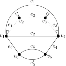
odd otherwise. We use the term digon to refer to a cycle of length 2.

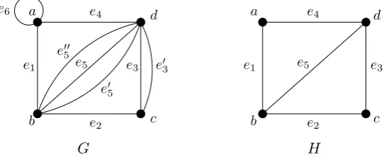
Example 1.1. Two graphs are shown in Figure 1.1. The first graph, G, is not simple because e6 is a loop, e3 is parallel toe30, and e5, e05 and e

00

5 are all parallel.

The walkd—ce3 e 0

3

—d—ae4 —ae6 —be1 —ce2 —de3 is closed but not a circuit sincee3is repeated,

and it contains a circuit d—ae4 —ae6 —be1 —ce2 —de3 that is not a cycle sinceais repeated. The walk be5de05b is a digon, as is be005de05b.

On the other hand, H is a simple graph. The cycle ae1be2ce3de4a can be

abbreviated toabcda. An example of a closed walk that is not a circuit isabdcba.

d a

b c

e4

e1

e2

e0₃ e3

e5

e00₅

e05

e6

G

d a

b c

e4

e1

e2

e3

e5

[image:16.595.136.407.417.528.2]

H

Figure 1.1: A graph and a simple graph.

(17)

Chapter 2 Toolkit

In this chapter, we record some standard results and constructions in graph the-ory, as well as properties specific to quartic planar graphs and the closely related class of quadrangulations. These results are mostly classical, to the extent that their proofs in literature tend to be omitted or else invoke folklore∗. In those cases, we supply a short proof or reference.

2.1 Plane and planar graphs

Definition 2.1. An embedding of a graph G in the plane is an injective map that sends V(G) to points in the plane and edges of E(G) to disjoint simple open arcs such that the image of each edge joins the images of its endvertices.

Such an embedding corresponds to a drawing of the graph in the plane so that there are no edge crossings. The leads to the following terms that we should be careful to distinguish.

Definition 2.2. A graph is planar if it has an embedding into the plane. The image is called a plane graph, which contains the data of an abstract graph together with a specified embedding.

The faces of a plane graph G are the maximal connected subsets of the open set_R2₋_{G. Note that each of these is homeomorphic to an open disk, so we say}

that this is a cellular embedding. This is automatic for connected graphs drawn on the plane, but not necessarily so if we embed graphs on other surfaces. The topological boundary of any face corresponds to a walk in the graph, and we say

∗_{This is quoted from the proof of Lemma 1 in [17].}

(18)

6 CHAPTER 2. TOOLKIT

that the face is incident to each of the edges and vertices in its boundary. More generally, by the Jordan Curve Theorem, any cycle in a graph bounds exactly two regions. There is always one unbounded face which we call the outer face, and similarly one unbounded region which we call the outer region or exterior, as opposed to inner regions and interior of a cycle. If at least one of the regions bounded by a particular cycle is also a face, then we say that the cycle is facial, otherwise it is non-facial orseparating.

Remark 2.3. Having an embedding in the plane is equivalent to having an embedding in the sphere S2_{, since this is the one point compactification of the}

plane. Given an embedding of a graph on the sphere, we may assume without loss of generality that no part of the graph lies on the north pole by possibly rotating. The stereographic projection then gives a correspondence between spherical and planar embeddings.

One should think of the difference as being that a planar embedding comes with a particular choice of outer face, which corresponds on the sphere to the face that contains the north pole. We will freely switch between these two perspectives, as although our diagrams must necessarily be planar, it is advantageous to think of our graphs as being on the sphere since this means all faces are treated equally.

In practice, when we fix an embedding on the plane as opposed to the sphere, the only difference is that the planar embedding comes with a choice of outer face so it then makes sense to refer to the interior and exterior regions of any cycle. This is useful, for instance, in the following situation.

Lemma 2.4. A plane graph G for which every face is bounded by a walk of even length is bipartite.

(19)

2.1. PLANE AND PLANAR GRAPHS 7

The plane graphs in which every face is bounded by a walk of the same even length form a special class of graphs that satisfy the conditions of the previous lemma. More generally:

Definition 2.5. A k-angulation (of the sphere) is a plane graph in which every face is bounded by a walk of length k for k ≥3.

The 3-, 4- and 5-angulations are called triangulations, quadrangulations and pentangulations respectively.

Corollary 2.6. Quadrangulations are bipartite.

Provisionally, we say that two plane graphs are equivalent if they are related by a homeomorphism of the sphere that restricts to an isomorphism of graphs, and regard an embedding as an equivalence class. Observe that a graph embedded on the plane can be transformed into an equivalent one with a different choice of outer face by applying a M¨obius transformation. A second equivalent definition will be given once we introduce combinatorial embeddings. It is certainly possible for a graph to have inequivalent embeddings. An example is shown in Figure 2.1.

Figure 2.1: Three planar embeddings of a planar graph; the first is equivalent to the third but not to the second.

There are two famous characterisations of simple planar graphs. Recall that

subdividing an edge in a graph means to replace the edge by a path between its endvertices such that each inner vertex has degree 2. An edge contraction is per-formed by removing an edge xy together with all incident edges, and identifying x andy into a new vertex that is incident to all of the edges formerly incident to xory. It is implicit that any new parallel edges created are also merged. A graph G0 is a subdivision of G if it can be obtained by subdividing edges of G, and it is aminor of G if it can be constructed from G by a series of edge contractions, vertex deletions and edge deletions. An example is shown in Figure 2.2.

Theorem 2.7 (Kuratowski). A simple graph is planar if and only if does not contain a subdivision isomorphic to K5 or K3,3.

(20)

F G H

Figure 2.2: The graph F contains G as a minor and a subdivision ofH.

The following result of Euler is classical. For now, we only state the simplest version for the plane.

Theorem 2.9 (Euler’s formula). For any plane graph with n vertices, e edges and f faces,

n−e+f = 2.

Since the number of faces is determined by the number of edges and vertices, we can refer to the number of faces of a planar (rather than plane) graph as a well-defined quantity. Typically, Euler’s formula is applied to show that certain graphs are non-planar, or to obtain bounds on the number of vertices, edges or faces given some relationships between these values. For example, the following is standard.

Proposition 2.10. There are no simple planar k-regular graphs for k ≥6. Proof. LetGbe any simple planar graph withnvertices,eedges andf faces. We may assume thatv ≥3 ande≥3, so each face is bounded by at least three edges. Then 3f ≤2e. Substituting this into Euler’s formula gives 2e−3e ≥6−3n and hence 2e ≤ 6n −12. Diving through by n, we find that the average degree is at most 6− 12

n which is strictly less than 6. Therefore, G must have a vertex of

degree at most 5.

(21)

Figure 2.3: A non-cellular embedding of a graph on the torus.

Theorem 2.11 (Euler’s formula). For any graph with n vertices, e edges and f

faces embedded on a surface Σ,

n−e+f =

  

2−2g, if Σ is orientable with genus g,

2−h, if Σ is non-orientable with genus h.

2.1.1 Combinatorial embeddings

The definition we have so far of an embedding is specifically a topological em-bedding. There is also a purely combinatorial definition, which is often more convenient to work with.

Definition 2.12. A rotation at a vertex in a map is the cyclic ordering of edges incident to that vertex induced by a specified orientation. A rotation system for a graph consists of a choice of rotation at each vertex.

There is a one-to-one correspondence between cellular embeddings on ori-entable surfaces and the possible rotation systems of a graph, a fact which is sometimes called the Heffter-Edmonds-Ringel rotation principle [61]. That is, any cellular embedding of a plane graph gives rise to a unique rotation system, and conversely specifying the cyclic order at each vertex determines a cellular embedding of the graph into some orientable surface. For the proof of this corre-spondence, we refer the reader to [39, 61].

(22)

There is also a twisted version of a rotation system that can be used to encode graphs embedded on non-orientable surfaces which is detailed in [39, 61].

The following notion of equivalence for combinatorial embeddings corresponds to our earlier topological definition.

Definition 2.13. Two maps are regarded as equivalent if they are related by an isomorphism of abstract graphs that also either preserves the cyclic ordering of edges at each vertex, or reverses the ordering at every vertex.

2.1.2 Dual, medial and radial graph constructions

We now record several related constructions on plane graphs that encode infor-mation about the incidences between vertices, edges and faces. Recall that by default, we assume that all graphs are connected.

Planar duals

To each planar graph G, we can associate another planar graphG∗ called itsdual

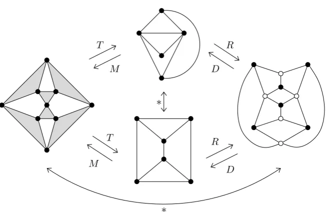
as follows. Place a vertex in each face of G, so V(G∗) is the set of faces of G. For each edge e in G, create an edge e∗ in E(G∗) that crosses e with endvertices corresponding to the two faces adjacent to e. If e is only adjacent to only one face, then we get a loop in the dual graph. Evidently, the dual of a quartic plane graph is a quadrangulation.

Since abstract planar graphs may have inequivalent embeddings, a planar graph can have nonisomorphic duals. However, it is true that each plane graph has a unique dual. This means that a class C of plane graphs is in bijective correspondence to the dual class C∗ _:=_{G∗ _|_G_{∈ C}.}

The construction we have described is of the geometric dual graph. There is a separate notion of combinatorial dual which has quite a different description but is equivalent.

Medial graphs

(23)

In fact, every 4-regular plane graph is the medial graph M G of some plane graph G. We call the associated graph a Tait graph, as this construction was originally used by Tait in the study of knots and links. The proof is by con-struction. Given a quartic plane graph G, create a checkerboard colouring of its faces with two colours, say black and white, so that each edge is incident to one black face and one white face. Let us specify that the outer face is white. This is possible since Gis Eulerian, so G∗ is bipartite by Lemma 2.4 and a proper 2-vertex-colouring ofG∗translates to the desired checkerboard colouring ofG. Now letV(T G) correspond to the black faces, and the edge set consist ofxywhenever the faces corresponding toxandy share a vertex. Choosing the white faces gives (T G)∗, which also satisfies M T G∼G. These are the only two embedded graphs up to isomorphism that have G as their medial graph.

Radial graphs

Given a plane graphG, we define the radial graphRGto be the quadrangulation (M G)∗. This can also be constructed directly. Let V(RG) be the vertices and faces of G, with an edge xy ∈ E(RG) whenever x and y correspond to a vertex and one of its incident faces, counting multiplicities. Evidently, the radial graph encodes vertex-face incidences of G.

Conversely, from each quadrangulation we can construct a graphDGby prop-erly colouring the vertices ofGwith two colours, which is possible by Lemma 2.6, and taking the vertices of one colour class as V(DG). Two vertices are adjacent whenever they lie on the same face ofG. Again, using the other colour class gives (DG)∗ which has the same radial graphG as DG. There does not appear to be a standard name for this construction, so we use D for “diagonal” since the new edges are diagonals of the quadrangular faces of G.

(24)

M T

D R

∗

[image:24.595.114.440.95.307.2]

∗

Figure 2.4: Dual plane graphs in the centre, together with their medial graph on the left and their radial graph on the right.

2.2 A note on interpreting diagrams

Although planar graphs, by definition, are a nice class of graphs to draw, in the wild we almost never have the luxury of seeing the entire graph. Rather, it is common to work locally in small neighbourhoods of a graph at a time, but also have some knowledge about where the rest of the graph lies in terms of rotations at particular vertices. This poses some challenges when we wish to display such information precisely using diagrams.

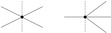
The pictures in this thesis all represent plane (embedded) graphs, and so the cyclic ordering of edges at each vertex is important. It should be noted that the embedding shown may not be the unique possible embedding, but this will be made clear whenever it is important. To represent general structures diagrammatically, we adopt a system of edge placeholders consisting of half-edges, black triangles and white triangles which may be interpreted according to the following rules.

(i) All vertices shown are distinct from each other.

(ii) Edges and half-edges (which indicate an edge must be present but one end-vertex is not depicted) occur in the cyclic order in which they are shown at each vertex.

(25)

2.3. CONNECTIVITY 13

(iv) A white triangle with an extra half-edge at a vertex indicates that at least one edge is present in this position. A bounded region containing this placeholder cannot be a facial.

(v) For any given region that contains black triangles at each incident vertex, that region must not be a face of the graph; in other words, at least one of those black triangles associated with the particular region is actually realised as one or more edges.

(vi) Any two edges that are shown consecutively in the cyclic order (not sepa-rated by any edge placeholder) at a vertex must follow each other directly in the cyclic ordering at that vertex. If a region contains no edge placeholders, then it is necessarily facial.

By convention, facial cycles will be written clockwise except the outside face which will be written anticlockwise.

v w x y

Figure 2.5: Applying the above conventions, the left digon is non-facial due to the black triangles on the inside and half-edges on the outside, whereas the right digon is facial since there is no placeholder inside the parallel edges. The region bounded outside is not a face because one of the white triangles has a half-edge.

2.3 Connectivity

Recall that a non-empty graph is connected if there is a path between any two of its vertices, and disconnected otherwise, in which case we refer to the maximal connected subgraphs as components.

Definition 2.14. A k-vertex-cutset (or k-vertex-cut) in a graph G is subset S ⊆ V(G) with |S| = k such that G−S is disconnected. The unique element in any 1-vertex-cut is called a cutvertex of the graph. A k-edge-cutset (or k-edge-cut) in a graph G is a subset T ⊆ E(G) with |T| = k such that G−T is disconnected. The unique element in any 1-edge-cut is called a bridge.

(26)

The greatest integerk such that a graphGisk-vertex-connected is thevertex connectivity of G, denoted by κ(G). Similarly, the greatest integer k such that a graph G is k-edge-connected is the edge connectivity of G, denoted by λ(G). When there is little chance of confusion, we sometimes drop the ‘vertex’ part of the above terms and just write, for example, k-connected to mean k-vertex-connected.

This definition measures how connected a graph is by how hard it is to dis-connect. In some ways, Menger’s theorem provides a more intuitive description.

Theorem 2.16 (Menger). A graph is k-edge-connected if and only if there are

k edge-disjoint paths between any two vertices. Similarly, a graph is k -vertex-connected if and only if there are k internally vertex-disjoint paths between any two vertices.

Planar graphs with sufficiently high connectivity have several nice features.

Proposition 2.17. A simple plane graph other than K1 and K2 is

2-vertex-connected if and only if every face is bounded by a cycle.

Proof. See 4.2.6 in [26].

Lemma 2.18. Every 3-vertex-connected quadrangulation is simple.

Proof. Quadrangulations are bipartite by Lemma 2.6, and hence loopless. By definition they cannot have facial digons, so if any parallel edges exist, their endvertices would form a 2-cut.

Theorem 2.19 (Whitney). The 3-connected planar graphs have unique embed-dings on the sphere.

The last theorem provides a reason for why 3-vertex-connected planar graphs are of special interest, and imposing this condition gives a further refinement of the quartic planar graphs that makes for a good entry point when approaching difficult problems.

There is one other type of connectivity that we will meet.

(27)

Equivalently, a graphGis exactly cyclicallyk-edge-connected if it is cyclically k-edge-connected but not cyclically (k+1)-edge-connected. Interest in cyclic con-nectivity arose in connection to the 4-colour theorem, with one famous reduction due to Birkhoff being that it is sufficient to prove the 4-colour theorem for exactly cyclically 5-connected planar graphs [69].

These notions of connectivity are interdependent. Being 1-vertex-connected, 1-edge-connected or connected are equivalent. It is straightforward to see that any graph with ak-edge-cutset also has ak-vertex cutset by taking one endvertex of each of the edges in the cut. This means that if G is k-vertex-connected then it is also k-edge-connected. That is, for any non-trivial graph G we have κ(G)≤ λ(G) ≤δ(G) where δ(G) is used here to denote the minimum degree of any vertex inG. Similarly, a graph that is cyclically k-edge-connected is k-edge-connected. The following is another easy deduction.

Proposition 2.21. If G is cubic, then κ(G) =λ(G).

Further relationships exist for planar graphs. One that will be useful for us when we later consider generating triangulations is:

Proposition 2.22. A triangulation is n-vertex-connected if and only if its dual is cyclically n-edge-connected.

2.3.1 Cuts in quartic planar graphs

From the construction described earlier it is clear the dual of a simple graph need not be simple, and the reason for this is secretly encoded in edge-cutsets. The following classical result makes this precise.

Lemma 2.23 (Cut-cycle duality). If G is a connected plane graph, there is a one-to-one correspondence between cycles of G and minimal edge-cutsets of G∗.

(28)

The following is an immediate but noteworthy consequence.

Proposition 2.24. There are no cuts consisting of an odd numbers of edges in a quartic planar graph.

Proof. We saw in Lemma 2.6 that quadrangulations of the sphere are bipartite, and hence do not have any odd cycles. Therefore their duals, which are quartic plane graphs, do not have odd cutsets by Lemma 2.23. It follows that this is also true of quartic planar graphs by choosing any planar embedding.

For quartic plane graphs, we can also say very explicitly what 1-vertex-cuts and 2-vertex-cuts look like. This is useful in cases where we would like to de-compose a graph into blocks that have higher connectivity than the whole graph in order to apply some property that normally required 3-vertex-connectedness. The characterisation tells us how blocks might be joined together.

[image:28.595.180.370.483.540.2]

Let G be a quartic planar graph with a cutvertex v. This cut can only take one of two forms, as shown in Figure 2.6, corresponding to the situations where v is adjacent to two edges in each component ofG∗−v, or three in one component and one in the other. If the configuration on the right of Figure 2.6 is present, then since G∗ is quartic, each component ofG∗−v has an odd number of vertices with odd degree which is impossible. Thus, any 1-cut takes the left configuration.

Figure 2.6: Possible 1-cut configurations

(29)

the right, in which case y has one on the left and three on the right, or 3 on the left and one on the right. These are all the possibilities up to symmetry.

We will typically represent these as shown in Figure 2.7, where the shaded regions represents the sides of the cut. The endvertices of the half-edges shown may not be distinct. The top row are balanced cuts whilst the other three are

unbalanced. Observe that the unbalanced 2-cuts are all related; the first one can be seen as a special case of the second, and any graph that has the second type of 2-cut must also have the third and vice versa by replacing one of the cut vertices with its unique neighbour on one side of the cut.

(30)

(31)

Chapter 3 Recursive generation

Informally, the idea of generating a class of graphs is that starting with a subclass of basic graphs which are in some way simpler, we can recursively apply local expansion operations to gradually increase their complexity, as measured by some parameter. The superclass of graphs that can be obtained in this manner is said to be generated from the starting set, and the corresponding result is ageneration theorem for the larger class.

Apart from being insightful structural results, the appeal of having such de-scriptions for particular classes of graphs stems from two main applications. First, generation theorems facilitate inductive proofs. If one can show that some prop-erty is satisfied by the starting graphs and preserved by the expansion operations, then it would follow that it is also satisfied by graphs in the superclass. The second application is to practical graph generators, where implementations of the theo-rem make it possible to enumerate the graphs in the class (up to some parameter) and – in contrast to theoretical enumeration – output an exhaustive list. This is useful for checking conjectures, and also has applications to chemistry where certain molecular structures can be generated (see for instance [15, 16, 35, 40]).

The main result in this chapter is a collection of generation theorems of quad-rangulations and their dual classes of quartic graphs, together with the proof of those dual relationships. In light of these characterisations of the dual classes, we will instead explicitly be generating quadrangulations as we find this to be a more convenient setting in which to work. We will begin with a more abstract discus-sion of recursive generation, and familiarise ourselves with generation theorems for some closely related classes of graphs.

(32)

20 CHAPTER 3. RECURSIVE GENERATION

3.1 Definitions and literature

The following key definition formalises our earlier description of what it means to recursively generate a class of graphs.

Definition 3.1. Given a class of graphs Y and a subclass X together with a set of operations, we say that the class Y can be generated from class X by those operations if for every graph in G ∈ Y there exists a sequence of graphs G0, G1, . . . , Gn =G such that G0 ∈X, Gi ∈ Y for each 1≤i ≤n and Gi+1 can

be obtained from Gi by applying one of the operations.

That is, one can obtain any graph in Y by recursively applying operations starting with some graph in X. We are specifically interested in those operations that increase some parameter related to the graph. Some common possibilities here include the number of vertices, edges or faces, as well as possibly multigraph structures. These operations are typically called expansions, so accordingly their inverses are reductions. Note that the class we are generating need not be closed under the set of expansion operations, but it is important that after applying a reduction to any graph in the class, the resulting graph is still in the class.

With a view to practical applications, there are some general qualities that we like to have in a generation theorem. It is usually the case that the starting class of graphs to either be a small finite collection graphs, or else some infinite family for which there is a general, explicit description such as the cycles, prisms, or pseudo-double wheels. It is also common for generation theorems to build upon others. For instance, if we know how to generate some class B of graphs from A, then it may be convenient to start with B to generate some larger superclass C. Of course, this could then be phrased as a statement generating C from A by simply concatenating the lists of operations. Regarding choice of expansion operations, it is generally desirable to have as few operations as possible, and with each one being as restricted as possible, meaning those for which the inverse reduction operations can be applied in fewer places are considered more efficient.

Other methods of practical generation

(33)

3.1. DEFINITIONS AND LITERATURE 21

has only one edge, sayac, inside, and replacing that edge with the other diagonal bd. A classical theorem of Wagner [86] is that any two triangulations are related by a sequence of diagonal flips. Analogous diagonal transformations and results exist for quadrangulations [64] and pentangulations [51].

The second method uses patches, which are subgraphs obtained by cutting a graph into parts via some well-defined paths from which it can be assembled. This has been used in the generation of fullerenes [35], as well as to generate cubic and quartic planar maps with prescribed numbers of vertices and face degrees [18].

The advantage of reduction-expansion generation is that it is best suited for the applications we have mentioned, which is clearly evident for induction argu-ments in particular since we would hope for an easy base case. Henceforth, by generation theorem we always mean the reduction-expansion sort.

3.1.1 Generating planar graphs

Polyhedra, which are the 1-skeleta of convex 3-polytopes, were among the first classes of graphs for which recursive structures were proved (see [30, 40, 77]). A classical theorem of Steinitz from the 1930s says that the 3-connected planar graphs are all, up to isomorphism, the graphs of convex polyhedra. The original proof is by induction, and one version of the statement is a generation theorem for planar 3-connected graphs.

Theorem 3.2 (Steinitz, [77]). The planar 3-connected graphs can be generated from the tetrahedron (K4) by operations known as face splittings.

There is a wealth of literature on generation theorems, and on generating maps in particular. For the most part, we will focus on k-regular graphs and k-angulations of the sphere. We have chosen to phrase each of the generation theorems in the world of k-angulations, since this is popular in literature and convenient for our proofs.

Triangulations

The natural starting point for problems concerning planar graphs is to consider the triangulations (of the sphere), since any planar graph can be obtained by deleting edges from a triangulation of the same order.

(34)

Figure 3.1: Vertex splitting.

Theorem 3.3(Steinitz, [77]). The class of simple triangulations can be generated from the tetrahedron (K4) by vertex splittings.

The next set of expansions, denoted by Ok for k = 3,4,5, are attributed to

Eberhard [30], and defined as follows: for a k-cycle x1x2. . . xkx1 drawn so that

there are k−2 edges in its interior, delete those inner edges and create a new vertex uinside the cycle together with the edgesuxi fori= 1,2, . . . k. These give

an alternative generation theorem for the class of triangulations, which is more efficient than the last theorem because their inverses require more specific local configurations to be applied.

Theorem 3.4 (Bowen and Fisk [13]). The class of simple triangulations can be generated from the tetrahedron by O3, O4 and O5.

Using this result, Bowen and Fisk were able to enumerate all of the noni-somorphic simple triangulations with up to 12 vertices [13]. Note that simple triangulations are all 3-connected, but O3 creates separating 3-cycles and in

par-ticular 3-vertex-cutsets, and so clearly cannot be used to generated 4-connected triangulations. Perhaps surprisingly, the other two operations are sufficient.

Theorem 3.5 (Brinkmann, Larson, Souffriau, and Van Cleemput [19]). The class of all 4-connected triangulations can be generated from the octahedron by the operations O4 and O5.

(35)

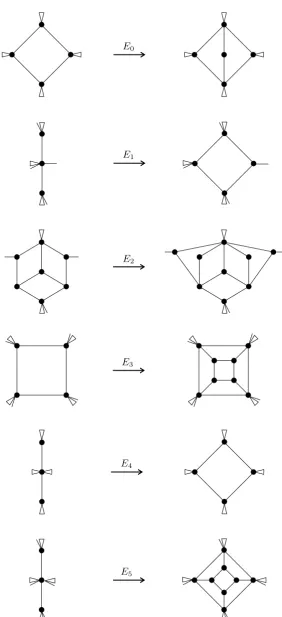
Quadrangulations

There are a basic set of expansion operations shown in Figure 3.2, small variations of which account for most generation theorems of classes of quadrangulations.

To get an overview, we start with the following main theorems in [17], in which the authors improved a number of existing theorems for generating simple quadrangulations.

Theorem 3.6(Brinkmann, Greenberg, Greenhill, McKay, Thomas, Wollan [17]).

Let the expansion operations be as labelled in Figure 3.2.

1. The class of all simple quadrangulations of the sphere can be generated from the square (C4) by the expansions E0 and E1.

2. The class of all simple quadrangulations of the sphere with minimum degree 3 can be generated from the pseudo-double wheels by E1 and E3.

3. The class of all 3-connected quadrangulations of the sphere can be generated from the pseudo-double wheels by E1 and E3.

4. The class of all 3-connected quadrangulations of the sphere in which all 4-cycles are facial is generated from the pseudo-double wheels by E1.

One reason that these classes of graphs are interesting is that they are pre-cisely the classes of radial graphs of the loopless 2-connected (but not necessarily simple) plane graphs, loopless 2-connected plane graphs without no facial digons nor vertices of degree 2, simple 2-vertex-connected and 3-edge-connected plane graphs, and simple 3-connected plane graphs respectively. In addition, their dual classes are the 4-edge-connected quartic plane graphs (not necessarily simple), simple 4-edge-connected quartic plane graphs, simple 3-connected quartic plane graphs, and (simple) 4-regular, 3-connected, 6-cyclically-connected plane graphs. These relationships are all discussed in [17].

(36)

E0

E1

E2

E3

E4

[image:36.595.133.416.91.710.2]

E5

(37)

For simple quadrangulations, a recursive structure was given by Negami and Nakamoto [66] and Batagelj [6] starting with the square and using the expansion E4. There are also several more recent approaches that are geared toward specific

theoretical applications. Bau, Matsumoto, Nakamoto and Zheng [8] define a recursive structure on this class which, in terms of reductions, uses E0-reductions

and some operations called hexagonal contractions which both have the property that the reduced graph is a minor of the original. Another approach by Fuchs and Gellert [36] also replaces E1-reductions by t-contractions, which are operations

that come up in the area of t-perfect graphs, and use this to characterise some classes of t-perfect graphs.

The simple quadrangulations with minimum degree 3 was first given a recur-sive structure by Nakamoto, using the same starting class but with operation E4 instead of E1. Again, the updated version is stronger in the sense that E1

is a more restrictive operation; there are linearly many E1 expansions possible

in a given simple quadrangulation, but E4 may permit a quadratic number of

expansions [17].

A generation theorem for 3-connected quadrangulations that are not necessar-ily simple was proposed (in the dual form) by Manca [58], however, an error was later found by Lehel [56] who corrected it by adding some expansion operations. Restricting to the subclass of simple graphs, Broersma, Duijvestijn and G¨obel [23] gave a generation theorem starting from the cube and using the operations E3,

E4 and a less restricted version of E2. More recently, Suzuki [82] gave another

alternative to Theorem 3.6(3) in which E3 is replaced by E5, which is known as

a cube contraction.

The classes of quadrangulations we have mentioned so far all consist of simple graphs. This is representative of results in literature with an exception being that K´apolnai, Domokos, and Szab´o [52] give a generation theorem for the class of arbitrary quadrangulations with no restrictions. We will discuss this in more detail when we define our own further classes of quadrangulations.

Pentangulations and beyond

(38)

theorems for k-edge-connected 5-regular planar graphs that are not necessarily simple for k up to 5 were also given by Ding, Kanno and Su [28], where the k = 0 case refers to arbitrary not necessarily connected graphs. This implies a generation theorems for pentangulations with girth k, so in particular the dual to the k = 3 case generates the simple pentangulations.

In Proposition 2.10, we showed that there are no simple planar k-regular graphs for k > 5. However, there is no such limit on simple k-angulations. The recursive generation of these classes has been studied by Jooyandeh [49].

3.1.2 Two related classes

For completeness, we will also record some generation theorems for related classes of graphs that are not necessarily planar.

General quartic graphs

Ding and Kanno [27] give generation theorems for quartic graphs that are not necessarily planar or simple. These classes are the arbitrary quartic graphs, con-nected quartic graphs, loopless quartic graphs, 2-edge-concon-nected loopless quartic graphs, 4-edge-connected loopless quartic graphs, simple quartic graphs, con-nected simple quartic graphs and 4-edge-concon-nected simple quartic graphs. Before this, a recursive structure for the simple quartic graphs had earlier been given by Bories, Jolivet and Fouquet [12].

k-angulations on surfaces

(39)

3.2. MORE CLASSES OF QUADRANGULATIONS 27

For quadrangulations, the most widely considered reduction operation is face contraction, which is operation E4 shown in Figure 3.2. It is proved in [67] that

an E4-irreducible quadrangulation of a closed surface Σ has at most 186(2 −

χ(Σ))−64 vertices, where χ(Σ) denotes the Euler characteristic. This implies that there are finitely many E4-irreducible quadrangulations (up to equivalence)

for any closed surface. So far, without repeating the spherical case which we have already seen, these have been determined completely for the projective plane [66], Klein bottle ([63], corrected in [80]), and torus [65]. In addition, for 3-connected quadrangulations, it is known thatE4-irreducibility is equivalent

toE3-irreducibility [62], and those that areE5-irreducible have been determined

for the projective plane [82].

3.2 More classes of quadrangulations

We now work toward bridging the gap between the results of Brinkmann et al. [17] on simple quadrangulations, K´apolnai, Domokos, and Szab´o [52] on the class of arbitrary multiquadrangulations, and those of Ding and Kanno [27] on quartic graphs that are not necessarily planar and not necessarily simple.

The classes of quadrangulations that we consider look, at first glance, a little unusual. We will see that one of them, namelyC3, is the class of 3-edge-connected

quadrangulations (Corollary 3.17). Secretly though, the underlying goal is to obtain recursive structures for a sequence of nice classes of quartic plane graphs that are similar to the results we have seen; they are defined by imposing certain conditions on connectedness and allowable non-simple structures. To phrase this in the more convenient land of quadrangulations, we need to characterise the duals of the classes we wish to generate.

(40)

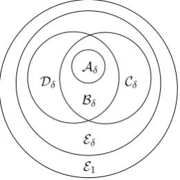
Curtains Sunnies e-Sunnies

Figure 3.3: Forbidden families in some classes of quadrangulations.

Letδ denote a lower bound on the minimum degree. A standard application of Euler’s formula shows that every quadrangulation has average degree strictly less than 4 and hence has minimum degree at most 3. This leads to the following classes of quadrangulations, where δ= 2 or 3:

Aδ Simple quadrangulations of the sphere.

Bδ Quadrangulations of the sphere excluding curtains and sunnies.

Cδ Quadrangulations of the sphere excluding curtains and e-sunnies.

Dδ Quadrangulations of the sphere excluding sunnies.

Eδ Arbitrary quadrangulations of the sphere with given minimum degree.

E1 Arbitrary quadrangulations of the sphere.

E1

Eδ

Dδ Cδ

[image:40.595.212.343.453.584.2]

Bδ Aδ

Figure 3.4: Inclusions of our classes of quadrangulations, fixingδ as 1 or 2.

(41)

Here’s a handy list of the classes of quartic plane graphs dual to each of the classes defined above. A cluster of facial digons refers to the structures shown in Figure 3.5. We defer the proofs until Section 3.2.2.

A∗

3 Simple 4-edge-connected quartic plane graphs. (Theorem 3.14)

A∗

2 4-edge-connected quartic plane graphs. (Theorem 3.14)

B∗

3 Simple 2-connected quartic plane graphs. (Theorem 3.15)

B∗

2 2-connected quartic plane graphs that are simple except for those clusters

of facial digons shown in Figure 3.5. (Theorem 3.15) C∗

3 Simple quartic plane graphs. (Theorem 3.16)

C∗

2 Quartic plane graphs that are simple except for clusters of facial digons.

(Theorem 3.16) D∗

3 2-connected quartic plane graphs without facial digons or loops.

(Theo-rem 3.18) D∗

2 Loopless 2-connected quartic plane graphs. (Theorem 3.18)

E∗

3 Quartic plane graphs without facial digons or loops. (Theorem 3.19)

E∗

2 Loopless quartic plane graphs. (Theorem 3.19)

E∗

1 Arbitrary quartic plane graphs. (Theorem 3.19)

3.2.1 Generation theorems

The operations used to generate a particular class of quadrangulations from an earlier class are known as expansions. Applying an expansion will not always result in a strictly larger quadrangulation, but it will introduce some more general structure. We will use the five expansion operations shown in Figure 3.6. To make the displayed expansion operations precise, we detail their associated reductions as follows.

• Suppose we have a 6-cycle v1 e1 —v2 e2 —v3 e3 —v4 e4 —v5 e5 —v6 e6

—v1 together with a

digonv1 c1

—v4 c2

—v1 such thatv1 e1 —v2 e2 —v3 e3 —v4 c1

—v1 andv1 c1 —v4 e4 —v5 e5 —v6 e6

—v1 are

facial cycles. A P-reduction consists of deleting the c2 and inserting an

edge between v3 and v6. By planarity, there is only one way to do this up

to equivalence so the cyclic order at each vertex is completely determined.

• A P2-reduction is the same as a P-reduction except that it can only be

(42)

• A P1-reduction is also the same as a P-reduction except that it can only be

applied when e2 is simple, there exists an edge e05 parallel to e5 which does

not share a face with c2, and the region bounded by v1 e6 —v6 e0 5 —v5 e4 —v4 c1

—v1 is

non-facial.

• A Q2-reduction may be applied when there is a face bounded by a circuit

of the form v1 e1 —v2 e2 —v1 e3 —v3 e4

—v1, with the condition thatv1 andv3 are both

incident to edges inside the region bounded by the digon v1 e4

—v3 e3

—v1 that

does not contain v2. The reduction then consists of identifying v2 and v3

to form a new vertex v₂0, as well as identifying e1 with e4 and e2 with e3 to

form new edges e0₁ and e0₂ that both have as endverticesv1 and v20.

• A Q1-reduction may be applied when there is a face bounded by a walk of

the form v1 e1 —v2 e2 —v1 e3 —v3 e3

—v1, and consists of identifying v2 and v3 to form

a new vertex v₂0, as well as identifying all three edges e1, e2 and e3 into a

single edge e0₁ with endvertices v1 and v20.

We can already generate Aδ (Theorem 3.6(1) and (2)), so we will use these

are starting classes to find recursive structures for each of the later classes in sequence. K´apolnai, Domokos, and Szab´o [52] showed that E1 can be generated

from P2 using the operations E0, E1 and Q1. Our generation theorem for this

class is not as efficient as theirs since we use more operations. Nonetheless, the scenic route that we take allows us to obtain generation theorems for the other eight new subclasses of quadrangulations.

For each of the following generation theorems, the idea is to show that any graph in the target class is reducible via the specified operation(s), and that the reduced graph in each case is still in the class. This would then imply that the required sequence of graphs can be found by recursively applying reductions. The following face lemma will help us to do this.

Lemma 3.7. All faces of a quadrangulation of the sphere take one of the types A, B, C or D shown in Figure 3.7.

Proof. Each face is bounded by some 4-cycle v1 e1 —v2 e2 —v3 e3 —v4 e4

—v1. To enumerate

the possible faces, we need to consider all possible ways that some of these edges and vertices might be the same. Firstly, if all edges and vertices are distinct then we have face type A. Otherwise we must have at least two vertices be the same. Since there are no loops, it is only possible thatv1 =v3orv2 =v4. Moreover, it is

(43)

P _v

1

e1 v2

e2

v3 _e₃

v4 e4 v5 e5 v6 e6 c2 c1 v1

e1 v2

e2

v3 _e 3 v4 e4 v5 e5 v6 e6 c2 c1

P2 _v

1

e1 v2

e2

v3 _e₃

v4 e4 v5 e5 v6 e6 c2 c1 v1

e1 v2

e2

v3 _e 3 v4 e4 v5 e5 v6 e6 c2 c1

P1 _v₁

e1 v2

e2

v3 _e₃

v4

e4

v5

e5

e0₅ v6

e6

c2

c1

v1

e1 v2

e2

v3 _e 3

v4

e4

v5

e5

e0₅ v6

e6

c2

c1

Q2 v1 v2

v3

e1

e2

e3

e4

v1 v20

e0₁

e0₂

Q1 v1 v2

v3

e1

e2

e3

v1 v02

[image:43.595.159.480.147.639.2]

e01

(44)

loss of generality, supposev2 =v4. If all edges are then distinct, we obtain a face

of type B, shown in the figure as both a bounded region or as an outside face. Otherwise, the only possible edge identifications are e2 =e3 ore1 =e4, the other

possibilities being excluded since they would create loops. When exactly one of these is true we have a face of type C, again drawn as both an inside and outside face in the figure, and when both hold we get a face of type D.

Type A Type B Type C Type D

Figure 3.7: All possible faces of length four.

We are now ready to state our first generation theorem in the sequence.

Theorem 3.8. The class Bδ (δ = 2,3) of all quadrangulations of the sphere

excluding curtains and sunnies is generated fromAδ by the operations P2 andP1.

Proof. Let G be a graph in Bδ − Aδ. We first show that every face in G is

bounded by a simple cycle. This follows from Lemma 3.7 since of the possible faces in Figure 3.7, types C and D cannot occur asδ≥2 and any graph containing a type B face is in the family of sunnies. This leaves only face type A, which is the one we wanted. Now since G 6∈ Aδ, it must be non-simple. Moreover, since

it is bipartite and hence has no loops, this means that it must contain parallel edges.

Fix a planar embedding of G and pick a pair of innermost parallel edges c1 and c2 with endvertices v1 and v4; by innermost we mean the union of the

subgraph contained inside the digonc1c2 together with the digon itself is simple.

Consider the simple cycles bounding the two faces adjacent to c2. Applying the

Jordan curve theorem to the digon c1c2, we see that the vertex sets of these two

simple cycles intersect only in v1 and v3, and their disjoint union is a 6-cycle

v1 e1

—v2 e2

—v3 e3

—v4 e4

—v5 e5

—v6 e6

—v1. Let’s suppose these are labelled so that v2 and v3

are inside c1c2.

Now consider the edges e2 and e5. By choice of c1 and c2, we know that e2

(45)

On the other hand, if e5 is not simple then we claim that a P1-reduction can be

applied. Say e5 is parallel toe05, labelled so thate5 and c2 share a face. The only

possible obstruction to the reduction is if v1 e6 —v6 e0 5 —v5 e4 —v4 c1

—v1 is a facial cycle.

However, we observe that if this is the case then the graph is a curtain as shown in Figure 3.8, which cannot occur.

v1 e1 v2 e2 v3 e3 v4 e4 v5 v6

e6 e5

e0₅ c2

[image:45.595.252.389.207.344.2]

c1

Figure 3.8: The solid lines form a forbidden curtain.

It remains to show that after applying either of these reductions, the resulting graph is still in Bδ. Since both operations remove a parallel edge and cannot

create a new one due to the ordering of c1 at v1 and v4, it is not possible for

either reduction to produce a graph in the family of curtains or sunnies. For the degree condition, it is enough to note that d(v1) and d(v4) are at least 4 prior

to the reduction, and so are at least 3 afterward. No other vertices decrease in degree.

Theorem 3.9. The class Dδ of all quadrangulations of the sphere excluding

sun-nies is generated from Bδ by operation P.

Proof. Take any G in Dδ − Bδ. The same argument as before shows that every

face in G is bounded by a simple cycle. From the definitions of the classes, G must be a curtain, so in particular let v1

c1

—v4 c2

—v1 be one of the defining digons.

We can now follow the previous proof, but where we differentiated between the two operations previously, we find that in all cases the graph isP-reducible. The verification that degree bounds are preserved and the reduced graph is not in the family of sunnies still holds.

Theorem 3.10. The class Cδ of all quadrangulations of the sphere excluding

(46)

Proof. If G is in Cδ − Bδ, then it must contain sunnies that are not e-sunnies.

To start with, we will just use the existence of type B faces. Pick any type B face, say bounded by the circuit v1

e1 —v2 e2 —v1 e3 —v3 e4

—v1, and fix an embedding of G

so that this face is not the outer face. Now consider the digon v1 e4

—v3 e3

—v1. This

is necessarily non-facial, so let H denote the subgraph of G contained inside this digon. Suppose H is adjacent to only one of v1 or v3. If it is adjacent to v3,

then there must be a vertex v4 and parallel edges e5 and e6 between v3 and v4 in

order to ensure the face inside the digon adjacent to e3 and e4 has length four.

Furthermore, e5 and e6 must be distinct, otherwise v4 would have degree 1. But

G is not in the family of e-sunnies, so H must be adjacent to v1 only. At this

point we have d(v3) = 2, so if δ = 3 then this situation is impossible. Thus, H

must be adjacent to both v1 and v3 and we may apply an Q2-reduction. Note

that since e1e2 has length 2, the region outside this digon is non-facial since Gis

a quadrangulation.

Forδ = 2, we can still show that there is exists a type B face for which H is adjacent to both v1 and v3. Under the previous labelling, if haveH adjacent to

onlyv1 then as before there is a face inside the digon v1 e3

—v3 e4

—v1 that is adjacent

to both e3 and e4. In order for this to be bounded by a walk of length 4, we must

be now have a vertex v4 and distinct parallel edges e5 and e6 between v1 and v4

so that v1 e4 —v3 e3 —v1 e5 —v4 e6

—v1 is a face of G. This is gives another type B face, as

can be seen in Figure 3.9, which we shall declare to be inside our original one. We now have the notion of an innermost type B face. Choosing such a face and again using the same labelling, the property that it is innermost guarantees that H must be adjacent to bothv1 andv3 so as before we find thatGisQ2-reducible.

v1

v4 v3

[image:46.595.204.352.532.631.2]

v2 e1 e3 e4 e2 e6 e5

Figure 3.9: An inner type B face (shaded) inside a larger one.

(47)

with either e1e2 or e3e4 allow us to draw G as a member of the curtain family

which is a contradiction. Similarly, the reduced graph cannot be in the family of e-sunnies. Also, before the reduction d(v1) ≥ 5 so the degree is at least 3

afterward, and no other vertices that survive the reduction have lower degrees. Therefore,Q2(G)∈ Cδ.

Theorem 3.11. The class Eδ of all quadrangulations of the sphere with given δ

is generated from Dδ by operation Q2.

Proof. We use similar reasoning as in the proof of Theorem 3.10. IfG∈ Eδ− Dδ,

then it must be in the family of sunnies, and consequently has a type B face. Using the notation and argument in theδ = 2 case of the previous proof, one can find an innermost type B face on which to apply a Q2-reduction. The argument

that the degree bounds are preserved also carries over.

Theorem 3.12. Except for the path of three vertices, the class E1 of arbitrary

quadrangulations of the sphere is generated from E2 by operation Q1.

Proof. Let G be a graph in E1 − E2, meaning it must have a degree 1 vertex.

By Lemma 3.7, any face containing a vertex of degree 1 is of type C or type D. The latter is unique to the case where G is a path with three vertices, so in all other graphs we must have a type C face. This is exactly the form needed to apply aQ1-reduction, and doing so cannot produce isolated vertices so the degree

condition is met.

3.2.2 Characterising the duals

The proofs of the dual relationships we listed earlier are relatively straightforward once we attain some fluency in translating between various properties of a graph and the corresponding properties or structures of its dual. We have already seen cut-cycle duality (Lemma 2.23), which gives one result of this type. The following lemma spells out the correspondence between key structures that appear in our classes and their duals.

Lemma 3.13 (Dual structures). SupposeGis a quadrangulation, or equivalently that G∗ is quartic.

(a) If G is simple and G∗ is 4-edge-connected, then G has a vertex of degree 2 if and only if G∗ has parallel edges.

(48)

(c) Gis in the family of curtains or e-sunnies if and only if G∗ has a non-facial digon.

(d) If G∗ is 2-vertex-connected, then G is in the family of curtains if and only if G∗ has a non-facial digon.

(e) G has a degree 2 vertex if and only if G∗ has a facial digon.

(f ) G has a degree 1 vertex if and only if G∗ has a loop.

Proof. (a) By examining the picture on the right of Figure 3.10, one observes that if Ghas a vertex of degree 2 (this is a 2-edge cut), then the dual, drawn with unfilled vertices and red edges, must have a digon so this direction is straightfor-ward. Suppose instead that we start with a digon in G∗. If the region inside the digon were a face, then the vertex corresponding to this face in the dual would have degree two, so we would be done in this case. Otherwise, there is some part of the graphG∗ contained in the shaded region as shown in the left of Figure 3.10. Since G∗ is 4-edge-connected, there must be four edges connecting this part of the graph to the digon, and the configuration drawn with two edges between the shaded region and each vertex of the digon is the only possibility. However, we have now accounted for all four edges adjacent to the vertices in the digon, and since G∗ is connected, this means that all of G∗ must actually be within the shaded region. In particular, the outside region of the digon is a face, and hence corresponds to a vertex of degree 2 in G.

Figure 3.10: Degree two vertices in A3 are dual to facial digons in Q.

(49)

see from the same figure that G has a 1-cut consisting of the vertex dual to the outer face.

Figure 3.11: Sunnies are dual to 1-cuts

(c) Suppose there is a non-facial digon in G∗. Since it is quartic, there are four possible configurations of edges at the two vertices in the digon, and these are shown in Figure 3.12. From the left, the 00-digon is facial so we will not consider it. The 01-configuration has an unbalanced 1-vertex-cut which violates our characterisation in Section 2.3.1. The last two configurations are possible.

00 01 02 11

Figure 3.12: Possible configurations of digons in a quartic graph.

[image:49.595.254.383.148.233.2]

If the 02-configuration is present, the graph has the structure of the red graph on the right of Figure 3.13. In the dual G, drawn in solid black, observe that in each region bounded by the digon the two vertices of G shown must exist and be distinct since G being loopless implies that G∗ cannot have any 1-edge-cuts. Thus,G is in the family of e-sunnies.

(50)

Similarly, if the 11-configuration is present thenG∗ has the structure of the red graph on the right of Figure 3.14. Again, the shaded regions must be connected subgraphs ofG∗ to avoid 1-edge-cuts, and we see that the dualGis in the family of curtains.

Figure 3.14: Curtains are dual to 11-digons.

Conversely, ifG is in the family of e-sunnies or curtains then the pictures on the left hand side of Figure 3.13 and Figure 3.14 respectively show that we get either a 11- or 02-digon in G∗, both of which are non-facial.

(d) If G is in the family of curtains then we have already seen in (c) that G∗ has a digon, and moreover by inspecting Figure 3.14 we observe that it is non-facial. The converse can also be shown easily following the argument from part (c). Returning to the digon configurations from Figure 3.12, we may still ignore the first two possibilities. The assumption that G∗ is 2-connected now also excludes the 02-configuration as both vertices in the digon are 1-cuts. Thus, only the fourth configuration can occur, and we have already shown that this corresponds Gbeing in the family of curtains.

(e) This is a basic observation.

(f) Certainly ifGhas a degree 1 vertex, then the dual has a loop. Conversely, if G∗ has a loop then G must have a bridge, since removing the edge dual to the loop will disconnect the graph. We observe that any bridge in a quadrangulation is adjacent to a vertex of degree 1 since there are no loops and the bridge must occur twice in the facial circuit that contains it.

(51)

Theorem 3.14. A∗

3 is the class of simple 4-edge-connected quartic plane graphs,

and A∗

2 is the class of 4-edge-connected quartic plane graphs.

Proof. Let Q4E denote the class of 4-edge-connected quartic plane graphs, and QS4E the class of simple 4-edge-connected quartic plane graphs. We begin with the second statement. It is elementary that quadrangulations are dual to quartic plane graphs, so we only need to check the remaining conditions. Let G be any graph in A2. Observe that G has no loops or digons since it is simple, and no

3-cycles since it is bipartite so by cut-cycle duality it follows that G∗ is 4-edge-connected. Thus, A∗

2 ⊆Q4E. Conversely, if H is some graph in Q4E, then H is

4-edge-connected and cut-cycle duality immediately implies thatH∗ has no loops or parallel edges. Any graph is isomorphic to its double dual, so this shows that Q4E ⊆ A∗

2 which now gives the second statement.

Since A∗

3 ⊂ A

∗

2, we already know that the dual of any graph G ∈ A3 is a

4-edge-connected plane quartic graph. To prove that A∗

3 = QS4E now, we just

need to show that a graph in Q4E is simple if and only if its dual has minimum degree three. Since simple quadrangulations are bridgeless and hence their duals are loopless, then this is equivalent to showing that a graph in A∗

2 has a vertex

of degree two if and only if its dual has parallel edges which is the content of Lemma 3.13(a).

Theorem 3.15. B∗

3 is the class of simple 2-connected quartic plane graphs, and

B∗

2 is the class of 2-connected quartic plane graphs that are simple except for facial

digons.

Proof. Let QS2 be the class of simple 2-connected quartic planar graphs, and QS2+_{denote the class of 2-connected quartic planar graphs that are simple except}

for facial digons. We will start by showing the first part of the statement. Suppose G ∈ B3. It is straightforward to establish that G∗ is a loopless quartic plane

graph. By Lemma 3.13(b), since sunnies are forbidden from B3 it follows that

G∗ must be 2-connected. As G has no curtains, G∗ has no non-facial digons by Lemma 3.13(d), and asδ = 3 it follows from Lemma 3.13(e) thatG∗ has no facial digons either. That is, G∗ has no parallel edges and hence is simple. Therefore, B∗

3 ⊆QS2. Starting instead with an arbitrary graph H =G

∗ _∈_{QS2, then} _G_{is a}