Dead-beat control for polynomial systems

(1)

Dead-Beat Control for Polynomial

Systems

..

Dragan N

esic

Bachelor of Engineering

August 1996

A thesis submitted for the degree of Doctor of Philosophy

of the Australian National University

Department of Systems Engineering

Research School of Information Science and Engineering

(2)

To

my family

Ksenija and Nina

and my parents

Dragica and Dusan

(3)

Statement of originality

The contents of this thesis are the results of the original research unless otherwise stated and have not been submitted for a higher degree at any other university or institution. The material described in this thesis has been obtained under the supervision of Prof. I. M. Y. Mareels. Some results have been obtained in cooperation with Prof. G. Bastin and Dr. R. Mahony. However, the majority of work, approximately 90 %, is my own.

The following journal papers follow from the material presented in the thesis:

1. D. Nesic, "A note on dead-beat controllability of generalised Hammerstein systems", to appear in Systems and Control Letters.

2. D. Nesic and I. M. Y. Mareels, "Output dead beat control for a class of planar polynomial systems", submitted in 1995, first revision completed

3. D. Nesic and I. M. Y. Mareels, "Dead beat controllability of polynomial systems: symbolic computation approaches", submitted in 1995, first revision completed.

4. D. Ne sic and I. M. Y. Maree ls, "Dead beat control of polynomial scalar systems", in revision. 5. D. Nesic and I. M. Y. Mareels, "Dead beat control of simple Hammerstein systems", in

rev1s1on.

6. D. Nesic and I. M. Y. Mareels, "State dead beat controllability of structured polynomial systems", in preparation.

7. D. Nesic and I. M. Y. Mareels, "Stability of implicit and explicit polynomial systems: symbolic computation approaches", in preparation.

A number of conference papers follows from the results presented in the thesis. Some of the material in these papers overlaps with that covered in the journal papers.

1. D. Nesic, I. _{M. Y. Mareels, R. Mahony and G. Bastin, " 11-step controllability of scalar} polynomial systems", Proc. 3rd ECC, Rome, Italy, pp. 277-282, 1995.

2. D. Nesic, I. M. Y. Mareels, G. Bastin and R. Mahony, "Necessary and sufficient conditions for output dead beat controllability for a class of polynomial systems", Proc. CDC, New Orleans, pp. 7-13, 1995.

(4)

3. D. Nesic and I. M. Y. Mareels, "Invariant sets and output dead beat controllability for odd polynomial systems: the Grabner basis method", Proc. 13th IFAC World Congress, San Francisco, vol. E, pp. 221-226, 1996.

4. D. Nesic, I. M. Y. Mareels, G. Bastin and R. Mahony, "Stability of implicitly defined polynomial dynamics: the scalar case", presented at MTNS, St. Louis, 1996.

5. D. Nesic and I. M. Y. Mareels, "Deciding dead beat controllability using QEPCAD", presented at MTNS, St. Louis, 1996.

6. D. Nesic and I. M. Y. Mareels, "Minimum time dead beat control of simple Hammerstein systems", presented at MTNS, St. Louis, 1996.

7. D. Nesic and I. M. Y. Mareels, "The definition of minimum phase discrete-time nonlinear systems revisited", to appear in Proc. ICARV '96, Singapore.

8. D. Nesic and I. M. Y. Mareels, "Scalar polynomial systems, triangular structures and dead-beat controllability", submitted in 1996.

9. D. Nesic and I. M. Y. Mareels, "Stability of high order implicit polynomial dynamics", submitted in 1996.

10. D. Nesic and I.

M. Y.

Mareels, "An output dead beat controllability test for a class of odd polynomial systems", submitted in 1996.

11. D. Nesic and I. M. Y. Mareels, "On some triangular structures and the state dead beat problem for polynomial systems", submitted in 1996.

~[v;

~v~~c

Department of Systems Engineering

Research School of Information Science and Engineering The Australian National University

(5)

Acknowledgements

I would like to take this opportunity to thank my supervisor Prof. Iven M. Y. Mareels for his encouragement, support and for being such a nice person to work with. Iven has shown a remarkable patience with me in situations when I needed it most. Because of the war in my country, I undergone several personal crises in the last two years. During this time, my supervisors' help and support was invaluable in keeping my interest in research despite the national tragedy which happened in Yugoslavia. Iven's enthusiasm and excitement about new research ideas, his open mind to new and sometimes controversial concepts and his high standards in research made the time spent with him professionally very inspiring and fulfilling. His efforts to introduce me and my ideas to a number of people in the control community resulted in my visits to several conferences, universities and organisations, which was a great experience. Also, thanks to Iven I am one of the lucky students who got a chance to give several lectures on the subject of Digitally Controlled Systems. Having said all of this, I would like to thank Iven once again for exposing me to virtually every possible aspect of research life, from which I benefited a lot. Finally, I must admit that, apart from my research, the greatest challenge in the last two years was to beat Iven in table-tennis, which I managed just a few times.

I have cooperated with Prof. G. Bastin, Prof. H. Nijmeijer and Dr. R. Mahony and I would like to thank them for their patience and support. In particular I would like to convey my gratitude to Prof. G. Bastin whose support made possible my visit to Catholic University in Louvaine la Neuve. I express my sincerest gratitude to Prof. G. Bastin, Dr. R. Mahony and Dr. P. Bartlett for carefully reading parts of this manuscript.

I am indebted to Prof. G. E. Collins for his advice on QEPCAD, as well as for his effort in solving some problems that I had sent to him. The CRC for Robust and Adaptive Systems funded most of my visits to universities and attendance to workshops and conferences during my studies and I am grateful for that.

I would also like to thank my wife Nina and daughter Ksenija for their never ending love, support and understanding, without which this work would be much more difficult. The support and encouragement that I got from my family, relatives and friends was also very important to me and I thank them for this.

Last but not least, I would like to thank to all the students and staff for making such a stimulating and friendly atmosphere at the Department of Systems Engineering.

(6)

(7)

II·

ABSTRACT

This thesis contributes to a better understanding of state and output dead-beat control problems and stability of zero output constrained dynamics for the class of discrete-time polynomial systems. Dead-beat controllability is one of the fundamental notions in control theory since it establishes the existence of control laws which can achieve a desired operating regime in finite time. The class of polynomial systems that we consider is very broad. Indeed, under very mild assumptions any nonlinear input-output map can be realised by a polynomial model.

Symbolic computation methods are exploited to tackle the dead-beat control problems. An algorithm for the design of minimum-time dead-beat controllers follows from our approach. In principle, the proposed method can deal with multi-input multi-output systems and bounds on controls and states can be included in a straightforward manner. The price we pay is the large computational cost, which prevent us from using this method in general.

To reduce the computational requirements for our controllability tests and design method-ologies a number of simpler classes of polynomial systems are considered. Mathematical tools, such as algebraic geometry, real algebraic geometry, symbolic computation and convex analysis,

are exploited. In this way, a number of analytic results are obtained with which we obtain com-putationally feasible controllability tests and design methodologies, as well as gain some more geometric insight.

Stability of zero output constrained dynamics and the related minimum phase property play an important role _in output dead-beat control. The definitions found in the literature are not general enough to incorporate all behaviours that may occur in the context of polynomial systems. We revisit the definition of a minimum phase system and propose symbolic computation means to test different minimum phase properties for polynomial systems. Our results can be used for testing stability and stabilisability either by definition or by constructing Lyapunov functions.

(8)

(9)

IR,N,2,Q,C

]:Rn

k[x1,.,,,xn]

I

vlJ

(/1, .. ·,

fn)

V(f1, ... , f2) l(V)

AC B, Ac B

AnB

AUE

A-B

A V

:l

V fig

av

vc

0 'D card'D ~ S(x), S(x)

rankA

AT

dimV

im(f)

Notation:

-The sets of real, natural, integer, rational and complex numbers. The set of all n-tuples (vectors) of real numbers.

Ring of polynomials with coefficients in the field k. Ideal.

Radical ideal.

Ideal generated by polynomials

/1,

... ,

fn•

Variety of the polynomials !1,

... ,

f

n.

Ideal of a variety V.

A

is a subset of B,

A

is a proper subset of B. Intersection of sets A and B.

Union of sets

A

and

B.

The set { x : x E

A, x

(j.

B}.

Conjunction operator (and). Disjunction operator (or). Existential quantifier. Universal quantifier.

f, g

E IR[x1, ... , Xn] and g divides

J.

Boundary of the set 'D C IR n.

Complement of the set 'D C IR n with respect to IR n. Interior of the set 'D C IR n.

Cardinal number of the set 'D.

~ Defining formulas for semi-algebraic sets Sand S The rank of the matrix

A.

Transpose of the matrix

A.

The dimension of a variety V The image of the function

J.

Gbasis [j 1, ... ,

f

nl

The reduced Gro bner basis for polynomials

J

1 , ... ,

J

n. X

>-

y x is ranked higher than y using an ordering.

(10)

ARMAX

CAD

I-0

MI

MIMO

NARMAX

PID

PI

QE

QEPCAD

SISO

Abbreviations:

Auto-Regressive Moving Average with eXogenous input.

Cylindrical Algebraic Decomposition

Input-Output

Multi-Input

Multi-Input Multi-Output

Nonlinear Auto-Regressive Moving Average with eXogenous input.

Proportional Integral Differential

Proportional Integral

Quantifier Elimination

Quantifier Elimination by Partial Cylindrical Algebraic Decomposition

(11)

I

Dead-Beat Controllability and Control of Polynomial Systems

1

Introduction

1.1 Nonlinear Discrete-Time Systems . . . . 1.2 Motivation . . . .

1.2.1 Polynomial Systems . . . .

1.2.2 Dead-Beat Controllability and Control . . . . 1.2.3 Minimum Phase Polynomial Systems . . . .

1.2.4 On the Tools that are Used . . . .

1.3 Overview of the Literature . . . . 1.3.1 Linear Dead-Beat Control . . . . 1.3.2 Nonlinear Dead-Beat Control . . .

.

. . .

.

1.3.3 Implementations: pro et contra

.

. .

. . .

.

. .

.

. .

.

1.4 Outline of the Thesis . . .

.

. .

.

2

Preliminaries

2.1 Notation and Definitions . . .

2.2 General Assumptions

.

_.

.

_{. .}

.

_.

. .

_{. . . .}

_.

. . .

.

_.

.

_.

.

_.

2.3 A Prelude

. . .

.

_.

. . .

. .

.

. .

.

. . .

.

. .

.

. . .

2.3.1 _{Linear Dead-Beat Control . . . .}

2.3.2 _{Nonlinear Dead-Beat Control . . . .}

3 Deciding Dead-Beat Controllability Using QEPCAD

3.1 Introduction . . .

3.2 Class of Systems . . .

3.3 A Short Introduction to QEPCAD

Xl

1

3

6

10

12

13

15

18

23

24

31

34

36

38

41

42

(12)

3.4 State Dead-Beat Control . . . .

3.4.1 Computation of Sets

sk

and

sk

3.4.2 State Dead-Beat Controllability Tests

3.5 Output Dead-Beat Control . . . .

3.5.1 Computation of Sets

Tj

and

Sf

3.5.2 Output Dead-Beat Controllability Test .

3.6 Examples .

3.7 Conclusion .

4 Odd Polynomial Systems

4.1 Introduction . . . . .

4.2 Definition of the System . . . .

4.3 Invariant Sets and Output Dead-Beat Controllability ..

4.4 Examples . . . .

4.5 Case Study 1: Column-Type Grain Dryer

4.6 Conclusion . . . .

5 Scalar Polynomial Systems

5.1 Introduction . . . .

5.2 Notation and Definitions

5.3 A Necessary Condition for Dead-Beat Controllability .

5.4 Odd Systems . . . .

5.5 Even Systems . . . .

5.5.1 Case 1 . . . .

5.5.2 Case 2

5.5.3 Case 3

5.6 Main Result . .

5.7 An Algebraic Test for Dead-Beat Controllability . .

5.8 Comparison with Some Known Results

5. 9 Local Dead-Beat Stabilisability . . . .

5.10 Local Dead-Beat Stabilisability with a Bounded Control Signal

5.11 Examples . . . .

5.12 Case Study 2: a Heat Exchanger . .

44 45 48 55 55 57 59 64

65

65 66 67 74 78 81

83

84 85 87 90

92

93 93 94 99

. . 102

. 105

. 106

. 107

(13)

.

. . .

.

. . . .

.

... .

. 112

6 A Class of Odd Polynomial Systems

115 .

.

. . . .

.

. .

.

. . . 115

6.2 Pr e lim" . 1nar1es . . . . . . . . 116

6.3 Output Dead-Beat Controllability . . . . . 119

6.4 Output Dead-Beat Controllability Tests

....

. . . . 123

6.5 Examples . . . . . . . . . 127

6.6 Conclusions . . . .

.

. .

.

. . .

. . . .

. . .

.

. .

.

. . . 134

7 Simple Hammerstein Systems

135

7.1

Introduction . . . .

.

. . . .

. . . 135

7.2 Notation and Definitions . . . 137

7.3 Dead-Beat Controllability . . . . . . 138

7.4 State Dead-Beat Controllers . . . . 140

7.4.1 Scalar Case

. . .

.

. .

.

. . .

.

. . . 140

7.4.2 Controller 1: Second Order Systems . . . 140

7.4.3 Controller 2 . . . . . . 144

7.4.4 Controller 3: General Case . . . . . . . 148

7.5 An Output Dead-Beat Controller . . . 151

7.6 Examples . . . . . . . . . . . . . . . 153

7.7

Conclusion . . . .

.

. . . 159

8 Generalised Hammerstein Systems

₁₆₁

8.1 Introduction . . . . . 161

8.2 Main Result

.

. . .

. .

.

. .

.

. . . .

.. 162

8.3 Examples . . . 167

8.4 Conclusion . . .

. . . .

.

. .

. . . ..

. . . 170

9 Structured Polynomial Systems 9.1 Introduction

171

. . 171

.. 172

175 .. 178 9.2 Class 1 . . .

9.2.1 Minimum-Time Dead-Beat Controller . .

9.2.2 Class 1: Examples . . . .

(14)

9.3 Class 2 . . . .

9.3.1 Class 2: Examples .

9.4 Class 3 . . . .

9 .4.1 Strict Feedback Polynomial Systems

9.4.2 Class 3: Examples .

10 A Simulation Study: Biochemical Reactor

10.2 The Simulation Study

II Minimum Phase Polynomial Systems and Stable Zero Dynamics

11 Minimum Phase Polynomial Systems

11.1 Introduction

11.2 Motivation .

11.3 A QEPCAD Based Minimum Phase Tests .

11.3.1 Preliminaries .

11.3.2 Main Results .

11.4 Scalar Implicit Dynamics

11.4.1 An Algebraic Set-Minimum Phase Test

11.4.2 Examples . . . .

11.4.3 _{Output Dead-Beat Control Law With Stable Zero Dynamics}

11.4.4 Case Study 3: a Fan and Radiator System .

12 Conclusions and Further Research

12.1 Conclusions . . .

12.2 Further Research .

. . . . . 180

. 183

. . . 185

. 187

. 190

. 193

195

.. 195

.. 196 .. 199

201

203

. . 203 . . 204 . 210

.. 211

. 217 . . 225 . 230

. 234

. 237

. . 239

. 241

245

. . 245 . 250

12.2.1 Conditions for Dead-Beat Controllability/Stabilisability for Polynomial

(15)

12.2.5 Dead-Beat Controllability of Non-Polynomial Systems 12.2.6 Other Control Laws . . . .

ID Appendices

A Polynomial Models

A.1 Applications of Polynomial Models

A.2 Classes of Polynomial Models Used in the Literature

B Mathematical Background Material

B.1 Algebraic Geometry

.. 255 . 255

257

259

. 259 . . . 262

264

. . 264 B.2 Grabner Bases . . . . 265 B.2.1 Complexity of Grabner Basis Constructions . . . 269 B.3 Semi-Algebraic Geometry . . . . 270

B.3.1 Cylindrical Algebraic Decomposition (CAD) and Quantifier Elimination

(QE) . . . . 275 B.3.2 Computational Complexity of the QEPCAD Algorithm .

B.3.3 An illustrative Example . . . .

xv

. . 277 . . 278

(16)

Part I

Dead-Beat Controllability and Control

of Polynomial Systems

(17)

(18)

Chapter 1 Introduction

The purpose of this chapter is in the first instance to emphasize the importance of the theory of discrete-time nonlinear systems. The main topic of the thesis, dead-beat control for polynomial discrete-time systems, is introduced and motivated. An overview of the existing literature dealing with dead-beat controllability is provided. The chapter is concluded with the outline of the thesis, highlighting the main contributions.

1.1 Nonlinear Discrete-Time Systems

In the last 40 years the control community has witnessed tremendous advances in computer tech-nology which have had a great impact on the control systems theory and applications. Advances in hardware provided the control engineer with more powerful, reliable, faster and above all cheaper computers that could be implemented as process controllers. A good historical account of the genesis of digitally controlled systems is given in [6]. Today, almost all controllers are computer implemented. Consequently, the theory, which is used to design digital controllers and explain the phenomena that occur, is of utmost importance.

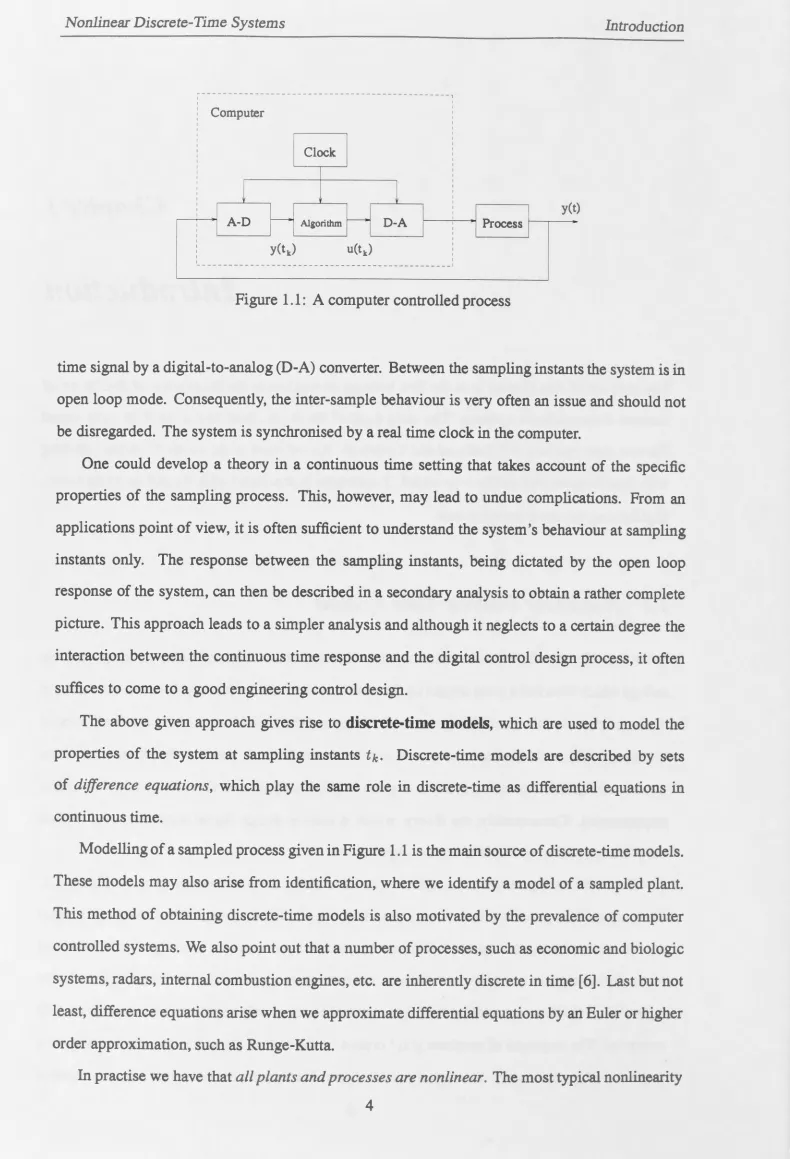
The usual configuration of computer controlled closed loop systems is given in Figure 1.1. The output of the process y ( t) _{is a continuous time signal. The measurements of the output signal} are fed into an analog-to-digital (A-D) converter, where the continuous time signal is transformed into a digital signal - a sequence of measurements at sampling times tk.

If a measurement device

is itself digital, the measurements are taken at sampling times only and there is no need for an A-D converter. The sequence of numbers y(tk) is used by the control algorithm in order to compute a sequence of controls u(tk) - _{the digital control signal. The sequence is converted into a continuous}

(19)

~---, Computer

l

I I ~ A-D I I I I y(t1J I I I Clock

Algorithm ,---.

[image:19.845.44.834.44.1203.2]

U(tk)

l

D-A I I I I I I I I I I I I I I I ---1 Process

Figure 1.1: A computer controlled process

y(t )

time signal by a digital-to-analog (D-A) converter. Between the sampling instants the system is in open loop mode. Consequently, the inter-sample behaviour is very often an issue and should not be disregarded. The system is synchronised by a real time clock in the computer.

One could develop a theory in a continuous time setting that talces account of the specific properties of the sampling process. This, however, may lead to undue complications. From an applications point of view, it is often sufficient to understand the system's behaviour at sampling instants only. The response between the sampling instants, being dictated by the open loop response of the system, can then be described in a secondary analysis to obtain a rather complete picture. This approach leads to a simpler analysis and although it neglects to a certain degree the interaction between the continuous time response and the digital control design process, it often suffices to come to a good engineering control design.

The above given approach gives rise to discrete-time models, which are used to model the properties of the system at sampling instants tk, Discrete-time models are described by sets of difference equations, _{which play the same role in discrete-time as differential equations in} continuous time.

Modelling of a sampled process given in Figure 1.1 is the main source of discrete-time models. These models may also arise from identification, where we identify a model of a sampled plant. This method of obtaining discrete-time models is also motivated by the prevalence of computer controlled systems. _{We also point out that a number of processes, such as economic and biologic} systems, radars, _{internal combustion engines, etc. are inherently discrete in time [6]. Last but not} least, difference equations arise when we approximate differential equations by an Euler or higher order approximation, such as Runge-Kutta.

In practise we have that all plants and processes are nonlinear. The most typical nonlinearity

(20)

Introduction Nonlinear Discrete-Time Systems

is a saturation. It is present in every system since it is never possible to deliver an infinite amount of energy to any real-world system. Since computer implemented controllers are today a standard configuration, a theory for discrete-time nonlinear systems may be of great importance in particular for control design purposes. Basing the controller design on a linearised model may not yield desired performance or even not be possible at all. Indeed, we can not use linear control theory in cases where: large dynamic range of process variables is possible, multiple operating points are required, the process is operating close to its limits, small actuators cause saturation, etc.

The advances in computer technology have provided the control engineer with tools to design and implement better controllers which perform well over a wide range of operating conditions. In order to achieve this, we can not use the traditional linear controllers. As a matter of fact, we normally have to resort to nonlinear controllers, which can be easily realised by means of a computer. A common solution to this problem is obtained by using switched linear controllers which are often used to control a plant around a set of different operating points. Yet another technique is to exploit adaptive controllers. A number of control paradigms have been proposed in the literature which modify linear control techniques to deal with a nonlinearity.

However, sometimes it seems more appropriate to start from a nonlinear model of a plant and design a nonlinear controller. Our understanding of nonlinear discrete-time systems is still very modest. The properties of nonlinear controllers are not easily investigated and capabilities understood. Hence, the theory of discrete-time nonlinear systems represents probably one of the most important challenges in control theory.

Because of the complexity of the general discrete-time nonlinear systems one needs to limit the scope of one's investigation in order to carry out an analysis successfully. Accordingly, the investigation of discrete-time nonlinear systems in this thesis is limited in three directions. That is, we consider:

• Class of systems: discrete-time polynomial systems. These systems are represented by polynomial input/output and/or state and output difference equations.

• Property: dead-beat controllability. Dead-beat controllability is a property of a system which guarantees that we can zero the state (or output) of the system in finite time for any set of initial conditions.

• Control laws: dead-beat controllers. Controllers which are such that they zero the state (or output) of the system in finite (or minimum) time starting from any initial state are called

(21)

dead-beat.

Of course, we intend to be neither rigid nor dogmatic and on certain occasions other problems

(we relax some of the above restrictions) are addressed. For instance, the problem of stability of

zero dynamics and minimum phase polynomial systems are considered in Chapter 11 since they

represent important issues in output dead-beat control.

1.2 Motivation

In this section we summarise the reasons that prompted us to investigate dead-beat controllability

in the context of polynomial systems. First, we motivate the consideration of polynomial systems.

Next, the importance of dead-beat controllability and dead-beat control is discussed. The minimum

phase property is also addressed as an important issue in output dead-beat control. Finally, the

available mathematical tools which provide further motivation for considering polynomial systems

are discussed.

1.2.1 Polynomial Systems

Linear systems are not general enough to model all systems and processes of interest and very often

one needs to resort to a nonlinear model. The trade off between the complexity of a model and its

practical value for a design is an art in its own right, which very often depends on the engineer's

experience and ingenuity. Hence, classes of models that ar~ general enough to incorporate many

plants and that still have "good" structure are invaluable in control theory.

One such class of nonlinear models is the class of discrete-time polynomial systems 1

. These

systems are described by input-output

y(k

+

1) =F(y(k), ... , y(k - s

+

1), u(k), u(k - 1), ... , u(k -

t

+

1)) (1.1)

and/or state and output equations,

x(k

+

l )

y(k)

f (x(k), u(k))

h(x(k))

1

Hereafter, _{discrete-time polynomial systems are referred}_to_{as polynomial systems.}

6

(22)

Introduction Motivation

where F,

f

and hare polynomials in all their arguments, and y(k), u(k) and x(k) are respectively the output, input and state of the system at time k. The integers s and

t

in equation ( 1.1) determine the number of past inputs and outputs that influence the present output. Systems such as linear, bilinear and multi-linear are polynomial. Observe that systems given by (1.1) are a subclass of (1.2).

Discrete-time polynomial systems arise from:

• Modelling (from first principles).

• Identification (from collected data).

• Euler (or higher order) discretisation of continuous time polynomial systems (from first principles and an approximation).

Below we address each of these important sources separately. In Appendix A, we give several examples of polynomial systems, together with a list of applications of polynomial models, which illustrates the versatility of the processes that fall into this class.

Modelling

Polynomials have several important properties that give credit to their use in mathematical mod-elling for nonlinear dynamical systems. Any static continuous nonlinearity can be approximated with an arbitrary degree of accuracy over a compact domain using polynomials. Consequently, static nonlinearities are very often represented by polynomials. A very general result on good approximating properties of polynomials can be found in [43, Ch. 8] and is often referred to as the Stone-Weierstrass Theorem.

A direct consequence of the Stone-Weierstrass Theorem is that a very general class of discrete-time nonlinear dynamical systems can be approximated by a discrete-discrete-time polynomial system on a compact subset of the state space [60, 117]. Indeed, using the following definition:

Definition 1.1 An input-output map is said to be continuous

if, at time

k, the output y ( k) depends continuously on the inputs u1 (0), ... , Un(O), ... , u1 (k - 1), ... , Un(k - l ).

_•

we recall the theorem [60, 117]

Theorem 1.1 On a finite time interval, with bounded inputs in the discrete-time case, any

contin-uous input-output map can be approximated by a polynomial (more precisely, state-affine) system

( 1.2) of finite state space dimension.

_•

(23)

Hence, the class of polynomial systems is very general and, consequently, many of nonlinear

phenomena occur in polynomial framework.

Furthermore, some polynomial nonlinearities arise from physical laws and the inherent features

of the process that is modelled. For instance, multiplicative terms are often encountered in

biochemical reactors [ 44]; the energy transmitted by radiation between two bodies depends on the

difference of the fourth orders of temperatures of the bodies, etc. Notice that sampling usually

destroys the polynomial structure of the continuous time system, except in special situations (for

example, controlled sampling of bilinear systems [119]). However, discretisations of differential

equations, which preserve polynomial structure, sometimes may serve as good approximate models

of the sampled system.

Identification

An important feature of input-output polynomial models2

is that they have a finite Volterra

series representation (see [75, 76]), which can be used to identify the structure of a system.

Identification techniques for block oriented models yield several important classes of polynomial

NARMAX (nonlinear auto regressive moving average with exogenous inputs) systems ( 1.1 ). This

is obviously a generalisation of ARMAX models for linear systems. A classification of these

models is given in [7 5]. The best known classes of input-output polynomial models are: Wiener,

Hammerstein, Wiener-Hammerstein, Uryson, Schetzen and their modifications (see Appendix A).

Also, a subclass BARMA (bilinear auto regressive moving average) models were investigated in

[119].

Polynomial and rationalNARMAX models [184] of the following form were introduced more

recently:

y(k

+

1) f (y(k ), .. . ,y(k-s), u(k), u(k-1 ), ... ,u(k - t),e(k),e(k-1 ), .. . ,

e(k - l)) + e(k

+

1)

where e _{is the disturbance to the system, which also takes into account modelling errors}_,_and

the nonlinearity

f

_{is a polynomial or rational function in all its arguments}_._{By considering only}

the part of the system without the disturbance, we obtain polynomial or rational input-output

2

The classification of polynomial systems wi_{th the definitions of some classes of systems that are frequently referred}

to in the thesis is given in Appendix A.

8

(24)

(25)

one sampling period. However, Euler or Runge-Kutta like approximations may provide arbitrary accurate descriptions in discrete-time for the response of the sampled system and controllers based on the approximate models may indeed generate an excellent controlled response. In Chapter 1 0 we provide a simulation study of a biochemical reactor which shows that this approach may yield a well behaved closed loop system.

The question arises whether it is possible to obtain a systematic procedure for the design of

controllers for sampled nonlinear systems, which are based on dead-beat controllers designed for Euler approximate models of the continuous time system. This approach is very often used and proved to be successful in adaptive control [69, 44]. Identifying the conditions and classes of systems for which this approach yields a well behaved closed loop system may offer new design strategies. The control laws obtained in this thesis can be regarded as a first step in this direction.

1.2.2 Dead-Beat Controllability and Control

Controllability is one of the fundamental notions in control theory. There are several different

definitions of controllability which are exploited in the literature (see, for example, [81, 90, 167, 48, 56, 151]). We will deal with dead-beat controllability (also known as null controllability) [151].

Loosely speaking, the system is state (output) dead-beat controllable if it is possible to zero

the state (output) of the system in finite time from any initial state. In other words, for any set of initial conditions it is possible to find a control sequence of finite length which renders the actual state (output) to be equal to the desired state (output). It is obvious from its definition that dead-beat controllability shows our ability to steer the system to a desired operating regime by

means of the actuators. If _{the system is not controllable we can not always achieve (for certain}

initial conditions) the control objective. Thus, the physical set-up of the plant should be changed

or bigger actuators installed, etc.

Controllability of a plant is necessary condition for a successful design of a controller and

a starting point in a design is to check whether the plant is controllable or not. Hence, tests which check controllability are not only theoretically important but also are tools in the control

engineer's tool-box. _{The dead-beat controllability test for linear systems is now a classical result in}

control theory. Results for dead-beat controllability of polynomial systems are, however, limited

by necessity to special classes of polynomial systems (like linear systems).

The significance of the notion of controllability in linear control theory is obvious since

(26)

many design related questions, such as arbitrary pole placement by state feedback, hinge on the

controllability condition. For example, it should be noted that dead-beat controllability is very

closely related to the existence of time-optimal control laws.

Note, however, that in a nonlinear context, controllability does not imply stabilisability and

hence it does not play the same role for nonlinear systems from stabilisability point of view.

Moreover, the definition of dead-beat controllability which we use is very closely related to the

question of whether the origin of the system can be made globally attractive3 by means of controls.

Since stability and attractivity are two different notions, the difference of results in this thesis and

stabilisability results is obvious. Nevertheless, controllability is still a very important concept in

nonlinear control and is very closely related to realisation theory.

Kalman's elegant solution to the minimum-time dead-beat control problem for linear

discrete-time systems has generated a large body of research in this area, which resulted in a number of important results and applications. The link between controllability and minimum-time control

produced the minimum-time dead-beat controller for linear systems, which is sometimes a very

good and easy-to-design option for the control designer. Dead-beat control is also a nice illustration

that discretetime systems offer new design possibilities finite time settling via feedback

-compared to continuous time systems (see [6], Examples 1.4 and 9.5).

It is important to emphasize that minimum-time dead-beat control is the best control law in

certain situations. Additionally, even if we do not intend to implement time-optimal control we may gain a good understanding about the limitations to the system's performance if we investigate it. In this sense, dead-beat control represents a kind of a benchmark control law which tells us a

lot about the intrinsic properties of the plant.

Dead-beat controllability is a desirable property for any control system to have. It appears to

be very important to characterise the structure of classes of polynomial systems which have this

property. This information can then be used, for instance, when choosing a class of models which

are used to identify a plant. Indeed, one often has some flexibility over the choice of the class of

models when identifying the model of a plant [75, 76]. It seems natural to choose the class that

is more likely to have some good properties, such as dead-beat controllability. In this sense, our

work is important from an identification point of view.

Dead-beat control sometimes requires large magnitudes of control which may lead to loss of

3

(27)

robustness. This is the reason why this paradigm has "an undeservedly bad reputation" [6] in

the control community. However, it may uncover limitations to performance for a given plant

and can be used as a starting point in the design of a better controller [183]. In [66], Glad made

the following remark: "The study of linear dead-beat controllers has given much insight into the

properties of linear systems and it seems worthwhile to investigate output dead-beat controllers for

nonlinear systems." Indeed, minimum-time control and controllability issues that Kalman solved

gave us a much better understanding of capabilities and limitations of linear systems. This thesis

is an attempt to contribute towards a better understanding of dead-beat controllability and control

of discrete-time polynomial systems.

1.2.3 Minimum Phase Polynomial Systems

An important subproblem of the output dead-beat control problem is that of stability of zero

output constrained dynamics (or zero dynamics) [123, 124, 130, 86]. The problem is practically

very important since it is related to the question of boundedness of all process variables (states)

while the output is kept constant [66, 67]. Systems which have stable zero dynamics are referred

to as minimum phase. Note that there is a direct analogy with linear systems. These concepts

are very important for some other control theoretic questions, such as input-output linearisation

[130, 124, 86].

We emphasize that the concept of stable zero dynamics is directly related to the question of

implementability of output dead-beat controllers. Indeed, it is not difficult to see that if we apply

a minimum-time output dead-beat controller to a non-minimum phase linear plant, some of the

states would grow unbounded while the output is kept at zero. Output dead-beat controllers,

therefore, can be implemented only to minimum phase plants. Bearing this in mind, we can say

that output dead-beat controllers are feasible only for minimum phase plants.

The notion of minimum phase systems in the nonlinear context has inherited from linear theory

not only its name but also the definition which tries to mimic and capture the behaviour which

is typical of linear systems. Moreover, it seems that the definition of minimum phase systems

as usually found in the literature relies heavily on the methods which are used to investigate the

property, but it can not be used in general. Some simple examples that we present in Chapter

11 illustrate our claims. This is the main motivation for considering minimum phase polynomial

systems in Chapter 11.

(28)

1.2.4 On the Tools that are Used

An important source of motivation for consideration of polynomial systems is a plethora of results

in algebraic geometry, real algebraic geometry and symbolic computation that we may exploit

in tackling the dead-beat control problem. Polynomials are the most computable nonlinearities.

They have a very nice algebraic structure. In algebraic geometry we have an elegant fusion of

algebra and geometry which allows us to test algebraically whether a certain geometric condition

(in the state space), such as controllability, occurs or not. For example, in Chapter 6 we use a

decomposition of a polynomial into irreducible polynomials and a set of polynomial divisions in

order to characterise output dead-beat controllability for a class of polynomial systems.

The advances in computer technology, which lead to much faster computers, as well as the

emergence of new algorithms, software packages and tool-boxes, provide us with powerful new

tools that can be used in control systems design. However, the pace at which this small revolution

is taking place over the last 15 years seems to be too fast for the control community to make a

best possible use of the incredible computational power and the emerging methods. In [27] some

leading researchers in control community pointed out that one of the major challenges in control

systems theory is harnessing the vast computational power, which today's computers offer.

One important feature of this thesis is a systematic use of symbolic computation packages,

such as Maple, in the investigation of state/output dead-beat controllability and the controller

design. In particular, the Grabner basis method [37], cylindrical algebraic decomposition (CAD)

and quantifier elimination (QE) [33, 35, 34], which were respectively discovered in 1960's and

1970's, are used to test dead-beat controllability and design dead-beat controllers.

The advances in the available tools change the way we think about control problems.

Al-gorithmic tests and procedures have become an important way of solving problems. Also, the

work of the computer science community has given us a new classification of problems based on

computational complexity. It has become clear that we may not be able to compute some problems

in a reasonable time with the available hardware. "The curse of computational complexity" warns

us that irrespective of the incredible power of today's computers, we can not answer some relevant

questions. Accordingly, the understanding of the computational complexity of control theoretic

problems is an important feature of the problem itself (see for example [166]).

An understanding of the importance of computational complexity leads to a second important

(29)

L

for general polynomial systems. This strongly indicates that we need severe constraints on the

structure of the polynomial system in order to obtain computationally feasible controllability tests

and control laws. The results that are obtained show that a classification of polynomial systems

according to the computational complexity of dead-beat problem is possible and perhaps more

natural than the generally accepted one which uses the structure of the system (linear, bilinear,

Wiener-Hammerstein, etc.).

An important consequence of the good approximation properties of polynomial systems is that

they capture a large number of nonlinear, as well as all linear phenomena. Consequently, there

are subclasses of polynomial systems which can be regarded as a transition between linear and

nonlinear systems and for which tools from linear algebra can be successfully used in tackling

the dead-beat controllability problem. For instance, a class of bilinear systems allows for

control-lability tests which are very simple to use and for which we only need linear tools [48, 49]. A

large portion of this thesis is dedicated to one such class of polynomial systems, which are called

Hammerstein systems. They represent one end of the large spectrum of polynomial systems and

they often allow for a successful application of general symbolic computation algorithms because

of their simple structure, which effectively reduces the computations.

The polynomial structure allows us to use a number of different tools in tackling the dead-beat

problem. However, not all possibilities are explored in this thesis and the powerful methods of

the differential geometric approach based on Lie algebras [90] and difference algebra [59], are

not used although they may be more appropriate in some situations. We put more emphasis on

constructive methods that allow us to solve the minimum-time problem at the same time. In this

way, we lose some of the geometric insight but gain an explicit design methodology. It remains

to be seen whether a fusion of some of the above mentioned methods into a more comprehensive

methodology is possible or not.

In essence, _{a very important contribution of my work is that the dead-beat control problem}

is vi_{ewed from a constructive/computational perspective. I believe that this is a true engineering}

approach, _{made feasible by the immense computational power of computer hardware and the}

algorithm advances of real algebraic geometry.

(30)

Introduction Overview of the Literature

1.3 Overview of the Literature

In this section we present an overview of the available results on linear and nonlinear dead-beat

control. The survey paper [151] gives a good account of results on linear dead-beat control until

1981. This paper is cited for more classical results on linear dead-beat control and just a short

description of the material presented therein is given. I concentrate more on the results that

appeared in literature in the last 15 years and which are therefore not discussed in [151]. The

overview is by no means comprehensive and it reflects the author's bias to papers addressing

problems related to topics to be treated in the bulk of the thesis.

1.3.1 Linear Dead-Beat Control

Time-optimal control of discrete-time linear systems and the dual dead-beat state reconstruction

problems have been investigated for more than five decades by many researchers and a number

of interesting questions have been answered. The first textbook, where the dead-beat response

of sampled data linear systems was noted, appears to be Oldenbourg and Stratorious' Dynamics of automatic controls published in Germany in 1944 [25]. This book was translated into English in 1948 and into Russian in 1949, and has helped to disseminate these ideas in both Eastern and

Western countries [25]. The linear dead-beat problem has received a lot of attention since then

and most of the questions associated with linear dead-beat control have been solved.

Roughly speaking, the minimum-time dead-beat control problem [151] is that of designing a

controller which transfers any initial state ( or output) of a system to the origin in minimum number

of time steps, i.e. minimum-time4• Similarly, dead-beat state reconstruction implies the design of

an observer that can reconstruct the state of a system in minimum-time. We are concerned here

only with the dead-beat control problem; for a good overview of the dead-beat state reconstruction

results see [151].

Two great impacts on linear dead-beat control that are discussed in [151] are:

1. Kalman's state space approach and controllability results.

2. Luenberger's canonical forms and arbitrary eigenvalue assignment under state feedback.

The state space approach for MI plants gives a number of possibilities to design dead-beat

controllers and O'Reilly classifies them into: the Ludyk-Leden controller, the Kucera controller,

4

The term "dead-beat'' is used by O'Railley to describe minimum-time zeroing of state or output. Precise definitions that we use are given in Chapter 2.

(31)

..

the Tou-Farison-Fu controller and the Kalman controller. All of these methods use different ways of choosing linearly independent columns of the controllability matrix which are then used in

the design procedure. The selection procedure is possible only in _{the MI case since for SISO}

controllable plants we have a unique minimum-time dead-beat controller.

It _{is a standard result in linear control theory that the eigenvalues of a closed loop system can}

be arbitrarily assigned if the system is controllable. The fact that dead-beat control is achieved when all poles of the closed loop system are placed at the origin yielded another set of methods for design. In [ 151] the following pole placement designs for MI plants are presented: the Ackermann-Prepelita controller, the Patcher-Ichikawa controller and the Fahmy-O'Reilly controller.

Besides the more classical problem of dead-beat control with full _{state feedback, a number of}

other related problems are discussed in [151]. The inaccessible state dead-beat problem has two solutions. The first approach is based on the design of a dead-beat observer which reconstructs the state of the system in minimum time and the dead-beat controller with full state information. Modularity of the observer - controller pair guarantees dead-beat behaviour of the closed loop system. The second method is based on the so called linear function observer which reconstructs the minimum-time dead-beat control law directly. In addition to this, output dead-beat control (minimum-time zeroing of output), dead-beat control of time varying systems, dead-beat control using output (non-minimum-time zeroing of state using linear static output feedback), static periodic output dead-beat control, dead-beat state reconstruction, etc. are referred to in [ 151]. The abundance of related problems indicate that the dead-beat control problem is one of the fundamental problems in control systems theory.

The third great impact on linear dead-beat control theory comes from transfer function fac-torisation approach and in particular the Youla parametrisation of all stabilising controllers. The parametrisation provided a systematic way of dealing with questions such as: robust dead-beat control and tracking, ripple-free dead-beat control and dead-beat control with smaller magnitudes of control signal. In _{addition to this, the use of two-degree-of-freedom controllers yielded results} which are superior to one-degree-of-freedom controllers. We summarise below in more detail some of these results since they were discovered after [151] was published.

Zhao and Kimura [179, 180] used Youla parameterisation to design robust one-degree-of-freedom dead-beat controllers. It _{was shown that there is a trade-off between the settling}

(dead-beat) time and the robustness of the system; the greater the settling time, the better the robustness of the closed loop _{system with respect to the perturbation of the frequency response curve of the}

(32)

Introduction Overview of the Literature

plant. The robustness index is in some sense an averaged sensitivity. They find the bound for

improving the robustness by talcing the limit of the optimal robustness index as the settling time

goes to infinity; then they use it to determine the most appropriate settling time. The same authors

used two-degree-of-freedom controllers in (181, 182] to show that better robustness properties of

dead-beat controllers can be obtained and prove that no matter how long the settling time of

one-degree-of-freedom controllers is, the robustness is always better if we use two-one-degree-of-freedom

controllers with minimum settling time. In [64] robust dead-beat tracking was investigated using

two-degree-of-freedom controllers.

By definition, dead-beat control implies finite time settling at sampling time instants whereas

there might be an error between the desired and actual state ( or output) between sampling instants;

this phenomenon is termed "ripple". The problem of ripple was dealt with in (149] and references

therein. Nobuyama gave the parametrisation of all "ripple-free" dead-beat controllers based on

the Youla parametrisation. It was shown in the same paper that, in a generic sense, minimum-time

dead-beat controller causes ripple when the pulse transfer function of the plant has stable zeroes.

Probably one of the main hindrances to the implementation of dead-beat controllers is their

property to produce very large values of control signals. This is natural to expect since we want

to drive (if possible) every state of the system to the origin in the shortest possible time. It is

proved in (183], however, that a trade-off between the settling time and values of control signals

can be achieved. In this paper a transfer function factorisation approach was used in order to

parametrise all stabilising two-degree-of-freedom dead-beat controllers using control input error

which is defined as the difference between the control signal and its steady state value. The

optimal control value is obtained by minimising the control input error in a quadratic sense with

the specified settling time. It was shown then that there is a limit of the optimal control cost as the

settling time goes to infinity and this was used to choose the most appropriate settling time. It is

important to mention that although the paper deals with SISO systems, it is possible to extend the

results to MIMO systems.

In addition to the three most prevalent approaches given above, there are a number of other

results which use other methods or show connections between dead-beat control and other control

paradigms. An interesting connection between minimum variance control and dead-beat control

was established in (47]. It was proved that a suitable choice of weighting matrices (based on the

Luenberger phase canonical form) in the cost function of the minimum variance control algorithm

yields a dead-beat controller. In [84] a new approach was presented which is based on a state

(33)

...._

transition graph of a matrix and state and output dead-beat control problems were analysed. Kucera

[111] solved a dead-beat servo problem using polynomial techniques; optimal dead-beat tracking

control is obtained by solving two linear polynomial equations. The connection between state

dead-beat control and the solution of the singular Riccati equation was first investigated in [94];

it was shown that the minimisation of a quadratic cost function which penalises only the terminal

state leads to solving the singular Riccati equation, which yields a sequence of gain matrices that

define a time variable dead-beat controller. It was shown that it is also possible under certain

conditions to design a time invariant dead-beat controller. Extensions of results in [94] were given

in [100] where it was proved that a time invariant dead-beat controller can always be found using

the singular Riccati equation; the link between output dead-beat control and the singular Riccati

equation was presented in [99].

1.3.2 Nonlinear Dead-Beat Control

The survey paper [151] gave an overview of about twenty years of research on linear dead-beat

problem for linear systems, classified the available methods and gave a unified approach to the_

classical dead-beat problem. Unfortunately, any attempt to unify the available results for all

nonlinear systems is bound to be futile since methods and classes of systems considered in the

literature differ considerably. Classification is, however, still possible and it can be based on

classes of systems considered or methods that are used. We present below an overview of results

and methods on dead-beat control and controllability for nonlinear systems.

Polynomial Systems

We now discuss some results that address controllability of classes of polynomial systems in a

manner very similar to ours. The underlying common idea is to define complete and dead-beat

controllability in the same way as for linear systems [151] and investigate classes of systems (1.2).

Consequently, this subsection is the most relevant for, and closely related to, my work.

A very important class of polynomial systems, whose controllability problem has been

com-pletely resolved, is the class of homogeneous bilinear systems of the form (for pioneering works

see [70, 127]):

x(k

+ 1

) =(A + u(k) B ) x(k). rank B=l

where x (k) E rn?.n and u(k) E ~ _{are respectively the state and the control variables.}

18

(34)

II

I

11

111

I

11

II

I

~-Introduction Overview of the Literature

u(k) IX _v(k) _.._I_{x(k+l)=Ax(k)+bv(k)}

-

x(k)

Y

cx(k) jE I

v(k)=cx(k)u(k)

Figure 1.2: Decomposition of the bilinear system into a linear subsystem with multiplicative feedback.

Necessary and sufficient conditions for complete controllability on ffi.n -

{O}

for (1.3) are

obtained in [48]. Notice that the system (1.3) can be decomposed into a linear subsystem and a

multiplicative feedback [70]. The decomposed system is given in Figure 1.2 and its state equation

can be rewritten as:

x(k

+

1) =(A+ u(k) be) x(k), b E ffi.nxl, c E ffi.lxn (1.4)

Some controllability conditions that are obtained in [ 48] differ considerably from the well known

conditions for linear systems but still we only need linear algebra to test them. The structure of

the system is very close to linear and this leads to an easy-to-check controllability test.

The solution of this problem has generated a series of results [ 49, 129, 82, 71, 64] which clarified

some aspects of the problem itself or used the result to solve similar problems. Uncontrollable

subspaces of (1.3) were investigated in [48, 82] and dead-beat controllability of the same class of

systems was solved in [71]. In [ 64] it was shown that one of the conditions of the controllability

test from [ 48] can be simplified. In [ 49] controllability of a class of inhomogeneous bilinear

systems given by:

x(k

+ 1)

=(A+ u(k) B) x(k)

+

du(k), rank(B : d) =1 (1.5)

was resolved. In addition to the very elegant solution and simple controllability tests, the above

given papers explained in detail phenomena due to which we may lose controllability. For instance,

in (70] it was noticed that the hyper-plane H ={ x : cx=0} plays a crucial role for controllability of (1.3). On the hyperplane the system becomes insensitive to control. More importantly, the

hyperplane H may contain an invariant subset, which is called in [70] a "free trajectory insensitive to control". If an initial state belongs to the invariant set, the trajectory always stays inside the

hyper-plane

H

irrespective of the applied control. Necessary and sufficient conditions for the

[image:34.850.28.787.26.1051.2]

(35)

....

existence of the invariant set are given in the same paper.

It is clear that this phenomenon will occur in general polynomial systems and the existence of invariant sets is an important consideration in the investigation of certain controllability properties. In chapters 4, 5, 6 and 9 special attention is given to this.

Another class of polynomial systems whose controllability problem has been completely resolved is the class of SISO linear systems with positive controls [50]:

x(k

+

1) =Ax(k)

+

bu(k), u(k)

>

0

If we introduce the transformation

u (

k) =v2 ( k) we have a class of simple Hammerstein systems.

The controllability test is very easy to check and several important properties of this class of systems were observed. Observe that neither of the above given papers addressed the dead-beat

controller design question.

Non-Polynomial Systems

Probably the first class of nonlinear systems for which the dead-beat control problem was addressed

and solved is linear systems with bounded controls

(

i

u

l

<

_{1) [39, 40, 174]. In [174] Mllv1O systems}

were considered and the time-optimal control algorithm was derived. The method is based on the construction of sets of initial states from which the origin can _{be reached in the first, second, etc.}

steps. Using this construction, a critical hyper-surface (critical line in the case of a second order system), which is crucial in the optimal control policy, is found. The distance between the critical

hypersurface and the initial state is measured in an appropriate direction and an appropriate value of control signal is then determined. In [39] _{the critical line is proved to tend to the switching}

line of the continuous time-optimal system (bang-bang control) when the sampling period tends

to zero.

It

_{should be emphasized that my work is going along the same lines. Indeed, the work}

in this thesis to some extent revisits these ideas that appeared in the literature in 1960's but more

recent mathematical tools are used.

A number of generalisations of the above result (just controllability existence) were reported in a series of papers by Evans [52, 55, 56]. The most general MIMO situation is considered when the control signals belong to convex sets. The special cases of this class of systems are linear

systems with bounded controls [174] _{and linear systems with positive controls [50]. However, no}

design for a dead-beat controller has been reported.

(36)

Introduction Overview of the Literature

In [14] some interesting examples of output dead-beat control for scalar nonlinear systems

were analysed. It was shown that there may be many different control laws that keep the output

at zero and the criterion of choice is crucial for dead-beat control of nonlinear systems. In other

words, output dead-beat control requires control to a target set on which the output is zero. The

dynamics that are constrained to the target set may be realised in general using a large number

of different control laws, which may have very different behaviours. The approach taken in [14]

is based on predictive control, whose special case is dead-beat control. Note that in predictive

control framework usually non-minimum-time dead-beat control is considered.

In [ 12] long range predictive control for nonlinear systems given by Volterra series is addressed

and suboptimal controllers are proposed. This approach seems to be very promising for this class of

nonlinear systems. However, a number of questions, such as the effect of changing working points,

the sampling time, the output disturbances, etc. need to be addressed in future research. A number

of references on the predictive approach to dead-beat control (of polynomial and non-polynomial

nonlinear systems) can be found in [78].

In his papers [66, 67] on output dead-beat control, Glad considered the following class of

sampled data nonlinear systems:

x

(t)

y(t)

a

( x (

t) )

+ ub

( x (

t) )

c(x(t)) (1.6)

where x E IRn, u E IR, y E IR and the control u is constant over the time intervals

[O, T),

[T,

2T), ....

In [66] system.s of the form (1.6) that have one zero at infinity were analysed; in other words,

the relative degree of the system is r=l. An extension to systems of an arbitrary relative degree

r

was presented in [67]. Glad proved that if the system (1.6) is minimum phase, i.e. its zero dynamics are stable, then there exists stabilising dead-beat control which zeroes the output of the

system in minimum number of steps which is equal to the relative degree of the system, provided

that the sampling period

T

is sufficiently small. He also proposed a controller which uses the

Newton method for computing the value of the control signal, which is a root of a nonlinear

algebraic equation. It is important to note the underpinning idea of his method; it is known that the

continuous time system (1.6) that has the relative degree

r can be input-output linearised [86, 130]

using a change of coordinates and an appropriate feedback so that the resulting system consists

of linear and nonlinear parts. The input-output relationship can then be described by a transfer

Dead-beat control for polynomial systems