This is a repository copy of
Workflow Simulation Aware and Multi-threading Effective Task
Scheduling for Heterogeneous Computing
.
White Rose Research Online URL for this paper:
http://eprints.whiterose.ac.uk/136151/
Version: Accepted Version
Proceedings Paper:
Kelefouras, V and Djemame, K orcid.org/0000-0001-5811-5263 (2019) Workflow
Simulation Aware and Multi-threading Effective Task Scheduling for Heterogeneous
Computing. In: 2018 IEEE 25th International Conference on High Performance Computing
(HiPC). 25th IEEE HIPC, 17-20 Dec 2018, Bengaluru, India. IEEE , pp. 215-224. ISBN
978-1-5386-8386-6
https://doi.org/10.1109/HiPC.2018.00032
© 2018 IEEE. This is an author produced version of a paper accepted for publication in the
Proceedings of the 25th IEEE International Conference on High Performance Computing.
Personal use of this material is permitted. Permission from IEEE must be obtained for all
other uses, in any current or future media, including reprinting/republishing this material for
advertising or promotional purposes, creating new collective works, for resale or
redistribution to servers or lists, or reuse of any copyrighted component of this work in
other works. Uploaded in accordance with the publisher's self-archiving policy.
[email protected] https://eprints.whiterose.ac.uk/
Reuse
Items deposited in White Rose Research Online are protected by copyright, with all rights reserved unless indicated otherwise. They may be downloaded and/or printed for private study, or other acts as permitted by national copyright laws. The publisher or other rights holders may allow further reproduction and re-use of the full text version. This is indicated by the licence information on the White Rose Research Online record for the item.
Takedown
If you consider content in White Rose Research Online to be in breach of UK law, please notify us by
Workflow Simulation Aware and Multi-Threading Effective Task Scheduling for
Heterogeneous Computing
Vasilios Kelefouras Karim Djemame
Abstract—Efficient application scheduling is critical for achieving high performance in heterogeneous computing sys-tems. This problem has proved to be NP-complete, heading research efforts in obtaining low complexity heuristics that pro-duce good quality schedules. Although this problem has been extensively studied in the past, first, all the related algorithms assume the computation costs of application tasks on processors are available a priori, ignoring the fact that the time needed to run/simulate all these tasks is orders of magnitude higher than finding a good quality schedule, especially in heterogeneous systems. Second, low complexity heuristics consider application tasks as single thread implementations only, but in practice tasks are normally split into multiple threads.
In this paper, we propose two new methods applicable to several task scheduling algorithms, addressing the above prob-lems in heterogeneous computing systems. We showcase both methods by using HEFT well known and popular algorithm, but this work is applicable to other algorithms too, such as HCPT, HPS, PETS and CPOP. First, we propose a methodology to reduce the number of computation costs required by HEFT (and therefore the number of simulations), without sacrificing the length of the output schedule. Second, we give heuristics to find which tasks are going to be executed as Single-Thread and which as Multi-Thread implementations, as well as the number of threads used, without requiring all the computation costs.
The experimental results considering both random graphs and real world applications show that extending HEFT with the two proposed methods achieves better schedule lengths, while at the same time requires from 4.5 up to 24 less simulations.
Keywords-static task scheduling; simulation; multithreading; HEFT; Heterogeneity; multi-core;
I. INTRODUCTION
A well-known strategy for efficient execution of an ap-plication on a heterogeneous computing environment is to partition the application into independent tasks and schedule such tasks over a set of available processors [1]. Normally, the application is represented as a Directed Acyclic Graph (DAG), which includes the characteristics of an application program such as the computation costs of the tasks, the data transfer time between tasks and task dependencies. The objective of the Task Scheduling (TS) problem is to map the tasks on the (co)-processors and order their execution so that task precedence requirements are satisfied and a minimum schedule length is obtained (for the reminder of this paper we will refer to both processors and coprocessors as processors). TS can be performed at compile-time or at run-time, referred as static or dynamic scheduling.
Static TS has proven to be NP-complete, even for the ho-mogeneous case. Therefore, research efforts in this field have been mainly focused on obtaining low-complexity heuristics that produce good schedules [2], which is the topic of this paper. Although this problem has been extensively studied in the past, first all the related State of the Art (SotA) algorithms assume the computation costs in the DAG are available a priori, ignoring the fact that the time needed to run/simulate all these tasks is orders of magnitude higher than finding a good quality schedule; this is because the number of simulations/runs required is very large especially for heterogeneous systems where different execution time values occur among different processors. Second, SotA TS heuristics consider application tasks as single thread implementations only, but in practice application tasks are normally split into multiple threads.
In this paper, we propose two new methods addressing the above problems. The first method reduces the number of computation costs required by HEFT and therefore, the num-ber of simulations required/performed, without sacrificing the length of the output schedule. The second method refers to heuristics finding which tasks are going to be executed as Single-Thread (ST) and which as Multi-Thread (MT) implementations, as well as the number of threads used, without requiring all the computation costs in the DAG. We showcase both methods by using HEFT [3] algorithm, but this work is applicable to several TS algorithms such as HCPT [4], HPS [5], PETS [1], CPOP [3].
This work has resulted in three contributions, a) a novel TS methodology reducing the number of simulations per-formed, b) novel TS heuristics considering tasks as both ST and MT implementations, c) two TS methods applicable to several TS algorithms.
II. TASKSCHEDULINGFORMULATION
The problem addressed in this paper is the static schedul-ing of a sschedul-ingle application in a heterogeneous platform with a set P ofmprocessors, either multi/single-core processors or co-processors, with p cores per processor at maximum, that have diverse capabilities. Then×m×pcomputation cost matrix W stores the execution costs of the tasks, where n, is the number of the tasks. Each elementwt,j,k∈W refers to the computation cost of task t on processor pj, when t is split intok threads; if the processor is a co-processor or a single-core processor, k = 1. We consider every task as an m-thread implementation, wherem= [1, q] andq is the number of cores. The core utilization factor is defined as, f actort,i,k =wt,i,1/wt,i,k. The wt,j,k values are found by simulation, emulation or by running the application tasks on the hardware (HW). For the rest of this paper, we will use the word simulation. The computation costs of the tasks are assumed to be monotonic whenk= 1, but not whenk≻1. In other words, if (wt1,i,1 ≥ wt1,j,1) for a task t1, then
(wt,i,1≥wt,j,1), for every task t; these assumptions differ
from the uniform parallel machine scheduling problem. The execution of any task is considered nonpreemptive.
The application is represented by a Directed Acyclic Graph (DAG), G=(V,E), where V is the set of u nodes and each nodeui∈V represents an application task. E is the set of e communication edges between tasks; each e(i, j)∈E represents the task-dependence constraint such that task ni should complete its execution before tasknj can be started [2]. Each edgee(i, j)∈E is associated with a no negative weight value di,j that represents the amount of data to be transmitted from taskti to tasktj.
The communication cost of an edge (ti, tj) equals to the amount of data transmitted from task ti to task tj (di,j), divided by the data transfer rate of the network which is assumed fixed and constant [6]. Since the data transfer rate of the intra-processor bus is much higher than the data transfer rate of the interprocessor network, the communication cost between two tasks scheduled on the same processor is taken as zero. These model simplifications are common in this scheduling problem [2] [3] [6].
Next, we present some common attributes used in TS problem, which we will refer to in the following sections.
Definition 1: pred(ti) denotes the set of immediate pre-decessors of task ti in a given DAG. A task with no predecessors is called an entry task,tentry.
Definition 2: makespan or schedule length denotes the
finish time of the last task in the DAG and is defined (makespan = max{AF T(nexit)}), where AF T(nexit) denotes the Actual Finish Time of the exit node.
Definition 3: EST(ti, pj)denotes the Earliest Start Time (EST) of node/taskti on processorpj and is defined as
EST(ti, pj) = max
TAvail(pj), Tpred(ti, pj)
Tpred(ti, pj) = max tm∈pred(ti)
{AF T(tm) +c(m,i)}
(1)
whereTAvail(pj)is the earliest time at which processorpj is ready andTpred(ti, pj)is the time at which all data needed by task ti arrive at the processor pj. The communication costcm,i is zero if the predecessor nodetm is assigned to processorpj. For the entry task,EST(tentry, pj) = 0.
Definition 4: EF T(ti, pj) denotes the Earliest Finish Time of a nodeti on a processor pj and is defined as
EF T(ti, pj) =EST(ti, pj) +wt,j,k (2)
which is the earliest start time of a nodetion a processor pj plus the computation cost ofti on processorpj.
Algorithm 1HEFT Algorithm
1: Set the computation costs of tasks and communication costs
of edges with mean values
2: Compute ranku for all tasks by traversing graph upward,
starting from the exit task
3: Sort tasks in a scheduling list by decreasing order of ranku
values
4: whilethere are unscheduled tasks in the list do
5: Select the first task,ti, from the list for scheduling
6: foreach processorpk in the processor-setdo
7: Compute EF T(ti, pk) value using the insertion-based
scheduling policy
8: end for
9: Assign task ti to the processor pk that minimizes EFT of
taskti
10: end while
Algorithm 2HEFT with TSRS or METS
1: Sort in an increasing order all the groups of processors
accord-ing to their computation capability (CC). Set the computation
costs of tasks according to pref only (wt,pref,1) and the
communication costs of edges with mean values.
2: Compute ranku for all tasks by traversing graph upward,
starting from the exit task
3: Sort tasks in a scheduling list by decreasing order of ranku
values
4: whilethere are unscheduled tasks in the list do
5: Select the first task,ti, from the list for scheduling
6: [wt,i,1(), SL()]=TSRS(t);/[wt,i,k(), SL()]=METS(t);
7: foreach processorpk inSL(simulation list)do
8: Compute EF T(ti, pk) value with/without the
insertion-based scheduling policy
9: end for
10: Assign task ti to the processor pk that minimizes EFT of
taskti
11: end while
III. RELATEDWORK
To the best of our knowledge, all the related algorithms assume the computation costs of application tasks on pro-cessors are available a priori and there is no related work reducing the number of simulations. Moreover, there are no low complexity heuristics considering tasks as both ST and MT implementations. The second is close to the problem of scheduling moldable tasks with the restriction that tasks can only use the cores of one processor [7], but these approaches are not very relevant.
distributed resources. SKOPE [9] is a framework that produces a descriptive model about the semantic behaviour of a workload. StarPU [10] is a task programming library for hybrid architectures. In [11], a theoretical insight on the performance of HeteroPrio is provided.
The static task scheduling algorithms are classified in two main categories. The first one includes algorithms that are based on heuristics, such as list scheduling [2] [3], clustering [12], node duplication, or more sophisticated algorithms [13], while the second includes stochastic search algorithms, where the problem is modelled as an optimiza-tion problem using either ILP, CP models. The heuristic methods provide a good solution in low time while the search algorithms provide a (near)-optimum solution but in a prohibitively large simulation time especially for complex applications. Clustering heuristics are mainly proposed for homogeneous systems [12]. The duplication heuristics pro-duce higher quality solutions than list scheduling heuristics, but result in higher time complexity as well as to more pro-cessor power and availability [2]. List scheduling heuristics, produce the most efficient schedules, without compromising the quality of the solution and with a lower complexity. Some of the most important list scheduling heuristics for heterogeneous systems are: PEFT [2], HEFT [3], HCPT [4], HPS [5],PETS [1], Lookahead [14], LDCP [6].
HEFT algorithm is shown in Algorithm 1 and has two phases: a task prioritizing and a processor selection phase. In the first phase, task priorities are defined by usingranku which represents the length of the longest path from task ti to the exit node, including the computation cost of ti and is given by ranku(ti) = wi+ maxtj∈succ(ti){c(i,j)+
ranku(tj)}. For the exit task, ranku(texit) = wexit. The task list is ordered by decreasing value ofranku. The task with the highest rank is scheduled first. In the processor selection phase, the task with the higher ranku value is assigned to the processor pj giving the EFT.
IV. PROPOSEDTS METHODOLOGY ANDHEURISTICS
In this section we introduce two novel TS methods. These are TSRS and METS and they are given in Subsection IV-A and Subsection IV-B, respectively.
A. Task Scheduling methodology Reducing the number of task Simulations (TSRS)
This methodology consists of two stages, i.e., initialization stage and main stage. In Algorithm 2, we show HEFT with TSRS or METS. The main stage of TSRS extends/modifies the processor selection phase, lines 6-8 in Algorithm 1. The algorithms differ differ only in lines 1,6,7 of Algorithm 2. TSRS and METS return a list containing all the candidate processors (SL) and their computation values.
Initialization step: In this step (line 1 in Algorithm 2),
processors are divided into groups. A group of processors contains identical processors only and the number of the groups equals to the number of different processors. All the groups are sorted in an increasing Computation Capability
(CC) order; regarding multi-core processors, the CC refers to the one core only (ST implementations). In the case that the CC of two different processors is approximately the same, we can consider both in the same processor group. For ex-ample, consider a cluster with 2 type1 coprocessors, 2 type2 multi-core processors and 2 type3 multi-core processors, where (wt1,type2,1 ≥wt1,type3,1 ≥wt1,type1,1) for task t1;
then, we assume that (wt,type2,1 ≥wt,type3,1 ≥wt,type1,1)
for every task t and proc order= (ptype2, ptype3, ptype1);
the previous inequalities do not hold for MT implementa-tions and may wt,type2,6 ≤ wt,type3,4 ≤ wt,type1,1. This
assumption is common in heterogeneous systems. The above procedure where all the groups of processors are sorted according to their CC is not necessary for all the processors; however, in case we cannot classify a processor into a group, all the tasks are simulated on that processor, increasing the number of simulations performed in total.
The application DAG is created by using the computation costs of the tasks on the one core of pref only (reference processor), i.e.,wt,pref,1. In terms of output schedule length,
it is more efficient to select a Highest Computational Capa-bility Processor (HCCP) as pref (a last group processor). However, in METS (Subsection IV-B), pref cannot be a HCCP in all cases, because it has to be the multi-core processor containing the maximum number of cores (cannot be a coprocessor). Thus, given that TSRS is applied as both standalone method and together with METS, we will not considerpref as a fixed value.
By using the computation costs on pref only, theranku values are no longer computed using the average costs but using the computation costs of pref, slightly affecting the task priority list; the priority list is not strongly affected because the computation costs are monotonic. In [15], the rank function of HEFT algorithm is investigated by using the mean, median, worst and best computation costs; it is shown that for random computation costs (not monotonic as in our case) first, different ways of computingranku affects HEFT performance and second, the mean computation costs is not the best choice. In Subsection V-B1, we show that HEFT’s schedule length is not degraded by TSRS and in addition to [15], we showcase that the mean computation costs do not provide better solutions than the pref ones.
Main Step: In this paper, we provide the TSRS without
the insertion based scheduling policy as it is more comlex and the page size is limited. However, in Section 4 we have evaluated TSRS with and without the insertion policy.
the previously scheduled tasks. Given that first, the processor groups are sorted in an increasing CC order and second, the first part of Eq. 2 is known, we are able to reduce the number of candidate processors for taskt, without excluding any processor with minimum EFT value. As an example, assume that the EFT values of t on 4 different single core processors are those in Eq. 3 and alsopref isp3.
EF T(t, p1) =wt,1,1+ 10 EF T(t, p2) =wt,2,1+ 9 EF T(t, p3) = 2 + 9 EF T(t, p4) =wt,4,1+ 13
(3)
Given that (wt,1,1≥wt,2,1 ≥wt,3,1 = 2≥wt,4,1), there
is no need to simulatetonp1andp2as these two processors
always give a larger EFT value than p3 and therefore they
will never be allocated fort by HEFT algorithm.
Algorithm 3 TSRS without using the insertion based
scheduling policy
1: [wt,i,1(), SL()] = TSRS (t){
2:
3: for(i= 1, P roc.groups)do
4: compute EF T(t, j) for every pj in group i, by using
wt,i,1=wt,pref,1
5: Put the minEF T(t, j)value from every processor groupi
inS(i)
6: end for
7:
8: /*Reduce the search space*/
9: Put all processor groups in the simulation list (SL)
10: for(i=P roc.groups,2,−1)do
11: for(j=i−1,1,−1)do
12: if(S(i)≤S(j))then
13: remove processor groupjfromSL
14: end if
15: end for
16: end for
17: /*this step is optional*/
18: if(pref ∈/HCCP group)then
19: for(i= 1, P roc.groups−1) do
20: if(S(i)≤min EF T on pHCCP)then
21: removepHCCP group fromSL
22: end if
23: end for
24: end if
25:
26: Get thewt,i,1 values thati∈SL(if any) /*simulation*/
27: Returnwt,i,1(), SL()}
The proposed method is given in Algorithm 3. First, we compute the EFT values for all the processors by using wt,pref,1 instead ofwt,j,1 and put the minimum EFT value
of every processor group i in S(i) (lines 3-6). All the processors inside a group have identical computation costs. In lines 8-16, we compareS(i)withS(j), where always holds (i≻j) (and therefore always wt,i,1 ≤wt,j,1). If the
EF T(t, i)value referring to processor groupiis smaller or equal to any otherEF T(t, j)value to a slower groupj, then j is not a candidate group and it is removed from the sim-ulation list (SL). Let us follow the above example of Eq. 3
for lines 8-16 (Algorithm 3), wherewt,pref,1 = 2and thus
EF T(t, p1) = 12, EF T(t, p2) = 11, EF T(t, p3) = 11,
EF T(t, p4) = 15). First, the EF T(t, p4) value is
com-pared to EF T(t, p3),EF T(t, p2) and EF T(t, p1) but the if-condition in line 12 is never true. Then, the EF T(t, p3)
value is compared to EF T(t, p2) and EF T(t, p1) and
because EF T(t, p2) and EF T(t, p1) give larger or equal
values, they are both excluded from SL etc. Thus, the processor groups withj= 1andj= 2are removed from the list. The number of candidate processors is reduced without excluding any processors with minimum EFT value.
In case that (pref ∈ HCCP group), the lines 18-24 in Algorithm 3 are not needed. On the other hand, when pref is not a HCCP, the method given in lines 8-16 (Algorithm 3) is not able to reduce the number of simulations on the HCCP group. To do so, we have to define a lower bound value regarding how fast the HCCP is. We can define a very low unreachable lower bound value on the HCCP, e.g., task t will never run 50 times faster thanpref (wt,pref,1/50 ≤ wt,pHCCP,1 ≤ wt,pref,1) for every task t.
This procedure is given in lines 18-24 in Algorithm 3; if S(i) (where i ≺ P roc.groups - P roc.groups is the last group, HCCP group) is lower or equal to the minimum EF T(t, HCCP)value that the HCCP group can get, then the HCCP group is removed from SL. Let us follow the previous example (Eq. 3), where the method given in lines 8-16 (Algorithm 3) has already excludedp1andp2from SL. If
we apply the method given in lines 18-24 (Algorithm 3) with
(min EF T on pHCCP = 2/50 + 13), then the minimum value thatp4 can get is always larger thanEF T(t, p3)and
thusp4 is also excluded from SL.
However, the procedure in lines 18-24 slightly degrades HEFT’s output schedule length because we do not know how larger thewt,i,1 values can be in comparison withwt,pref,1.
Let us give an example, consider we have to compute the EFT values of t on 4 different single core processors and p3 is the pref. Moreover, consider that Eq. 2 gives the following: EF T(t, p1) =wt,1,1+ 9
EF T(t, p2) =wt,2,1+ 9 EF T(t, p3) = 2 + 15 EF T(t, p4) =wt,4,1+ 13
(4)
The lines 8-16 in Algorithm 3 exclude p1 and
p3 from SL. The lines 18-24 (Algorithm 3), with
(min EF T on pHCCP = 2/50 + 13), exclude p4 from
SL, meaning that t is assigned onp2, which is not always
the processor with the minimum EFT (it depends on the wt,2,1value). We know that(wt,2,1≥2), but we don’t know
how large wt,2,1 is; thus, if(wt,2,1+ 9≻(2/50 + 13))and
therefore (wt,2,1≻2/50 + 4), thent may run faster on p4
than onp2, and in that case, it shouldn’t have been removed
At last, t is simulated on all the processors in SL (line 26) and the computation costs are returned (line 27).
TSRS is applicable to most of the TS heuristics using the minimum EFT value as the heuristic cost function, such as HCPT [4], HPS [5], PETS [1], CPOP [3] [16] list scheduling algorithms, [12] [17] clustering algorithms, and others.
B. Multi-Threading Effective Task Scheduling heuristics (METS)
In this paper, METS is applied together with TSRS, in order to achieve both less simulations and better sched-ule lengths, however, standalone METS provides better makespan values. So, before METS is introduced, we present the modified version of TSRS used by METS.
The modified version of TSRS being used by METS is given in Algorithm 4. Algorithm 4 is similar to Algorithm 3, but has been extended to support MT implementations too. TheEF T(t, j) values for the ST implementations are computed as in Algorithm 3, while the EF T(t, j) values for the MT implementations are computed by using median core utilization factor values (between realistic minimum and maximum values), i.e., (f act.= 1.5,2,2.8,3,3.5) for (2,3,4,5,6) threads, respectively (line 5 in Algorithm 4); the median factor values are used to find which MT imple-mentation (from 2 up to f threads) is better. We store both the best ST and MT EF T(t, j) value for each processor group into S(i) and M(i), respectively. It is important to note that a) the best MT EFT value is not always the one using the maximum number of cores/threads and b) the MT EFT value is not always smaller than the ST EFT, e.g., consider the case where the five out of six cores are not available in the near future. Lines 10-17 in Algorithm 4, are similar to lines 8-16 in Algorithm 3, but in Algorithm 4 a processor group is removed from SL if both the best ST and MT values are larger than those of another group. The same holds for the second loop kernel in Algorithm 4 too; when the minimum EFT value is given by a MT implementation, in Line 27 we use the highest EFT value thatM(i)can get. Standalone METS is more efficient in terms of makespan as the median core utilization factor values degrade the quality of the output schedule.
The key points of METS are the following:
1) ST implementations are more efficient for tasks with high Communication to Computation Ratio (CCR) 2) MT implementations are more efficient when the task
parallelism is low
3) When the task parallelism is high, ST/MT implemen-tations are more efficient when the range ofwt,i,j val-ues among different tasks t, is low/high, respectively. 4) We getf actort,i,f1value and we predictf actort,j,f2,
wheref1≻f2
Regarding the first key point, ST implementations are more efficient for high CCR values. The data transfer cost is minimized when the tasks are executed on the same
Algorithm 4 TSRS (Algorithm 3) when it is called by
METS (without insertion based scheduling policy)
1: [SL(), S(), M()] = TSRS (t) {
2:
3: for(i= 1, P roc.groups)do
4: compute ST EF T(t, j) for everypj in groupi, by using
wt,i,1=wt,pref,1
5: compute MT EF T(t, j) for every pj in group i and for
all thread combinations, by using wt,i,1 = wt,pref,1 and
wt,i,f =wt,pref,1×f act.(f)
6: Put the min ST and MT EF T(t, j) values from every
processor groupiinS(i)andM(i), respectively
7: end for
8:
9: /*Reduce the search space*/
10: Put all the processor groups in the simulation list (SL)
11: for(i=P roc.groups,2,−1)do
12: for(j=i−1,1,−1)do
13: if(min(S(i), M(i))≤min(S(j), M(j)))then
14: remove processor groupjfrom SL
15: end if
16: end for
17: end for
18:
19: if(pref∈/HCCP group)then
20: for(i= 1, P roc.groups−1)do
21: if(S(i)≤M(i))then
22: if(S(i)≤min EF T on pHCCP)then
23: removepHCCP group fromSL
24: end if
25: else
26: Put in maxM T the EF T(t, i) by using the worst
speedup value; iff act.(f) = 1thenmaxM T =S(i)
27: if(maxM T ≤min EF T on pHCCP)then
28: removepHCCP group fromSL
29: end if
30: end if
31: end for
32: end if
33: Return SL(), S(), M() }
processor as the data remain in the processor’s disk/memory. The more tasks each processor can handle in parallel (i.e., the more the cores each processor contains), the less the communication cost, as the intra-processor transfer cost is very low. The if-condition in line 11 (Algorithm 5) implements the above idea. By using a ST implementation for a parent task that gives too much data to its children, we reduce the probability of its children tasks to get data from another processor(s). On the other hand, by using a ST implementation for a child task which gets too much data from its parents, we increase the probability of the other children (with the same parents) to be assigned to the same processor and therefore minimize the transfer cost.
imple-mentation giving the minimum EFT is not always MT). The if-condition in line 14 (Algorithm 5) implements the above idea. In Algorithm 5, ST&MT means that we seek for the solution giving the minimum EFT value no matter the number of threads/cores used (either ST or MT). This heuristic does not hold for high CCR values for the reason explained in the previous paragraph and therefore, the ’else if’ condition in line 14.
Let us explain the second key point further, consider there are four identical multi-core processors and only 4 ready tasks. In that case, it is not efficient to save any cores and therefore MT implementations for all the tasks is the best solution no matter the number of threads used. However, if there are 5 ready tasks, it might not be efficient to use MT implementations for all the tasks, because other thread combinations have to be investigated too. This is why we have used the ’Threshold’ value in line 8 (Algorithm 5), indicating the number of ready tasks should exist in order to use ST&MT implementations; in this case, the ’Threshold’ value in line 8 is (T hreshold = 4). Keep in mind that MT refers to the best MT solution, no matter how many threads are used. Now consider the case that there are 5 ready tasks and a HW environment with three identical multi-core processors and one GPU (let us assume that the tasks run two times faster on the GPU). One could think that it is not efficient to use MT implementations for all the multi-core processors because one ready task will have to wait until another finishes its execution. However, if the tasks are executed 2 times faster on the GPU than on the processor, the GPU will have executed 2 tasks until the three processors finish their execution. Thus, the GPU ’counts’ for 2 processors and there is no reason to save any cores. In this case, (T hreshold = 5) and not (T hreshold = 4). The ’T hreshold’ value depends on a) the number of the processors, b) the number of the cores each processor has, c) how faster/slower is one processor to another. The ’T hreshold’ value is application independent and depends solely on the HW infrastructure. Thus, it can be found ’off-line’. In Section 4, (P rocs ≤ T hreshold ≺ 2×P rocs), whereP rocsis the number of the processors.
Regarding the third key point above, i.e., when the number of ready tasks is larger than the ’T hreshold’ value, the MT implementations are efficient only in the case that the range of the wt,i,j values for different tasks t is high and in particular for the tasks having larger wt,i,j values than the others. This is because the core utilization factor value is always lower than the number of cores and therefore the time needed for a task to be executed as an f-thread implementation is always larger than executing f different tasks. Let us give an example, consider 8 identical tasks ready for execution and two identical 4-core processors. Also consider that the eight tasks need (10,6,4,3) secs to be executed, using (1,2,3,4) threads, respectively. If all the tasks are considered as ST, then 10 secs are required
for them to be executed. On the other hand, by using 4-thread or 2-4-thread implementations only, 12 secs are needed. However, if half of the tasks need(15,9,6,4.5)and the other half(10,6,4,3)seconds to be executed by using(1,2,3,4)
threads, respectively, then using only ST implementations is not the best option. If we run the heavy tasks as 4-thread implementations and the light ones as ST ones, then the overall execution time is 14.5 secs, while by using ST only, it is 15 secs. Theif-conditionin line 21 (Algorithm 5) satisfies that only the tasks with high wt,i,j values are considered as MT. If a task’s rank value is larger than 1.3 times the minimum rank value of C (the tasks that are going to be executed in the near future), it is further processed as an ST&MT implementation, otherwise it is assigned as a ST.
In contrast to line 16, where an ST&MT implementation is always selected regardless of whether t is effectively split into multiple threads or not, in line 22, the number of tasks waiting for execution is higher than the number of processors and thus we have to consider the scenario that t may give a low core-utilization factor. Thus, we get wt,pref,f value,
where f is the maximum number of threads in SL, and compute the utilization factor. If the factor is large enough, we use a ST&MT implementation, otherwise, we give a second chance for t to be executed with fewer threads, i.e.,
⌈f /2⌉(line 29). The good utilization factor values used are (1.6,2.35,3.4,3.9,4.7) for (2,3,4,5,6) threads, respectively.
Regarding the fourth key point above, we assume that f actort,i,f = f actort,j,f, where i, j are multi-core pro-cessors. Moreover, we measure f actort,i,f1 and predict
f actort,j,f2, where f1 ≻ f2; f actort,j,f2 = (f2 ×
f actort,i,f1)/f1. This procedure is applied in lines 26 and
33 (Algorithm 5) in order to update the EFT values on the other processors according to f actort,pref,f value.
METS is given in Algorithm 5. All the coefficients are found experimentally. First, TSRS finds the candidate pro-cessors for task t (line 3). If there is no multi-core candidate processor, the procedure is trivial. Otherwise, the multiple if-conditionstake place finding whether the selected processor will use a ST or a ST&MT implementation. In the case that a ST is selected, we simulate t as ST only. Otherwise, if a ST&MT is selected, we simulate t on the remaining processors but t is simulated either as ST or MT, not both. The heuristics presented in Subsection IV-B, can be applied together with TSRS to the algorithms that TSRS is applicable to. Moreover, METS can be applied as a standalone method. In this case, METS is applicable to more algorithms such as PEFT [2] and lookahead [14].
V. EXPERIMENTALRESULTS
Algorithm 5 METS with TSRS
1: [wt,i,thr(), SL()] = METS (t){
2:
3: [SL(),S(),M()]=TSRS(t);
4: if(SL contains no multi-core processor)then
5: Get thewt,i,1 values thati∈SL(if any) -thr= 1
6: else
7: A←next 6 ready tasks
8: B←next ’Threshold’ tasks
9: C←ready tasks that(Ranku≻0.7×Ranku(t))/*tasks
to be executed in the near future only*/
10:
11: if (at least half of the tasks in A contain an edge (either
parent or child edge), wherecn,m/wt,pref,1≥1.5)then
12: /*processors are faced as ST only*/
13: [wt,i,1(), SL()] = kernel (ST,t);
14: else if(at least one task in B is not ready)then
15: /* Task parallelism is low. Use the implementation giving
the min EFT, no matter the # of the threads*/
16: [wt,i,thr(), SL()]= kernel (ST&MT,t);
17: else
18: /* task parallelism is high */
19:
20: /*if the range of wt,pref,1 values among diff. tasks is
high*/
21: if(Ranku(t)≻(1.3×min(Ranku(C))) then
22: Getwt,pref,f, where f is the max number of threads
in SL
23: f actort,pref,f=wt,pref,1/wt,pref,f
24: if(f actort,pref,f≻good.f actor(f))then
25: /*Use the implementation giving the min EFT, no
matter the # of the threads*/
26: Usef actort,pref,f to update EFT to other procs
27: [wt,i,thr(), SL()] = kernel (ST&MT,t);
28: else
29: Getwt,p
ref,⌈f/2⌉
30: f actort,pref,⌈f /2⌉=wt,pref,1/wt,pref,⌈f /2⌉
31: if ( (f actort,pref,⌈f /2⌉ ≻ good.f actor(⌈f /2⌉))
AND ((⌈f /2⌉)≻1) )then
32: /*Use the implementation giving the min EFT,
no matter the # of the threads*/
33: Usef actort,pref,⌈f /2⌉ value to update EFT to
other processors
34: [wt,i,thr(), SL()] = kernel (ST&MT,t);
35: else
36: /*processors are faced as ST only*/
37: [wt,i,1(), SL()] = kernel (ST,t);
38: end if
39: end if
40: else
41: /*processors are faced as ST only*/
42: [wt,i,1(), SL()] = kernel (ST,t);
43: end if
44: end if
45: end if
46: Returnwt,i,thr(), SL() } 47:
48: [wt,i,thr(), SL()] = kernel (T,t) {
49: if(T ==ST)then
50: [SL(),S(),M()] = TSRS(t)- by using S() only, not M()
51: Get thewt,i,1 values thati∈SL(if any) -thr= 1
52: else
53: [SL(),S(),M()] = TSRS(t)
54: Get the wt,i,thr values (if any) wherei∈ SLand thr is
the number of threads of themin(S(i), M(i))
55: end if
56: Returnwt,i,thr(), SL()}
sequential execution time is computed by assigning all tasks to the HCCP; if the HCCP is a multi-core processor, then the numerator of Eq. 5 refers to max-thread implementations.
Speedup= minpj∈P{Pti∈Vw(i,j,k)}
makespan (5)
The simulation gain is given by (Simulation gain = number of simulations in total / number of simulations performed), where the numerator is given by ((PPi=1ci+ co)×tasks), where P is the number of multi-core processor groups, ci is the number of group i cores and co is the number of coprocessor groups.
A. Hardware (HW) Infrastructure
The HW infrastructure used in this paper, consists of 9 different groups of processors (6 multi-core processor and 3 coprocessor groups), 3 common processors in each group (27 processors in total) and 6 cores per processor at maximum. The groups of processors are sorted in increasing computational capability (CC), i.e.,(wt,9,1≤wt,8,1≤...≤
wt,1,1). The HW infrastructure is described byD.procs(9),
C.procs(3),cores(6)arrays, giving the number of different processors, common processors and cores, respectively. We assume that each task runs faster on the coprocessors than the one core of every processor and thus the coprocessors re-fer to processors with number 7, 8 and 9. So, for instance, the HW infrastructure described by{D.P(0,1,1,1,1,1,1,0,0), C.P(0,1,1,1,3,3,1,0,0)andcores(0,2,4,4,6,6)}, refers to one 2-core processor of type2, one 4-core processor of type3, one 4-core processor of type4, three 6-core processors of type5, three 6-core processors of type6 and one copro-cessor of type7.
B. Random graphs and computation/communication costs
We have evaluated our work to 14580 random generated application graphs. For this purpose, we used the synthetic DAG generation program Daggen [18] with five different parameters defining the DAG shape:
• n: number of DAG nodes (i.e., application tasks),n=
[50,100,200,300]
• fat: this parameter affects the height and the width of the DAG,f at= [0.2,0.5,0.8]
• density: determines the number of edges between two
levels of the DAG,density= [0.2,0.5,0.8]
• regularity: the regularity determines the uniformity of
the number of tasks in each level, regularity =
[0.2,0.5,0.8]
• jump: indicates that an edge can go from levellto level l+jump,jump= [1,2,4]
We used this synthetic DAG generator to create the DAG structure, which includes the specific number of nodes and their dependencies. To obtain the computation and commu-nication costs, the following parameters are used:
• CCR: Communication-to-Computation Ratio: ratio of
• βw (Range percentage of computation costs among different tasks for pref): βw is given by the following formula where w is the average computation cost of the DAG and is selected randomly, βw= [0.5,1,1.5]
w×(1−βw
2 )≤wt,pref,1≤w×(1 +
βw
2 ) (6)
• βc (Range percentage of communication costs among the edges of the DAG): βc is given by the following formula wherec is the average communicationc value of the DAG andc=w∗CCR.βc = [0.5,1,1.5]
c×(1−βc
2 )≤ci,j≤c×(1 + βc
2 ) (7)
The computation costs for the other processors are gen-erated according to the computation costs on pref. The computation costs of the remaining processors are random values within the following range: wt,pref,1 ×R(i,1) ≤
wt,i,1≤wt,pref,1×R(i,2), where R=[2,2.5; 1.8,2; 1.4,1.5;
1.2,1.3; 1.05,1.15; 1,1; 0.12,0.2; 0.08,0.18; 0.05,0.15]; we have used both wider and narrower values than R and the results are similar. Regarding multi-thread computa-tion costs, we have used random realistic speedup range values, i.e., wt,i,j = wt,i,1 × speedup(j), where the
speedup value is a random value within the following range (1.1,1.9),(1.2,2.8),(1.3,3.7),(1.4,4.5),(1.5,5.4), for
(2,3,4,5,6) threads, respectively. The speedup values are monotonic, i.e.,(wt,i,j1≤wt,i,j2), where j1≻j2.
4P HEFT
4P HEFT-ins.
4P TSRS
4P TSRS-ins. 4P TSRS-Sim
4P TSRS-ins.-Sim
5P HEFT
5P HEFT-ins.
5P TSRS
5P TSRS-ins. 5P TSRS-Sim
5P TSRS-ins.-Sim
6P HEFT
6P HEFT-ins.
6P TSRS
6P TSRS-ins. 6P TSRS-Sim
6P TSRS-ins.-Sim
7P HEFT
7P HEFT-ins.
7P TSRS
7P TSRS-ins. 7P TSRS-Sim
7P TSRS-ins.-Sim
0 1 2 3 4 5 6
Speedup / Simulation Gain
Evaluation of TSRS - Pref is the HCCP
2.52 2.65
2.52 2.66
1.90
1.31 2.78
2.90
2.78 2.90
2.09
1.54 2.98
3.09 2.98 3.10
2.28
1.77 3.39
3.49 3.39 3.49
2.51
[image:9.612.328.549.153.320.2]2.03
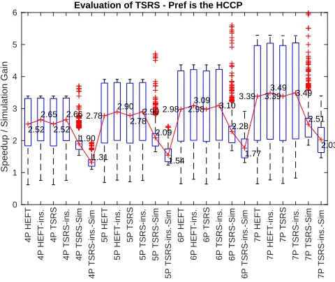
Figure 1. Evaluation of TSRS (972different DAGs)
1) Evaluating TSRS: In this Subsection, TSRS is
eval-uated. The results are illustrated by using boxplots in Matlab. The (’Sim’,’ins.’) in the x-axis of Fig. 1 indi-cate simulation gain and insertion policy, respectively. In Fig. 1, 972 different DAGs have been used (all different fat, regularity, density and jump combinations) with n =
100,CCR = [0.1,0.5,2,10], βw = βc = [0.5,1,1.5] as
well as several processor configurations. The ’4P’ indicates 4 different single-core processors. In this subsection, all the processors are either single-cores or co-processors. The
TSRS makespan is approximately the same as that of the standalone HEFT, in all cases. Furthermore, both HEFT and TSRS perform better by using the insertion scheduling pol-icy but the gains are small. By using the insertion scheduling policy lower simulation gain values occur because in that case the number of computation costs needed is higher.
0 10 20 30 40 50 60 70 80 90
DAGs
0 1 2 3 4 5 6
Speedup
0 1 2 3 4 5 6 7 8 9 10
Simulation Gain
D.P=(0,0,1,1,1,1,0,0,0),C.P=(0,0,1,1,1,1,0,0,0),cores=(0,0,4,4,6,6)
SHEFT MHEFT TSRS+METS TSRS+METS(Sim)
Figure 2. METS with TSRS (n= 100,CCR= 0.5,βw=βc= 0.5)
2) Evaluating METS with TSRS: In this Subsection,
METS with TSRS is evaluated (Fig. 2, Fig. 3) - pref = 6 in all cases. Given that HEFT algorithm doesn’t include multi-threading, we have implemented HEFT to use a) ST implementations only (SHEFT) and b) maximum thread implementations only (MHEFT). In this Subsection we have evaluated METS without using the insertion scheduling policy because the makespan improvement is not significant comparing to the simulation loss. Therefore, by using the insertion scheduling policy, METS achieves slightly better makespan values than those shown in Fig. 2-Fig. 4; stan-dalone METS gives better makespan values, as in Algo-rithm 4 theM(i)values are computed by using median core utilization factor values and not the real ones. SHEFT and MHEFT use the insertion scheduling policy.
In Fig. 2, a total of 81 different DAGs is considered com-bining fat, regularity, density and jump. The first 27 DAGs refer to skinny DAGs, the next 27 to medium fat and the last 27 DAGs refer to fat DAGs. As it can be observed, skinny DAGs give low speedup but high simulation gain values, while fat DAGs give high speedup but lower simulation gain values. SHEFT is more efficient than MHEFT when the task parallelism is high, as by providing more cores, more tasks are executed in parallel. On the other hand, when the task parallelism is low, MHEFT gives always higher speedup values, as it is preferable to use less processors but with high CC. It is important to note that our method follows the trend of the best of the two.
[image:9.612.57.297.369.571.2]CCR = [0.1,0.2,0.5,1,2,5,10] (3402 different DAGs in total) and four different processor configurations. When only multi-core processors are used, the heuristics given in Subsection IV-B perform very well and give significant speedup values. On the other hand, when fast coprocessors are used apart from multi-core processors, the heuristics given in Subsection IV-B perform better than both SHEFT and MHEFT but the gain is low. The reason lies in the fact that HEFT is a greedy algorithm as it always chooses the processor giving the minimum EFT value; therefore, the coprocessors never become idle and push aside the multi-core processors; thus, most of the tasks are executed on the coprocessors. This is why all three methods give close makespan values. ’T SRS∗’ refers to theT SRSwhen the last loop kernel in Algorithm 3 is used (at least one coprocessor exists). The last loop kernel in TSRS reduces the number of simulations on the HCCP group. In the left bottom figure, the makespan degradation in ’T SRS∗’ is larger because the HCCP group contains 2 processors and therefore excluding the group from SL means that none of the two coprocessors is used. As far as the simulation gain is concerned, it is lower when coprocessors exist because most of the tasks are simulated on the coprocessors while pref = 6; in this case a larger number of extra simulations occurs. On the other hand, when no coprocessor exists,pref is a HCCP and therefore it is the most preferable processor, meaning that the number of extra simulations is reduced.
C. Real World Applications
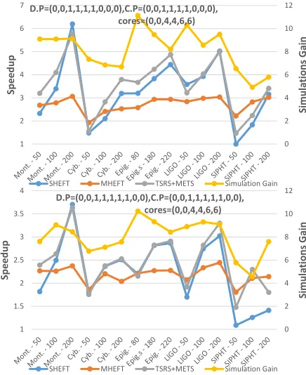
TSRS and METS have been evaluated to Montage, Cy-berShake, Epigenomics, LIGO and SIPHT real world ap-plications [19] [20]. We have used small, medium and large graphs for each one of the 5 applications (from 50 up to 200 tasks, Fig. 4) as well as real communication and computation costs forwt,pref,1, taken from [19] [20]. The computation
costs for the other processors have been selected as random values within a range as in Subsection V-B. SHEFT performs better than MHEFT when the number of processors is low (as in Fig. 4), as in that case SHEFT uses 20 cores while MHEFT uses 4 processors. However, by increasing the number of the processors MHEFT outperforms SHEFT (our method follows the trend of the best of the two). Moreover, when no coprocessor is used, METS performs better for the reason explained in the previous subsection. Last, Epigenomics and SIPHT are less scalable.
VI. CONCLUSIONS ANDFUTUREWORK
TSRS modifies HEFT’s processor selection phase in order to discard all the processors which cannot minimize the heuristic cost function, regardless of their computation costs; this way, the DAG computation costs required by HEFT become limited. Although TSRS, never excludes a processor minimizing the heuristic cost function (here EFT), it slightly affects the task priority list. However, the results show that for monotonic computation costs the output makespan is not
SHEFT MHEFT TSRS+METS TSRS+METS(Sim) 0 5 10 15 20
25 Speedup / Simulation Gain
D.P=(1,1,1,1,1,1,0,0,0),C.P=(2,2,2,2,2,2,0,0,0),cores=(2,2,4,4,6,6) 3.1538 3.5493 3.7701 11.3774 SHEFT MHEFT TSRS+METS TSRS+METS(Sim) 0 2 4 6 8 10 12 14 16 18 20
Speedup / Simulation Gain
D.P=(0,0,1,1,1,1,0,0,0),C.P=(0,0,1,1,1,1,0,0,0),cores=(0,0,4,4,6,6) 2.5213 2.2798 2.801 9.1225 SHEFT MHEFT TSRS+METS TSRS*+METS TSRS+METS(Sim) TSRS*+METS(Sim) 0 2 4 6 8 10 12 14 16 18
Speedup / Simulation Gain
D.P=(1,1,1,1,1,1,1,0,0),C.P=(2,2,2,2,2,2,2,0,0),cores=(2,2,4,4,6,6) 2.7356 2.8756 2.8777 2.7581 8.7272 10.4071 SHEFT MHEFT TSRS+METS TSRS*+METS TSRS+METS(Sim) TSRS*+METS(Sim) 0 2 4 6 8 10 12 14 16
18 Speedup / Simulation Gain
[image:10.612.314.563.75.394.2]D.P=(0,0,1,1,1,1,1,0,0),C.P=(0,0,1,1,1,1,1,0,0),cores=(0,0,4,4,6,6) 1.9106 1.8348 1.9136 1.9131 7.2442 8.7635
Figure 3. Evaluation of METS with TSRS (3402different DAGs)
0 2 4 6 8 10 12 1 2 3 4 5 6 7 S im u la ti o n s G a in S p e e d u p D.P=(0,0,1,1,1,1,0,0,0),C.P=(0,0,1,1,1,1,0,0,0), cores=(0,0,4,4,6,6)
SHEFT MHEFT TSRS+METS Simulation Gain
0 2 4 6 8 10 12 1 1.5 2 2.5 3 3.5 4 S im u la ti o n s G a in S p e e d u p D.P=(0,0,1,1,1,1,1,0,0),C.P=(0,0,1,1,1,1,1,0,0), cores=(0,0,4,4,6,6)
SHEFT MHEFT TSRS+METS Simulation Gain
[image:10.612.329.547.429.696.2]degraded; as in [15], we show that the meanRanku compu-tation costs is not the best choice. The insertion scheduling policy is not preferred as the makespan improvement is not significant comparing to the simulation loss.
METS refers to heuristics finding which tasks are going to be split into multiple threads as well as the number of threads used, without requiring all the computation costs in the DAG. We evaluated METS with TSRS without using the insertion scheduling policy, as the makespan improvement is not significant comparing to the simulation loss. Standalone METS gives better makespan values.
In our future work, we intend to extend METS with heuristics finding whether a multi-core processor or a co-processor is more efficient for the current task (we believe this will give better makespan values when fast coprocessors are used). Our future work also includes the application and evaluation of both TSRS and METS to other TS algorithms such as HCPT, HPS, PETS, CPOP and others. Furthermore, we aim to develop a tool that takes OmpSs (Barcelona Supercomputing Center programming model) C-code as input and by using both TSRS and METS, it outputs a good quality schedule in low time. We use OmpSs as it extends OpenMP with new directives to support GPUs and FPGAs.
ACKNOWLEDGMENT
This work is partly supported by the European Commis-sion under H2020-ICT-20152 contract 687584 - Transparent heterogeneous hardware Architecture deployment for eN-ergy Gain in Operation (TANGO) project.
REFERENCES
[1] E. Ilavarasan and P. Thambidurai, “Low complexity perfor-mance effective task scheduling algorithm for heterogeneous
computing environments,” Journal of Computer Sciences,
vol. 3, pp. 94–103, 2007.
[2] H. Arabnejad and J. G. Barbosa, “List scheduling algorithm
for heterogeneous systems by an optimistic cost table,”IEEE
Trans. Parallel Distrib. Syst., vol. 25, no. 3, pp. 682–694, Mar. 2014.
[3] H. Topcuouglu, S. Hariri, and M.-y. Wu, “Performance-effective and low-complexity task scheduling for
heteroge-neous computing,”IEEE Trans. Parallel Distrib. Syst., vol. 13,
no. 3, pp. 260–274, Mar. 2002.
[4] T. Hagras and J. Janecek, “A simple scheduling heuristic for
heterogeneous computing environments,” in2nd International
Conference on Parallel and Distributed Computing, ser. IS-PDC’03, 2003, pp. 104–110.
[5] E. Ilavarasan, P. Thambidurai, and R. Mahilmannan, “High performance task scheduling algorithm for heterogeneous
computing system,” in Conference on Algorithms and
Ar-chitectures for Parallel Processing, ser. ICA3PP, 2005, pp. 193–203.
[6] M. I. Daoud and N. Kharma, “A high performance algo-rithm for static task scheduling in heterogeneous distributed
computing systems,” Journal of Parallel and Distributed
Computing, vol. 68, no. 4, pp. 399 – 409, 2008.
[7] E. Saule, D. Bozda˘g, and U. V. Catalyurek, “A moldable online scheduling algorithm and its application to parallel
short sequence mapping,” in Job Scheduling Strategies for
Parallel Processing, ser. JSSPP, 2010, pp. 93–109.
[8] E. Deelman, G. Singh, M.-H. Su, J. Blythe, Y. Gil, C. Kessel-man, G. Mehta, K. Vahi, G. B. BerriKessel-man, J. Good, A. Laity, J. C. Jacob, and D. S. Katz, “Pegasus: A framework for map-ping complex scientific workflows onto distributed systems,”
Sci. Program., vol. 13, no. 3, pp. 219–237, Jul. 2005.
[9] J. Meng, X. Wu, V. Morozov, V. Vishwanath, K. Kumaran, and V. Taylor, “Skope: A framework for modeling and
exploring workload behavior,” inComputing Frontiers (CF),
2014, pp. 6:1–6:10.
[10] C. Augonnet, S. Thibault, R. Namyst, and P.-A. Wacrenier, “Starpu: A unified platform for task scheduling on
heteroge-neous multicore architectures,” Concurrency and
Computa-tion: Practice & Experience, vol. 23, pp. 187–198, 2011.
[11] O. Beaumont, L. Eyraud-Dubois, and S. Kumar, “Approxima-tion Proofs of a Fast and Efficient List Scheduling Algorithm for Task-Based Runtime Systems on Multicores and GPUs,” in Parallel & Distributed Processing Symposium, 2017.
[12] C. Boeres, J. V. Filho, and V. E. F. Rebello, “A cluster-based strategy for scheduling task on heterogeneous processors,” in Computer Architecture and High Performance Computing Symposium, ser. SBAC-PAD, 2004, pp. 214–221.
[13] S. Kedad-Sidhoum, F. Monna, G. Mouni´e, and D. Trystram, “Scheduling independent tasks on multi-cores with gpu
accel-erators,” in Euro-Par 2013: Parallel Processing Workshops,
2014, pp. 228–237.
[14] L. F. Bittencourt, R. Sakellariou, and E. R. M. Madeira, “Dag scheduling using a lookahead variant of the heterogeneous
earliest finish time algorithm,” in Parallel, Distributed and
Network-based Processing conference, 2010, pp. 27–34.
[15] H. Zhao and R. Sakellariou, “An experimental investigation into the rank function of the heterogeneous earliest finish
time scheduling algorithm,” in 9th International Euro-Par
Conference Klagenfurt, 2003, pp. 189–194.
[16] S. Baskiyar and P. SaiRanga, “Scheduling directed a-cyclic task graphs on heterogeneous network of workstations to
minimize schedule length,” inParallel Processing Workshops,
11 2003, pp. 97– 103.
[17] C. Hui, “A high efficient task scheduling algorithm based
on heterogeneous multi-core processor,” in2nd International
Workshop on Database Technology and Applications (DBTA). IEEE, 2010.
[18] F. Suter, “Daggen: A synthethic task graph generator,” https://github.com/frs69wq/daggen, 2012, accessed: 2017-12.
[19] G. Mehta and G. Juve. (2014) Workflow generator. https://confluence.pegasus.isi.edu/display/pegasus/WorkflowGenerator. Accessed: 2017-12.
[20] G. Juve, A. Chervenak, E. Deelman, S. Bharathi, G. Mehta, and K. Vahi, “Characterizing and profiling scientific
work-flows,”Future Gener. Comput. Syst., vol. 29, no. 3, pp. 682–