This is a repository copy of
An expectation maximisation algorithm for behaviour analysis
in video
.
White Rose Research Online URL for this paper:
http://eprints.whiterose.ac.uk/91449/
Version: Accepted Version
Proceedings Paper:
Isupova, O., Mihaylova, L., Kuzin, D. et al. (2 more authors) (2015) An expectation
maximisation algorithm for behaviour analysis in video. In: 18th International Conference
on Information Fusion (Fusion), 2015. 18th International Conference on Information
Fusion, 6-9 July 2015, Washington D.C (USA). IEEE , 126 - 133. ISBN 978-0-9824-4386-6
[email protected] https://eprints.whiterose.ac.uk/ Reuse
Unless indicated otherwise, fulltext items are protected by copyright with all rights reserved. The copyright exception in section 29 of the Copyright, Designs and Patents Act 1988 allows the making of a single copy solely for the purpose of non-commercial research or private study within the limits of fair dealing. The publisher or other rights-holder may allow further reproduction and re-use of this version - refer to the White Rose Research Online record for this item. Where records identify the publisher as the copyright holder, users can verify any specific terms of use on the publisher’s website.
Takedown
If you consider content in White Rose Research Online to be in breach of UK law, please notify us by
An Expectation Maximisation Algorithm for
Behaviour Analysis in Video
Olga Isupova, Lyudmila Mihaylova, Danil Kuzin
Department of Automatic Control and Systems Engineering, University of Sheffield Sheffield, UK
Email: [email protected], [email protected], [email protected]
Garik Markarian
School of Computing and Communications, Lancaster University Lancaster, UK
Email: [email protected]
Francois Septier
Institut Mines-Telecom, Telecom Lille Villeneuve d’Ascq Cedex, France Email: [email protected]
Abstract—Surveillance systems require advanced algorithms able to make decisions without a human operator or with minimal assistance from human operators. In this paper we propose a novel approach for dynamic topic modeling to detect abnormal behaviour in video sequences. The topic model de-scribes activities and behaviours in the scene assuming behaviour temporal dynamics. The new inference scheme based on an Expectation-Maximisation algorithm is implemented without an approximation at intermediate stages. The proposed approach for behaviour analysis is compared with a Gibbs sampling inference scheme. The experiments both on synthetic and real data show that the model, based on Expectation-Maximisation approach, outperforms the one, based on Gibbs sampling scheme.
I. INTRODUCTION
The amount of CCTV cameras has significantly grown over the last decades. The rough estimates indicate that there are about 5 million cameras in the UK alone. However, the processing of data generated by CCTV systems is inefficient due to the vast volume. The automatic video analytic systems are required to help in analysing this data. There are a number of requests which ideally should be answered by such systems: “What is going on in the area? What are the typical motion patterns? What kind of abnormality is observed?” The latter question has to be answered in real-time to warn a human operator to respond.
The area of abnormal behaviour detection has become very attractive to the researchers over the last decade. One of the challenges is to determine what abnormality is. Some authors elicit exact patterns for normal behaviours and consider ev-erything that is not similar to those patterns as abnormal. In [1] the normal patterns are built by clustering the visual features extracted from the video. The anomaly decision rule is then based on the comparison between a new observation and the nearest pattern. In [2] the similar approach based on the Hidden Markov Model for each of the normal cluster is presented. The Sparse Reconstruction Cost measure for abnor-mality is proposed in [3]. The idea is that normal behaviour is well represented on the basis built from the training data
(consisting only of the normal behaviour patterns) and has a sparse coefficient vector. It is assumed that abnormal behaviour description cannot be explained with the normal patterns and it has a dense coefficient vector.
Another approach to determine the abnormality is to con-sider a statistically rare event as abnormal. The models then rely on statistical regularities, training one-class classifiers such as one-class Support Vector Machine (e.g. [4]) or topic models (e.g. [5]). Topic models identify features appearing together, forming typical activities of the scene. A number of variations of the convential topic models were proposed recently. In [6] the authors assume that distributions over these activities can be clustered. Temporal dependence among the activities is considered in [7], [8]. The continuous model for an object velocity is proposed in [9]. The comparison of different abnormality measures for such kind of models is presented in [10].
The advantage of the topic modeling approach for the abnor-mal behaviour detection is that topic models can automatically discover meaningful activities [11]. The detection of abnormal-ity can be performed within a probabilistic framework, where events which cannot be explained by learnt probability model are considered as abnormal.
Topic modeling was originally developed for text min-ing [12], [13]. The idea is that documents can be represented as distributions over topics where topics are distributions over words. In video applications clips can be treated as documents and features extracted from the video are treated as visual words. Discovered topics can be interpreted as activities supposing that there is a fixed number of such activities shared by all the clips.
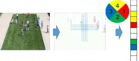
Figure 1. Visual feature extraction process: from an input frame (on the left) an optical flow is calculated (in the centre); the optical flow is averaged within the cells and quantised into four directions to get the feature representation (on the right)
– Latent Dirichlet Allocation (LDA) [13] and Probabilistic Latent Semantic Analysis (PLSA) [12]. In [7] the LDA-based model is developed. We propose the PLSA-LDA-based model for behaviour analysis and abnormality detection with the similar generative model. The abnormality measure is based on the likelihood of new observations calculated with learnt probabilistic distributions. The proposed inference scheme is based on the maximum likelihood approach. The derivation of the proposed approach can be done without additional approximations.
This paper goes beyond the current state-of-the-art in several directions: (i) a PLSA-based model for behaviour analysis is proposed; (ii) a new inference scheme is designed based on the maximum likelihood approach. An Expectation-Maximisation (EM) algorithm is developed for the optimisation problem. (iii) The proposed EM-algorithm for behaviour analysis is compared with the Gibbs sampling algorithm presented in [7]. More accurate results for the EM-algorithm are demonstrated. The rest of the paper is organised as follows. First the description of the visual features treated as visual words is presented in Section II. Section III provides the brief review of Markov Clustering Topic Model proposed in [7] while Section IV explains the proposed model. The abnormality detection procedure and summary of the whole approach is discussed in Section V. Section VI demonstrates the exper-imental results. The conclusion of the paper is presented in Section VII.
II. VISUALFEATURES
In this paper the local motions are treated as the visual features. Each frame is divided into small cells of sizeN×N pixels. For each of the cells the mean optical flow over all pixels forming this cell is calculated. If the optical flow is higher than a threshold (in order to remove noise false detections) this cell is considered as moving and its motion is quantised into four directions. The visual word is then formed by a position of the moving cell and a direction of its motion (Fig. 1). Thereby the vocabulary size is Number of cells×4. The documents for the topic model are the short video clips of 1 second length uniformly selected from the whole video sequence.
III. MARKOVCLUSTERINGTOPICMODEL
The authors of Markov Clustering Topic Model (MCTM) [7] propose two novelties compared to the standard Latent Dirichlet Allocation (LDA) topic model [13]. First, the topic distributions for the documents are considered to be exactly the same for the different documents. Moreover, there are only a limited number of the different topic distributions, called behaviours in [7], and each document within a dataset corresponds to one of these behaviours. The topics representing visual word distributions are assumed to explain simple actions while the behaviours are assumed to explain more complex interactions within a scene. Furthermore, the behaviour contains all information about the scene as it is responsible for all the actions appearing within the scene and the actions determine the visual words composing the scene. Second, the MCTM assumes that changes between the different behaviours happen relatively rarely, that each behaviour lasts for some time (during some number of sequential clips). This assumption is modelled with the Markov property.
The motivation of these assumptions can be seen with the following data. Let us assume that we have a fixed camera on a road junction regulated by traffic lights. Video data obtained from this camera has strict periodical motions. Each traffic light regime corresponds to a behaviour as these regimes follow each other with the given order and they explain all the actions happening within the scene.
LetX denote the set of all the visual words, i.e. locations and directions of primitive motion, Y – the set of all the actions (topics), distributions over the visual words, i.e. some simple small group motion like motion to the right in the small area of the scene, Z – the set of all the behaviours, distributions over the actions (topics), i.e. some complex motion like general right-flow traffic or turning to the left on the junction governing by the particular traffic light regime. Let φ denote the matrix of the visual word distributions for the actions (topics),θdenote the matrix of the action distributions for the behaviours and ψ denote the matrix of the transition probabilities between the behaviours:
φ={φx,y}x∈X,y∈Y, φx,y =p(x|y), φy={φx,y}x∈X;
θ={θy,z}y∈Y,z∈Z, θy,z=p(y|z), θz={θy,z}y∈Y;
ψ={ψz,z˜ }z˜∈Z,z∈Z, ψz,z˜ =p(˜z|z), ψz={ψz,z˜ }z˜∈Z,
wherez– is the ‘start’ behaviour,z˜– is the ‘final’ behaviour. The generative model can be described then as follows: for each clip t a behaviour zt is sampled according to the
behaviour for the previous clipzt−1 fromψzt
−1. Then forNt (the length of the cliptin the visual words) times the following process is repeated: an action yi,t is sampled according to
the behaviour zt from θzt, a visual word xi,t is sampled
according to the actionyi,t from φyi,t,i={1, . . . , Nt}. The
pairs (xi,t, yi,t) given zt for all clips t and all tokens i are
LDA the Dirichlet prior distributions are considered for all discrete distributions:
p(φy|β) =Dir(φy;β);
p(θz|α) =Dir(θz;α);
p(ψz|γ) =Dir(ψz;γ),
whereDirdenotes a Dirichlet distribution andβ,α,γare the corresponding hyperparameters.
IV. THE PROPOSED APPROACH
A. Motivation
The inference for MCTM in [7] is based on the collapsed Gibbs sampler. The Markov chain is built to sample the hidden variables from the joint distribution of all the actions and the behaviours given the data. The Gibbs sampling update for the actionyi,t and the behaviour zt is derived by integrating
out the parameters φ, θ and ψ. For the behaviour update step integrating out the transition matrixψuses the following assumption:
p(zt|y\t,z\t)∝
∝
Z
p(zt|zt−1,ψ)p(zt+1|zt, ψ)p(ψ|z\t)dψ, (1)
wherey\t denotes all the actions in the data excluding those corresponding to the clip t,z\t denotes all the behaviours in
the data excluding that corresponding to the clip t. While the exact formula is as follows:
p(zt|y\t,z\t) =
=
Z p(z
t|zt−1,ψ)p(zt+1|zt,ψ) P
˜
zt∈Z
p(˜zt|zt−1,ψ)p(zt+1|z˜t,ψ)
p(ψ|z\t)dψ (2)
One can notice that in this case the sign∝does not mean, as usual, the precision up to a normalization constant.
B. Solution
In order to infer the model without such kind of approxi-mations we propose a new inference scheme for the model. The MCTM is developed from one of two base topic models – LDA [13], while we would like to use the other base topic model – PLSA [12]. PLSA is a simpler model which does not assume any prior distributions and treats onlyφandθmatrices as parameters and utilises maximum likelihood estimates for them applying the EM-algorithm. PLSA can be considered as a special case of LDA [14]. Moreover, experiments on real data show that PLSA and LDA have compatible results [15]. Most of the LDA-based topic models can be reformulated as PLSA-based models with simpler parameter inference [16]. Since the PLSA model has the more straightforward inference we use the PLSA-based MCTM (denoted as EM-MCTM) without approximations at the intermediate stages.
C. EM-MCTM
The generative model for the PLSA-based MCTM is the same as for the MCTM [7] except for: (a) one more model parameter π = {πz}z∈Z – the distribution for the initial
behaviourz1is introduced, and (b) the algorithm does not rely
on prior distributions for any of the parameters{π,φ,θ,ψ}. Details can be found in Algorithm IV.1
Algorithm IV.1The generative model for EM-MCTM
Require: The number of clips –T, the length of each clip – Nt ∀t={1, . . . , T}, the parameters – π,φ,θ,ψ; Ensure: The datasetx1:T ={x1,1, . . . , xi,t, . . . , xNT,T};
1: for all t∈ {1, . . . , T}do
2: if t= 1 then
3: draw a behaviour for the clip from the initial distri-bution: zt∼π;
4: else
5: draw a behaviour for the clip based on the behaviour of the previous clip: zt∼ψzt−1;
6: for all i∈ {1, . . . , Nt} do
7: draw an action for the token i based on the chosen behaviour:yi,t ∼θzt;
8: draw a visual word for the token i based on the chosen action:xi,t ∼φyi,t;
The model parameters{π,φ,θ,ψ} are estimated with the maximum likelihood approach. The EM-algorithm [17] is applied to the optimisation problem. The full likelihood of the model is as follows:
p(x1:T,y1:T,z1:T|π,φ,θ,ψ) =p(z1|π)
"T Y
t=2
p(zt|zt−1,ψ)
#
×
T Y
t=1
Nt
Y
i=1
p(xi,t|yi,t,φ)p(yi,t|zt,θ), (3)
where T – is the number of clips, x1:T =
{x1,1, . . . , xi,t, . . . , xNT,T} – is the sequence of all visual
words in the dataset, y1:T ={y1,1, . . . , yi,t, . . . , yNT,T} – is
the sequence of all actions in the dataset,z1:T ={z1, . . . , zT}
– is the sequence of all behaviours in the dataset.
Since there is Markov dependence in the data, the derivation of the EM-algorithm is similar to the EM-algorithm applied to the Hidden Markov Model known as the Baum-Welch algorithm [18]. Following the idea of the Baum-Welch algo-rithm, the additional variablesα˜z,tandβ˜z,tfor each behaviour
z and each clip t are introduced in the E-step. They are calculated efficiently by recursive expressions. Knowing these additional variables and the current estimates of the model parameters, the posterior estimates of the hidden variables can be computed. The full E-step then can be written as follows:
˜
αz,t= Nt
Q
i=1
P
y∈Y
φxi,t,yθy,z
P
˜
z∈Z ˜
α˜z,t−1ψz,z˜,ift>2;
˜
αz,1=πz N1
Q
i=1
P
y∈Y
φxi,1,yθy,z;
˜
βz,t= P
˜
z∈Z ˜
βz,t˜ +1ψ˜z,z Nt+1
Q
i=1
P
y∈Y
φxi,t+1,yθy,z˜,ift6T−1;
˜
βz,T = 1;
(5) p(z|x1:T)∝α˜z,tβ˜z,t; (6)
p(zt, zt−1|x1:T)∝α˜zt−1,t−1β˜zt,tψzt,zt−1 ×
Nt
Y
i=1
X
y∈Y
φxi,t,yθy,zt;
(7)
p(yi,t, zt|x1:T)∝φxi,t,yi,tθyi,t,ztβ˜zt,t
X
˜
z∈Z ˜
αz,t˜ −1ψzt,˜z
×
Nt
Y
j=1
j6=i X
˜
y∈Y
φxj,t,y˜θy,z˜ tift>2;
p(yi,1, z1|x1:T)∝φxi,1,yi,1θyi,1,z1β˜z1,1πz1 ×
N1
Y
j=1
j6=i X
˜
y∈Y
φxj,1,˜yθy,z˜ 1;
(8) p(yi,t|x1:T) =
X
z∈Z
p(yi,t, z|x1:T) (9)
Having the posterior estimates of the hidden variables, the estimates of the model parameters are easily calculated during the M-step:
πz=
p(z1=z|x1:T) P
˜
z
p(z1= ˜z|x1:T)
; (10)
φx,y = T P t=1 Nt P i=1
p(yi,t =y|x1:T)δxi,t,x
T P t=1 Nt P i=1
p(yi,t=y|x1:T)
; (11)
θy,z= T P t=1 Nt P i=1
p(yi,t =y, zt=z|x1:T)
T P t=1 Nt P i=1 P ˜ y
p(yi,t= ˜y, zt=z|x1:T)
; (12)
ψz,z˜=
T P
t=2
p(zt=z, zt−1= ˜z|x1:T)
T P
t=2
P
z′
p(zt=z, zt−1=z′|x1:T)
, (13)
whereδ·,·- is the Kronecker delta, x,y,zwithout subscripts denote the possible values for a word, an action and a behaviour variable, respectively, and the same symbols with subscript denote realisations in a particular place in the dataset.
V. ABNORMALITY DETECTION
Following the approach proposed in [7] we consider the sim-ilar framework for abnormality detection. A certain number, Ttr clips is used as a training dataset for parameter inference.
The training dataset is assumed to be representative, i.e. that no more adaptation of the parameters is required when new clips are available. After the training stage we obtain the estimates
{φ,ˆ ˆθ,ψ}ˆ of the model parameters and use these estimates to evaluate whether testing clips are normal or abnormal.
The measure of abnormality is defined as a likelihood of a new clip xt+1 = {x1,t+1, . . . , xNt+1,t+1} given all the previous clips till the clip t inclusively x1:t = {x1, . . . ,xt}
and the estimates{φ,ˆ ˆθ,ψ}ˆ of the model parameters obtained from the training stage:
p(xt+1|x1:t,φ,ˆ θ,ˆ ψˆ) = X
zt
X
zt+1
h
p(xt+1|zt+1,φ,ˆ θˆ)
×p(zt+1|zt,ψˆ)p(zt|x1:t,φ,ˆ θ,ˆ ψˆ) i
, (14) where the predictive behaviour probability given the data sequence can be calculated recursively as follows:
p(zt|x1:t,φ,ˆ ˆθ,ψˆ) =
=X
zt−1
p(xt|zt,φ,ˆ θˆ)p(zt|zt−1,ψˆ)p(zt−1|x1:t−1,φ,ˆ ˆθ,ψˆ)
p(xt|x1:t−1,φ,ˆ θ,ˆ ψˆ)
(15) In order to compare the likelihood of different clips, con-taining a different number of visual words, the normalised likelihoodsis calculated as the final measure of abnormality:
logs(xt+1|x1:t) = 1
Nt+1
logp(xt+1|x1:t). (16)
When this normalised likelihood is lower than a threshold, the clip xt+1 is supposed to be abnormal, i.e. some kind of
abnormal behaviour happens during this clip. It can be a rare visual word xi,t+1; or a rare combination of visual words
which can not be explained with any of the learnt actions (topics); or a combination of visual words can form the learnt actions (topics), but the combination of the actions is rare; or a sequence of behaviours which conflicts with the learnt behaviour dynamics.
The full learning and detection procedure of the EM-MCTM can then be described as follows. Ttr clips from the whole
(a) (b)
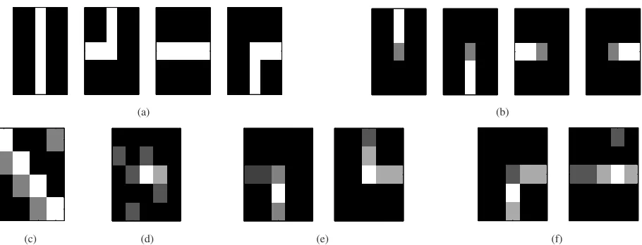
[image:6.595.77.532.101.275.2](c) (d) (e) (f)
Figure 2. Synthetic data example (the lighter elements correspond to the higher probabilities): (a) The true behaviour representations in visual words; (b) the true actions (topics) representations in visual words; (c) the true transition probability matrix for behaviour dynamics – columns correspond to start behaviours, rows correspond to final behaviours; (d) an example of an abnormal ‘clip’ with the type of abnormality – abnormal word joint appearance; (e) examples of abnormal ‘clips’ with the type of abnormality – abnormal action joint appearance; (f) an example of an abnormal ‘clip’ with the type of abnormality – abnormal behaviour dynamics, where the left ‘clip’ is normal and the right ‘clip’ is abnormal as the ‘right-down’ motion should be followed by the ‘vertical’ flow, not the ‘horizontal’ one
VI. EXPERIMENTS
In this section we apply the proposed EM-MCTM approach for abnormality detection and compare it with the MCTM based on the Gibbs sampling scheme inference proposed in [7] (denoted later as GS-MCTM). First, we illustrate the models with synthetic data and then apply them to real video data.
It is worth noting that the EM-algorithm depends on the initialisation. Although the Gibbs sampling algorithm does not depend on the initialisation, due to randomness of the process the results of several runs can slightly differ. For all experiments we use random initialisations and show average results over 20 runs for each algorithm with the same data and different initialisations.
For quantitative evaluation we compare the answers of the models with the given ground truth. Two kinds of classification accuracy measures are used: the error percentage and the f-measure. Theerror percentageis a fraction of the model an-swers that are not equal to the ground truth. Thef-measure[19] is a harmonic mean of precision and recall, where precision is a fraction of model detections that are correct (in terms of the ground truth) and recall is a fraction of the ground truth positive cases that are detected by the model.
A. Synthetic data
We use synthetic data to show the models performance. Let us assume that we observe a road junction with the following type of motions: the ‘vertical’ traffic flow, the ‘left-up’ turning, the ‘horizontal’ traffic flow, and the ‘right-down’ turning (Fig. 2a). Each of the motion type we model as a behaviour. Each of the behaviours are modelled to consist of two actions (topics) forming four actions in total (Fig. 2b). The transition probability matrix can be found on Fig. 2c.
Having these distributions for the behaviours, the actions (topics), and the behaviour dynamics, we can generate ‘clips’
from our generative model (we use the uniform distribution for the initial behaviour probability). We add some small noise to all the distribution matrices and generate 1000 ‘clips’ as a training dataset.
We also generate 1000 testing ‘clips’ where we randomly include 300 ‘abnormal’ ones. Three kinds of abnormality is used with an equal probability for the generation of ‘abnormal clips’:
(a) abnormal word joint appearance. On step 8 of Algo-rithm IV.1 we add a significant noise to the words in actions (topics) distribution matrix φ obtained a ‘clip’ consisted of the words, rarely appearing together, or even the new words in comparison with the training dataset (Fig. 2d for example);
(b) abnormal action joint appearance. On step 7 of Al-gorithm IV.1 we sample actions (topics) not from the existing actions in the behaviour distributionθzt, where
zt is the behaviour for the current ‘clip’ but we sample
actions from one of two ‘abnormal’ behaviours (Fig. 2e) obtained the ‘clip’ containing the actions, which have never been together in the training dataset;
(c) abnormal behaviour dynamics. On step 5 of Algo-rithm IV.1 we sample a behaviour for the current ‘clip’ having the minimum probability in the transition distri-bution from the behaviour for the previous ‘clip’ ψzt
−1
obtained unusual behaviour dynamics from the ‘clip’t−1
to the ‘clip’t (Fig. 2f for example).
We run the EM-MCTM with 100 iterations, the GS-MCTM with 200 burn-in iterations, followed with 500 iterations taking 5 independent samples with lag of 100 iterations, the Dirichlet hyperparameters are symmetric and fixed as {α = (5, . . . ,5),β = (1
5, . . . , 1
5),γ = (1, . . . ,1)}. Each
Reference
a
c
t
io
n
1
a
c
t
io
n
2
a
c
t
io
n
3
a
c
t
io
n
4
GS-MCTM 1 GS-MCTM 2 EM-MCTM 1 EM-MCTM 2
(a)
Reference
b
e
h
a
v
io
u
r
1
b
e
h
a
v
io
u
r
2
b
e
h
a
v
io
u
r
3
b
e
h
a
v
io
u
r
4
GS-MCTM 1 GS-MCTM 2 EM-MCTM 1 EM-MCTM 2
(b) Reference GS-MCTM 1 GS-MCTM 2 EM-MCTM 1 EM-MCTM 2
[image:7.595.319.555.443.531.2](c)
Figure 3. Comparison of the learnt parameters by the models with the true reference parameters from the synthetic data example: (a) Actions (topics) restoration comparison; (b) Behaviours restoration comparison; (c) Transition probability matrix for behaviour dynamics restoration comparison. From the left column to the right one: the reference true distributions; the restored distributions by the ‘best’ Gibbs sampling MCTM (GS-MCTM 1) algorithm run; the restored distributions by the ‘worst’ Gibbs sampling MCTM (GS-MCTM 2) algorithm run; restored distributions by the ‘best’ EM-algorithm for MCTM (EM-MCTM 1) run; the restored distributions by the ‘worst’ EM-algorithm for MCTM (EM-MCTM 2) run
1) Parameter Learning: We can qualitatively evaluate how the models restore the references parameters {φ,θ,ψ}. We choose the ‘best’ and the ‘worst’ run among 20 runs for each model and present the comparison between the restored parameters and the reference ones. For the Gibbs sampling model for this illustrative purpose we use the estimation of the parameters obtained by the last sample of the Markov Chain. Figure 3a demonstrates the comparison for the words in actions (topics) distributions φ. One can notice that while the best runs for both models restore the parameters quite well, the worst runs for both models do not have such good results. In this case the algorithms extract true behaviours as learnt topics. Indeed, given only observed data (visual words) it is impossible to distinguish between two possible outcomes: two true topics and true behaviour consisting of these two topics and one topic equal to true behaviour and behaviour consisting of this topic. The similar results can be found for the actions (topics) in behaviours distributionsθ (Fig. 3b). Although the transition probability matrix for the behaviour dynamics ψ is restored quite well for all cases (the worst run of the EM-MCTM has slightly worse results as it does not distinguish the ‘horizontal’ and the ‘right-down’ traffic behaviours) (Fig. 3c).
2) Classification of abnormality: We use the trained models to classify the testing data into two classes – normal or abnormal, and compare the classification answers with the ground truth known after the generation. For the GS-MCTM we used two kinds of likelihood to measure abnormality of a clip: (a) the proposed conditional likelihood (16) given the learnt parameters {φ,ˆ ˆθ,ψ}ˆ obtained from the last sample of
Table I
THE CLASSIFICATION RESULTS FOR THE SYNTHETIC EXAMPLE
Quality measure
Reference parameter model
GS, Marginalized likelihood
GS, Conditional likelihood
EM
mean error
percentage 0.0860 0.1503 0.1495 0.1387
mean
f-measure 0.9404 0.8961 0.8962 0.9035
the Markov Chain [20] and (b) the marginal likelihood, where the integral over parameters is approximated with a sum of the Gibbs samples (the saliency measure used in [7]). We also perform the classification for the model using the reference parameters and the conditional likelihood for the abnormality measure to show the best results that can be achieved if topic models are able to ideally restore the parameters {φ,θ,ψ}. The average results over 20 runs for each model can be found in Table I. The EM-MCTM outperforms the GS-MCTM with both kinds of the likelihood calculation.
B. Real data
We use the University of Minnesota (UMN) dataset for detection of unusual crowd activity [21]. The UMN dataset consists of 3 scenes (the 1st is outdoor, the2nd is indoor, the 3rdis outdoor) with total 4 minutes 17 seconds of 30 fps video.
Figure 4. UMN dataset samples for each of three scenes: Normal (green) and Abnormal (red)
Training datasets for each scene are constructed from the successive sequences of the frames labelled as normal. The remaining part is treated as testing clips. The cell size is fixed as8×8pixels. For both models the number of behaviours|Z| is set to be 6 and the number of actions (topics)|Y|is set to be 8. The EM-MCTM is run for 100 iterations. The GS-MCTM is run with the following parameters: 400 burn-in iterations followed by 500 iterations taking 5 independent samples at a lag of 100 iterations, {α= (50
8 = 6.25, . . . , 50
8 = 6.25);
β= (0.01, . . . ,0.01); γ= (1, . . . ,1)} [22]. Note that the probability of all words not appearing in the trainging dataset is set to 0 for the EM-MCTM. If there is one of these words in a testing clip, i.e. some new, abnormal, word, the EM-MCTM would detect this abnormal event as the abnormality measure would be equal to minus infinity. However, in the UMN dataset only short training datasets can be obtained and even ‘normal’ testing clips contain the words not appearing in the training datasets. Hence a new word for the UMN dataset does not mean abnormality instead this indicates that the training dataset does not contain all regular words. In order to make the EM-MCTM work even with these poor training datasets the small value 0.005 is added to all entities of the parameter estimates obtained by the EM-MCTM. No addition to the GS-MCTM parameter estimates is needed as they can not be equal to exact zero because of the Dirichlet prior.
During the iterations some probabilities in the EM-MCTM algorithm become very close to zero. This fact is used to automatically reduce the number of behaviours. If the
tran-Table II
THE CLASSIFICATION RESULTS FOR THEUMNDATA
Scene Quality
measure GS EM
First mean errorpercentage 0
.0705 0.0385
mean
f-measure 0.9573 0.9763
Second mean errorpercentage 0
.2599 0.2528
mean
f-measure 0.8402 0.8485
Third mean errorpercentage 0
.0776 0.0750
mean
f-measure 0.9574 0.9591
sition probabilities from all the behaviours to one of them becomes very close to zero:∃z∈Z ψz,˜z→0 ∀˜z∈Z, this
one behaviourzis deleted as it can not be reached from any behaviour. For the first scene the average number of remaining behaviours is5.1, for the second scene –5.4, and for the third scene –5.55.
The classification results can be found in Table II. Since the classifier answers are equal for the both GS-MCTM with the marginal likelihood and the conditional likelihood as the abnormality measure the results for the general GS-MCTM are provided. The EM-MCTM algorithm outperforms the GS-MCTM algorithm in classification accuracy for all three scenes.
Decision making procedure for both algorithms (as ab-normality measure is calculated in the similar way) can be performed on-line. Abnormality measurement and decision making for 10-second test preprocessed (feature extracted) data from UMN dataset take approximately 0.21 seconds for the proposed conditional likelihood and 0.75 seconds for the marginal likelihood proposed in [7] (for the laptop with i7-4702HQ CPU with 2.20GHz, 16.0 GB operative memory and with MATLAB 2015a implementation).
VII. CONCLUSIONS
[image:8.595.363.510.129.280.2]ACKNOWLEDGMENT
The authors would like to thank the support from the EC Seventh Framework Programme [FP7 2013-2017] TRAcking in compleX sensor systems (TRAX) Grant agreement no.: 607400. The authors also acknowledge the support from the UK Engineering and Physical Sciences Research Council (EP-SRC) for the support via the Bayesian Tracking and Reasoning over Time (BTaRoT) grant EP/K021516/1.
REFERENCES
[1] S.-H. Yen and C.-H. Wang, “Abnormal event detection using HOSF,”
2013 International Conference on IT Convergence and Security (IC-ITCS), pp. 1–4, 2013.
[2] K. Ouivirach, S. Gharti, and M. N. Dailey, “Incremental behavior mod-eling and suspicious activity detection,”Pattern Recognition, vol. 46, no. 3, pp. 671 – 680, 2013.
[3] Y. Cong, J. Yuan, and J. Liu, “Abnormal event detection in crowded scenes using sparse representation,”Pattern Recognition, vol. 46, no. 7, pp. 1851 – 1864, 2013.
[4] K.-W. Cheng, Y.-T. Chen, and W.-H. Fang, “Abnormal crowd behavior detection and localization using maximum sub-sequence search,” in
Proceedings of the 4th ACM/IEEE International Workshop on Analysis and Retrieval of Tracked Events and Motion in Imagery Stream, ser. ARTEMIS ’13. New York, NY, USA: ACM, 2013, pp. 49–58. [5] R. Mehran, A. Oyama, and M. Shah, “Abnormal crowd behavior
detection using social force model,” IEEE Conference on Computer Vision and Pattern Recognition, 2009. CVPR 2009., pp. 935–942, Jun. 2009.
[6] X. Wang and X. Ma, “Unsupervised activity perception in crowded and complicated scenes using hierarchical bayesian models,” IEEE Transactions on Pattern Analysis and Machine Intelligence, vol. 31, no. 3, pp. 539 – 555, 2009.
[7] T. Hospedales, S. Gong, and T. Xiang, “Video behaviour mining using a dynamic topic model,” International Journal of Computer Vision, vol. 98, no. 3, pp. 303–323, 2012.
[8] J. Varadarajan, R. Emonet, and J.-M. Odobez, “A sparsity constraint for topic models - application to temporal activity mining,” inNIPS-2010 Workshop on Practical Applications of Sparse Modeling: Open Issues and New Directions, 12 2010.
[9] H. Jeong, Y. Yoo, K. M. Yi, and J. Y. Choi, “Two-stage online inference model for traffic pattern analysis and anomaly detection,” Machine Vision and Applications, vol. 25, no. 6, pp. 1501–1517, 2014. [10] J. Varadarajan and J. Odobez, “Topic models for scene analysis and
abnormality detection,” in2009 IEEE 12th International Conference on Computer Vision Workshops (ICCV Workshops), Sept 2009, pp. 1338– 1345.
[11] O. Popoola and K. Wang, “Video-based abnormal human behavior recognition – a review,” IEEE Transactions on Systems, Man, and Cybernetics, Part C: Applications and Reviews, vol. 42, no. 6, pp. 865– 878, Nov 2012.
[12] T. Hofmann, “Probabilistic latent semantic indexing,” inProceedings of the 22Nd Annual International ACM SIGIR Conference on Research and Development in Information Retrieval, ser. SIGIR ’99. New York, NY, USA: ACM, 1999, pp. 50–57.
[13] D. M. Blei, A. Y. Ng, and M. I. Jordan, “Latent dirichlet allocation,”J. Mach. Learn. Res., vol. 3, pp. 993–1022, Mar. 2003.
[14] M. Girolami and A. Kab´an, “On an equivalence between plsi and lda,” inProceedings of the 26th Annual International ACM SIGIR Conference on Research and Development in Informaion Retrieval, ser. SIGIR ’03. New York, NY, USA: ACM, 2003, pp. 433–434.
[15] Y. Lu, Q. Mei, and C. Zhai, “Investigating task performance of prob-abilistic topic models: An empirical study of plsa and lda,”Inf. Retr., vol. 14, no. 2, pp. 178–203, Apr. 2011.
[16] K. Vorontsov and A. Potapenko, “Tutorial on probabilistic topic mod-eling: Additive regularization for stochastic matrix factorization,” in
Analysis of Images, Social Networks and Texts - Third International Conference, AIST 2014, Yekaterinburg, Russia, April 10-12, 2014, Re-vised Selected Papers, 2014, pp. 29–46.
[17] A. P. Dempster, N. M. Laird, and D. B. Rubin, “Maximum likelihood from incomplete data via the em algorithm,” Journal of the Royal Statistical Society. Series B (Methodological), pp. 1–38, 1977.
[18] C. M. Bishop,Pattern Recognition and Machine Learning (Information Science and Statistics). Secaucus, NJ, USA: Springer-Verlag New York, Inc., 2006.
[19] C. D. Manning, P. Raghavan, and H. Sch¨utze, Introduction to Infor-mation Retrieval. New York, NY, USA: Cambridge University Press, 2008.
[20] T. L. Griffiths and M. Steyvers, “Finding scientific topics,”Proceedings of the National Academy of Sciences, vol. 101, no. suppl 1, pp. 5228– 5235, 2004.
[21] UMN, “University of minnesota dataset for detection of unusual crowd activity.” [Online]. Available: http://mha.cs.umn.edu/proj events.shtml# crowd