Rochester Institute of Technology
RIT Scholar Works
Theses
5-7-2019
Parameter Estimation of a Cardiac Model Using the
Local Ensemble Transform Kalman Filter
Nathan Holt
Follow this and additional works at:
https://scholarworks.rit.edu/theses
This Thesis is brought to you for free and open access by RIT Scholar Works. It has been accepted for inclusion in Theses by an authorized administrator of RIT Scholar Works. For more information, please [email protected].
Recommended Citation
Parameter Estimation of a
Cardiac Model Using the Local
Ensemble Transform Kalman
Filter
by
N
athan
H
olt
A Thesis Submitted in Partial Fulfillment of the Requirements
for the Degree of Master of Science in Applied and Computational Mathematics
School of Mathematical Sciences, College of Science
Rochester Institute of Technology
Rochester, NY
Committee Approval:
Dr. Elizabeth Cherry
School of Mathematical Sciences
Thesis Advisor
Date
Dr. Matthew Hoffman
School of Mathematical Sciences
Committee Member
Date
Dr. Laura Muñoz
School of Mathematical Sciences
Committee Member
Date
Dr. Matthew Hoffman
School of Mathematical Sciences
Graduate Program Director
Abstract
A
cknowledgments
I would first like to thank my thesis adviser Dr. Elizabeth Cherry for her continual guidance in
my research and her fastidious feedback on all aspects of this document. I would also like to
thank my thesis committee for having helped guide me along through this project and having
taught courses which have directly impacted the work I was able to accomplish in this document.
I would also like to thank my friends and family members for supporting my journey through
school, and for their willingness to proofread this document for me. Lastly, I would like to thank
the National Science Foundation for funding this project through NSF grants CMMI-1234235 and
L
ist of
F
igures
1 Illustration of the dynamical differences obtained by varying the value of τdby 0.05
ms−1. . . 17
2 Illustration of the success of the estimation of τd regardless of initial guess. Each
row corresponds to the estimation ofτdgiven a different initial guess ofτd(0). The
leftmost plot in each row shows the estimation ofτd, and the right three plots show
the RMSE of the state estimation of the 3 model variables (u,v,w), with a gray
observation line present in theufigure for reference. Each iteration corresponds to
5 ms. . . 18
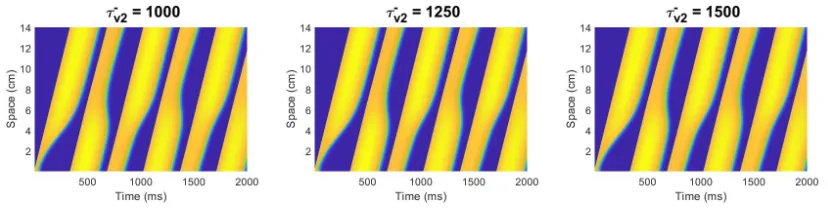
3 Illustration of the dynamical differences obtained by varying the value ofτv−2by 250
ms. . . 19
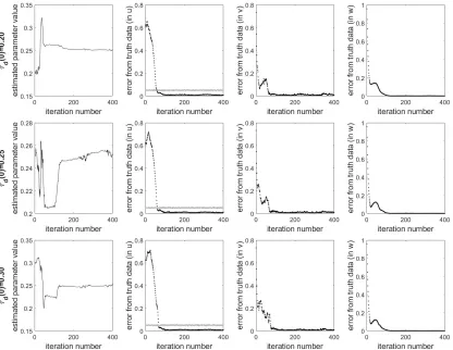
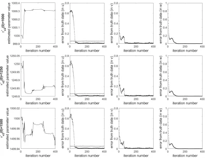
4 Illustration of the inability to estimate τv−2 regardless of initial guess. Each row
corresponds to the estimation ofτv−2given a different initial guess of τv−2(0). The
leftmost plot in each row shows the estimation ofτv−2, and the right three plots show
the RMSE of the state estimation of the 3 model variables, with a gray observation
line present in theufigure for reference. . . 20
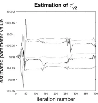
5 Illustration of the inherent randomness of the parameter estimation algorithm.
Each line represents a different attempt at estimating τv−2 from the same initial
conditions. The differences can be explained by pseudo-random numbers being
used throughout the algorithm, including the generation of the initial ensemble
members and the observational data. The true value ofτv−2is 1250, and the mean
and standard deviation of the estimated value of the parameter is 1000.015±0.041. 22
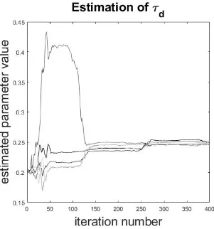
6 Illustration of the success of parameter estimation ofτdregardless of randomness
used in the algorithm. Each line represents a different attempt at estimatingτdfrom
the same initial conditions. All cases converge to the true value of 0.25, although
the randomness affects both the convergence speed and the transient behavior of
the parameter estimation before it reaches the true value. The mean and standard
deviation of the estimated value of the parameter is 0.249±0.003. . . 23
7 Illustration of the success of parameter estimation of certain parameters to which the
model is dynamically sensitive. In the second panel,τr does not reach its true value,
but it does get within a range where the dynamical differences are indistinguishable
by eye. The other three cases show the parameter estimation converges to the true
8 Illustration of the dynamical differences obtained by varyinguv. . . 25
9 Illustration of the inability to estimate uv reliably, as predicted. The multiple
lines correspond to different attempts to estimate the parameter, but vary due to
randomness in the algorithm. The true value of uv is 0.04, and the mean and
standard deviation of the estimated value of the parameter is 0.145±0.133. . . 26
10 Illustration of the dynamical differences obtained by varyingk. . . 28
11 Illustration of the inability to estimatek. The multiple lines correspond to different
attempts to estimate the parameter, but vary due to randomness in the algorithm.
The mean and standard deviation of the estimated value of the parameter is 7.989±
0.136. . . 29
12 Illustration of the estimation ofτdwith different multiplicative inflation values. Each
line represents a different attempt at estimatingτdfrom the same initial conditions.
The true value ofτdis 0.25. The resulting estimated parameter values’s mean and
standard deviation are: 0.225±0.007, 0.249±0.003, and 0.252±0.005, respectively.
The multiplicative inflation factor of 1.7 provided the best results, both in closest
mean value, and smallest standard deviation. . . 31
13 Illustration of the estimation ofucwith different multiplicative inflation amounts.
Each line represents a different attempt at estimating uc from the same initial
conditions. The true value ofucis 0.13. The resulting estimated parameter values’s
mean and standard deviation are: 0.118±0.007, 0.130±0.002, and 0.129±0.003,
respectively. . . 33
14 Illustration of the estimation ofτv−2with different multiplicative inflation amounts.
Each line represents a different attempt at estimating τv−2 from the same initial
conditions. The true value of τv−2 is 1250. The resulting estimated parameter
values’s mean and standard deviation are: 999.996±0.005, 1000.015±0.041, and
999.983±0.157, respectively. . . 34
15 Illustration of the estimation ofτv−2with a multiplicative inflation value of 2.2. This
shows the inability to estimate the parameter even when exceeding our initial
multiplicative inflation maximum. The true value of τv−2 is 1250. The mean and
standard deviation of the estimated value of the parameter is 999.228±0.688. . . . 35
16 Illustration of the system dynamics whenτdandusic have relative errors of 20% and
17 Illustration of the successful estimation ofτdandusic simultaneously. The Fenton-Karma
model has been shown to be sensitive to both parameters and both parameters are
reliably estimated simultaneously. The true values ofτdandusic are 0.25 and 0.85,
respectively. . . 37
18 Illustration of the system dynamics whenτdandτv−2have relative errors of 20% and
remain uncorrected. The true values ofτdandτv−2are 0.25 and 1250, respectively. . 38
19 Illustration of the estimation of τdandτv−2simultaneously. The parameter to which
the model is sensitive,τd, is estimated well, and the parameter to which the model
is not sensitive,τv−2, is not estimated well. Both of these parameters were estimated
simultaneously, but are displayed on separate plots due to their difference in scale.
The true values ofτdandτv−2are 0.25 and 1250, respectively. . . 39
20 Illustration of the system dynamics whenτv−2anduvhave relative errors of 20% and
remain uncorrected. The true values ofτv−2anduvare 1250 and 0.04, respectively. . 40
21 Illustration of the estimation ofτv−2anduvsimultaneously. The Fenton-Karma model
is insensitive to both of these parameters, and they were unable to be estimated
separately. The parameters were estimated simultaneously but are displayed on
separate plots due to their difference in scale. The true values ofτv−2anduvare 1250
and 0.04, respectively. . . 40
22 Illustration of the estimation ofτdandusic simultaneously. Both of these parameters
have been shown to be sensitive in the model. The true values ofτdandusic are 0.25
C
ontents
I Introduction 1
II Methods 4
II.1 Overview of the Fenton-Karma Cardiac Model . . . 4
II.1.1 History and Definition . . . 4
II.1.2 Numerical Implementation . . . 6
II.2 Overview of Kalman Filters . . . 7
II.3 The Local Ensemble Transform Kalman Filter . . . 7
II.3.1 Mathematical Formulation . . . 7
II.3.2 Initialization of the Ensemble . . . 11
II.3.3 Ensemble Undersampling . . . 12
III Parameter Estimation 14 III.1 Introduction . . . 14
III.2 Methods . . . 15
III.3 Estimation of One Spatially and Temporally Homogeneous Parameter . . . 16
III.3.1 Effect of Parameter Dynamics . . . 16
III.3.2 Effect of Parameter Magnitude . . . 25
III.3.3 Effect of Multiplicative Inflation . . . 30
III.4 Simultaneous Estimation of Two Parameters . . . 36
IV Conclusion 43 IV.1 Results . . . 43
IV.2 Limitations . . . 46
IV.3 Future Work . . . 47
I.
I
ntroduction
In the United States, cardiovascular disease is the leading cause of death, claiming the lives of
over 801, 000 people in 2017, accounting for almost one third of all deaths in the country [5]. Heart
disease has also been steadily increasing in prevalence over the past decade, causing it to be an
ever-increasing threat. Despite advancements in the care and prevention of heart disease, 23.6
million people in the world are expected to die annually from heart disease by 2030 [5]. Cardiac
events are often difficult to predict due to their often asymptomatic nature; the person often shows
no symptoms until suffering the cardiac event itself, which can prove fatal. These cardiovascular
complications can occur when the electrical signals propagating throughout the heart become
unorganized or chaotic, resulting in irregular heart contractions, or arrhythmias.
Cardiac arrhythmias are irregular beatings of the heart, such as tachycardia (an abnormally fast
heart rate) or bradycardia (an abnormally slow heart rate). Arrhythmias are often the precursors
to more serious cardiac complications, such as heart failure, stroke, or cardiac arrest [2].
There has been strong evidence to suggest that potentially lethal arrhythmias could be caused by
deformations or instabilities in the cardiac action potential [6, 17], which is a physical occurrence
in a cell in which the membrane potential spikes in a process called depolarization, followed by a
return to a resting potential in a process called repolarization. This entire process of depolarization
and repolarization happens on the time scale of a few hundred milliseconds. These cardiac cells
are excitable media, and as such they have a threshold for excitation and an associated refractory
period to allow time between excitations in a single cell.
Due to the biological knowledge that the electrical signals propagating throughout the heart act as
the coordinator of the heart, telling it to beat together and evenly, it is important to understand
exactly how the electrical impulses travel throughout the heart. In a laboratory setting, an electrode
mesh can be placed about the surface of the heart in order to take recordings of the electrical
potential at each electrode. However, this approach poses two problems: the spatial and temporal
resolution limitations constrain how good of a "snapshot" we get of the surface of the heart at
a given time, and there are no measurements of the electrical potential in the interior of the
heart.
The process of using voltage-sensitive dyes to measure the membrane potential of the heart is the
more modern approach to making experimental data about the voltage across the surface of the
mapping technology, but it does not provide a complete snapshot, as data is subject to noise [12].
Voltage-sensitive dyes have mostly been limited to the surface, and close to the surface of the heart,
leaving much of the interior of the heart unobservable. As such, we do not have a precise method
to take exact measurements of the voltage in the interior of the heart in the same way that we do
about the surface of the heart. This lack of data makes prediction of cardiac events even more
difficult, as the surface voltage may look healthy, but the interior voltage may be becoming chaotic
or otherwise disorganized, which can lead to fatal cardiac events. There have been experiments
that have shown the interior and exterior surfaces of the heart to have very dissimilar dynamics,
which indicates the potential complex intramural dynamics occurring in the heart and solidifies
the needs for more information about the interior of the heart in order to gain a complete picture
of the dynamics occurring in the heart [10].
The lack of complete observational information about the system leads to a problem of attempting
to estimate the entire state of the heart given sparse and noisy data (due to the constraints of the
method of experimental observation, whether it is an electrode mesh or a more modern method
such as optical mapping [3]). The problem of state estimation has in general been solved using a
Kalman Filter, with well-known examples coming from the fields of weather forecasting and signal
processing. In the context of cardiac modeling, we will be using a specific nonlinear extension of
the Kalman Filter, the Local Ensemble Transform Kalman Filter (LETKF) [15], to solve the state
estimation problem. This has shown to be a good method of performing the state estimation in
the cardiac model we will be using, the Fenton-Karma model [14, 20].
In this thesis, we extend the usage of the LETKF by simultaneously estimating the state of
the system and estimating a set of parameters of the Fenton-Karma model. The goal of the
simultaneous estimation of both the state and the parameters is to reconstruct the state of the
system given only sparse, noisy data and to recover the values of the parameters associated with
the true state of the system. We will estimate a single model that is spatially and temporally
homogeneous (unchanging across the time of estimation and having a uniform value throughout
the entire system). From the estimation of a single parameter, we will analyze patterns in the
estimation of the parameter to determine the factors that influence the success of the algorithm,
thereby allowing us to predict whether a parameter is likely to be estimated well and if there
are any methods to improve the chance of successful estimation. We will then estimate multiple
parameters simultaneously in conjunction with the state of the system and show that the same
rules govern the success of the algorithm when estimating multiple parameters as they do when
at the case of the estimation of a single parameter, and to have reasonable assurance that the same
results apply when estimating multiple parameters simultaneously.
The remainder of this thesis is organized as follows. In Section II we provide an overview
of the mathematical model we are using in conjunction with the LETKF and to generate our
synthetic data, including information about the numerical implementation of the model. We
also give an introduction to Kalman Filters and the LETKF specifically, and provide technical
details about the choices made for tuning parameters and initialization methods of the Local
Ensemble Transform Kalman Filter. We also provide a table of common variables used throughout
the thesis for reference. In Section III we show the results of the parameter and state estimation
with subsections to group related results together. Here we illustrate the three factors we have
identified as important for the success of the parameter estimation and we demonstrate that these
results also hold in the case of the simultaneous estimation of multiple parameters. Finally, in
Section IV we conclude our thesis with a discussion of the insights gained into the parameter
estimation problem using our methods and a discussion about future work that could be done to
II.
M
ethods
This section is primarily broken down into two parts: the Fenton-Karma model and the Local
Ensemble Transform Kalman Filter (LETKF). In the first half of this section, we discuss the history
and definition for the Fenton-Karma model, providing information about the motivation for its
application in our project, and providing information about the numerical implementation of said
model. In the second half of this section, we discuss the LETKF and discuss how we incorporate
the Fenton-Karma model in this method of data assimilation to solve the state estimation problem
in cardiac tissue.
II.1
Overview of the Fenton-Karma Cardiac Model
II.1.1 History and Definition
The development of the Fenton-Karma model in 1998 was propelled by the desire to model the
complex electrical dynamics that occur along the ventricular cell membrane in as simple a way as
possible. The goal of the model was to be able to quantitatively reproduce the restitution curves
produced from other complex cardiac models and experimental data by using the least amount of
ionic channel complexity as possible [9].
The model was inspired in part by the earlier Fitzhugh-Nagumo model. This model is a simplified
"caricature" of a general excitable media that can be given the interpretation of a cardiac cell, and
can capture the general behavior of the membrane potential. As a tissue-level representation of
the cardiac dynamics, it is described by the equations
∂tu=∇ ·(D∇u) +3u−u3−v,
∂tv=ε(u−δ),
(1)
whereuis a dimensionless measure of the membrane potential,Dis a diffusion coefficient,vis
representative of the membrane conductance,εis a small parameter that measures the abruptness
of excitation, and δ is a parameter that measures the excitability of the membrane [9]. The
Fitzhugh-Nagumo model continues to be used to study the basic wave behavior of excitable
systems, especially based upon its dependence of the simplified parameter set of{ε,δ}. This
be used as a benchmark against other more complicated models to study the effects of more
complicated parameter sets being introduced into the mathematical models[26].
However, the Fitzhugh-Nagumo model has been shown to be unable to capture the restitution
properties and exact shape of ventricular action potentials [8]. As a result of this shortcoming,
subsequent Fitzhugh-Nagumo-inspired models have added complexity in order to be able to
capture more realistic dynamics which have been observed experimentally [18]. Other models,
such as the 1977 Beeler-Reuter model, applied new-found knowledge of the calcium channel in
ventricular cells to make a ventricular cell-specific model in the spirit of the Hodgkin-Huxley
model [13], in contrast to a generic excitable media model, as was the case in the Fitzhugh-Nagumo
model [4].
The Fenton-Karma model [9] attempts to capture more domain-specific knowledge of cardiac cells,
such as the ion channels that contribute to the transmission of voltage flowing through the cell
membrane. In doing this, the Fenton-Karma model makes the following simplification:
Iion =If i(V;v) +Iso(V) +Isi(V;w), (2)
where Iion is the total current flowing through the cell membrane,If iis the fast inward current
responsible for depolarization of the membrane, Isois a slow outward current responsible for
the re-polarization of the cell membrane, andIsiis a slow inward current which helps to balance
Isoduring the plateau phase of the action potential [9]. The currentsIf i,Iso, and Isi correspond
to the sodium, potassium, and calcium currents, respectively. This is an oversimplification, as
other studies have shown the electrical dynamics across the membrane are much more complex
than can be captured by three individual currents [22]. Nevertheless, the minimal ionic channel
complexity present in the Fenton-Karma model has still proven able to capture many complex
cardiac dynamics, including the ability to generate alternans and recreate restitution curves
observed experimentally.
The purpose of the Fenton-Karma model is to only keep the minimal ionic complexity in order to
capture the restitution properties of the cardiac cells. As such, this model is unable to represent
specific measurements of the trans-membrane currents and cannot claim to have a complete
snapshot of the underlying biological mechanisms of the currents. However, this model is able to
capture the restitution properties of the ventricular cells quantitatively. As such, the parameters
guiding the Fenton-Karma model can be found by curve-fitting of the experimentally-observed
With this simplification of ionic current, the Fenton-Karma model can be described by the
equations
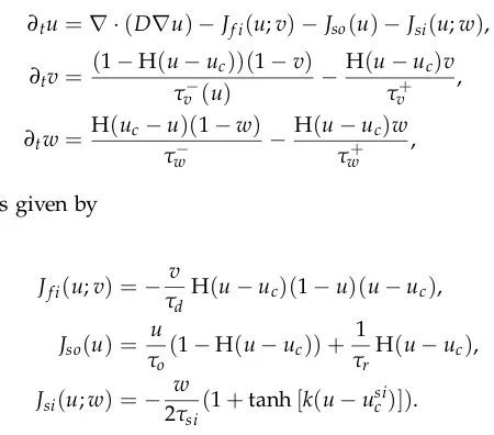
∂tu=∇ ·(D∇u)−Jf i(u;v)−Jso(u)−Jsi(u;w),
∂tv= (1−H(u−uc))(1−v) τv−(u)
−H(u−uc)v τv+
,
∂tw= H(uc−u)(1−w) τw−
−H(u−uc)w τw+
,
(3)
with the three currents given by
Jf i(u;v) =− v
τd
H(u−uc)(1−u)(u−uc),
Jso(u) = u τo
(1−H(u−uc)) + 1 τrH
(u−uc),
Jsi(u;w) =− w
2τsi
(1+tanh[k(u−usic)]).
(4)
In these equations, H(x)denotes the standard Heaviside step function defined by
H(x) =
0 x<0
1 x≥0
. (5)
The variableurepresents a dimensionless membrane potential, and both variablesvandware gate
variables responsible for the inactivation and reactivation ofIf iandIsirespectively. The various
other parameters of the model consist of the time constantsτd,τo,τv+,τv−,τw+,τw−; the threshold
potentialsuc,usic; and uv, and the constantk. As previously mentioned, as the Fenton-Karma
model aims to reproduce quantitative features of ventricular action potentials, the parameters are
chosen to fit specific restitution curves in order to give realistic output.
For our purposes, we have selected parameter values that fit the restitution curves of the original
Beeler-Reuter model with standard parameter values [4]. These selected parameter values can be
[image:15.612.189.414.142.340.2]found in the table in the original Fenton-Karma model paper [9] and are provided for reference in
Table 2.
II.1.2 Numerical Implementation
While a main motivating factor of employing the methods discussed in this paper relies upon
of the tissue, we will implement these methods in a one-dimensional setting. This is done due
to the complexity of the problem drastically increasing in higher dimensions and because of the
usefulness of establishing results and interpretations in a one-dimensional setting before moving
to a higher-dimensional setting.
We will be using a standard Forward Euler discretization of the Fenton-Karma model to propagate
the solution forward in time. As such, we will provide an initial condition of the initial profile of
the variablesu,v, andwin the one-dimensional setting. We will use a ring geometry, in which we
have a cable with periodic boundary conditions, in order to allow the generated action potential
to run indefinitely without intervention.
We use a spatial resolution of 0.25 mm and a temporal resolution of 0.05 ms.
II.2
Overview of Kalman Filters
The goal of a Kalman Filter is to produce an improved estimate of a system’s state by combining
observational data with a numerical model’s predictions. Of course, external factors such as noisy
observational data or error in the model can limit the success of the forecasting ability. A Kalman
Filter seeks to combine a mathematical model and observational data together in a way that is
better than either separately, taking into account possible model error or noisy observational input
[16].
For our purposes, we use an extension of the general Kalman Filter, the Local Ensemble Transform
Kalman Filter [15], in order to improve our estimate of the voltage across the membrane in our
one-dimensional ring geometry. We will use the Fenton-Karma model as the numerical prediction
model in the Kalman Filter. For the present study, we will create our own synthetic data (with
some added Gaussian noise) in order to recreate what realistic observational data would be like,
which will allow us to assess the accuracy of our approach due to having access to the true state
of our system for all time points.
II.3
The Local Ensemble Transform Kalman Filter
II.3.1 Mathematical Formulation
We will first begin by describing the mathematical formulation of the Local Transform Kalman
estimation of the membrane potentialuin the Fenton-Karma model.
The LETKF [15] is a particular type of ensemble Kalman Filter which is a nonlinear extension
to the general Kalman Filter. Ensemble Kalman Filters such as the LETKF attempt to minimize
error variance by using a small number of model states to characterize the covariance of the prior
forecast, the estimate of the state of the system including information about observational data
points from the previous timestep. This collection of model states is referred to as the ensemble.
The number of ensemble members is typically small (which is a big factor in why ensemble
Kalman Filters are used in large, complex problems), usually between 10 and 100 [14]. We will
denote the number of ensemble states ask.
The process of the LETKF is largely split into two separate halves: the background and the
analysis. The background can be thought of as the prior forecast of the system derived purely
from the numerical prediction model (in statistics, this would be called the "prior"). The analysis
combines observations with the background state estimate (in statistics, this would be called the
"posterior").
Let{xb(i) :i = 1, 2,· · ·,k}be the background ensemble (the set of allkbackground ensemble
members). Each background memberxb(i)is a model forecast from the previous timestep and
contains information from previous observations (if this is not the first time step with observation
points) and information from the model’s propagation forward in time. We assume that the
background has an unbiased Gaussian error with mean 0 and variance(0.05)2, and we establish
our initial guess of the background state to be the average of the background ensemble,
xb= 1
k k
∑
i=1
xb(i), (6)
and the background covariance is the sample covariance of the ensemble,
Pb= 1
k−1 k
∑
i=1
xb(i)−xb xb(i)−xbT. (7)
With this information, we now have an estimate of the background at the current timestep,xb,
and have successfully parameterized the covariance of the ensemble,Pb. It is at this point that we
transition from the background to the analysis step. In doing this, we introduce theHoperator
which is an operator from the model space to the observation space. If we label the true state of
yo =H(xt) +ε, (8)
whereyo are the observations for the current timestep, andεis the unbiased Gaussian noise we
assume our methods of observation induce. The values for the Gaussian noise of the observations
is chosen from the normal distribution with mean 0 and variance(0.05)2,N(0, 0.052), in order to
approximate the amount of noise induced by using optical mapping techniques. It is worth noting
thatHcould be a nonlinear map, although in this paper, we will use a linear map for H.
We are using the LETKF, which means that we specify a localization "radius" and that the analysis
step for a given point in the model space only includes observational information from points
within that localization radius. This can decrease the computational cost in large models and also
helps reduce erroneous or unwanted correlations of data across large distances [14]. Numerically,
we achieve this in a simplistic method by giving observations within the specified radius a weight
of 1 and a weight of 0 to points outside this radius.
All Kalman Filters, like the LETKF, will then combine these observation points with the background
estimate in such a way that a specific cost function is minimized. From this analysis step, we can
then characterize the analysis covariance in much the same way that we characterized it for the
background covariance. The analysis ensemble is then constructed by adding the perturbations
predicted by the estimated analysis covariance to this analysis estimate. Then, the new analysis
ensemble is used as the initial state in order to propagate the model forward in time. More details
of this process are available in detail in previous papers [15, 7].
From here, the model is run forward in time. The LETKF is an iterative process, and this resulting
analysis ensemble will become the background ensemble in the next iteration step. As such, the
background ensemble at this new timestep will encode previous information about the dynamics
of the model and information about previous observations.
Outside of mathematical formalism, it helps to put this in practical, tangible terms that relate
directly to the application domain of cardiac electrophysiology. We initialize the model by a set of
potential model states — which we will discuss in further detail in section II.3.2 — , and we are
interested in assimilating observations of theuvariable, a measure of the membrane potential
along the tissue. We are interested in seeing how accurately we can estimate the membrane
potential with a non-perfect model, and with noisy observational data. The observational data
points that we use are synthetic, generated by taking the true state of the system (which we obtain
analysis step of assimilation.
From this, we have both the "truth" and the observational data points (as the observational data
points are created by sampling the truth and adding Gaussian noise). The truth will be used to
benchmark against the estimate of the system over time, in order to gauge the accuracy of the
estimation of the state and the parameters over the course of assimilation. Ideally, even if the initial
estimate is poor, the LETKF should be able to reduce error between the truth and the estimate
over time by incorporating observational data which we provide. The goal is that even though the
observational points are noisy, they should — hopefully — be able to provide enough information
over many iteration cycles to guide the estimate back to the true state of the system.
A concrete example of the usefulness of this algorithm could be imagined in the three-dimensional
setting, in which we have a heart and we use optical mapping techniques to make measurements
of the voltage along the surface of the heart. We can make measurements of the membrane
potential at a specified spatial resolution at fixed time intervals, with some observational error
induced from non-perfect sensors. We want to be able to "guess" some possible initial states of the
heart to form the background ensemble and then use the LETKF to incorporate the observational
data. If the LETKF works properly, this means that the ensemble members should converge over
time to a faithful representation of the true system state.
By using a model to generate "truth" data and synthetic observations, we are able to benchmark
how well the LETKF algorithm performs over time. In a laboratory setting, the "true" state of the
system is not known and, as such, it is rather benchmarked by how well it converges to something
that qualitatively and (to some extent) quantitatively captures the future dynamics of the system.
In this sense, the test of accuracy is how well the newfound system estimate can capture the
future behavior of the true system in the future. As we are not working in a laboratory setting
and have access to the true state of the system, we can instead test accuracy directly by checking
convergence of the state estimation to the true state of the system. Since we generate the truth and
observational data, we will be able to measure accuracy at each timestep and to make conclusions
that can be extrapolated to real-world information, where the "true" state of the system is not
known at the outset.
This thesis is based upon the seminal work of data assimilation on cardiac electrical wave dynamics,
and additional explanation of the LETKF process with respect to cardiac electrodynamics can be
found there [14, 20].
thesis.
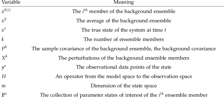
Variable Meaning
xb(i) Theithmember of the background ensemble
xb The average of the background ensemble
xt The true state of the system at timet
k The number of ensemble members
Pb The sample covariance of the background ensemble, the background covariance
Xb The perturbations of the background ensemble members
yo The observational data points of the state
H An operator from the model space to the observation space
m Dimension of the state space
[image:20.612.89.520.119.310.2]Pi The collection of parameter states of interest of theithensemble member
Table 1:Common variables used throughout the thesis.
II.3.2 Initialization of the Ensemble
How the ensemble is initialized can play a vital role in the success of the algorithm. In the previous
section, we stated that we take several "guesses" of what the system may look like - be it from
propagation of a model or information about the application area - and use those as the initial
ensemble members.
In our case, we choose to run the Fenton-Karma model for a "spinup" of 1000ms. We then run
the model for an additional 100 iterations - with each iteration corresponding to 0.05ms - and
then sample ourkinitial ensemble members from these last 100 iterations. This idea behind this
method of initialization was first proposed in the seminal LETKF paper by Hunt et al [15].
Running the model for 1000 ms will allow any transient effects such as sharp wavefronts to settle
down into long-term behavior expected with periodic boundary conditions. For our initial guess
of parameters to generate the ensemble (and the truth data) we use the parameters to match
the restitution curves of the Beeler-Reuter model [4]. We then randomly sample the next 100
iterations to obtain thekensemble members (k=20). Sampling the iterations randomly has been
shown to be a reasonable choice to characterize the initial ensemble and covariance in the weather
forecasting community [15]. This method has also been suggested as a suitable method when no
the ensemble with no observational information available yet.
The creation of the initial ensemble by allowing for a "spinup" and then a random sampling has
been shown to capture the covariance of the initial ensemble sufficiently so as to prevent ensemble
collapse: when the members of the ensemble become too alike, potentially causing estimation
problems and skewing the covariance [21]. While ensemble collapse can still happen after many
iterations of the LETKF, as the ensemble members may gradually converge to a single shape, this
method of selecting initial ensemble members provides enough spread to initially characterize the
system without the possibility of early ensemble collapse.
II.3.3 Ensemble Undersampling
The LETKF performs the analysis step (the combination of the forecast with the observational data
for the current iteration) in ensemble space. That is, the analysis step finds an optimal solution
(minimizes a cost function) that is a linear combination of the ensemble members. This usage of
the ensemble members to estimate the covariance and update the state estimate is a significant
computational savings when the number of ensemble members is less than the dimensionality of
the state space, as it reduces the problem from anm×mproblem into ak×kproblem, wherem
is the dimensionality of the model space andkis the number of ensemble members. In our case,
this is a reduction by two orders of magnitude (a reduction from 103to 101).
However, in cases where the ensemble space is much smaller than the state space — which is most
often the case of ensemble-based Kalman Filters — problems can arise from undersampling. The
LETKF attempts to estimate the covariance of the state by using the sample covariance obtained
from the ensemble members; it also attempts to form the analysis as a linear combination of the
ensemble members. This leads to the problem of undersampling of the ensemble variance and
filter divergence, an underestimation of the forecast error that causes the algorithm to ignore the
observations, making it difficult to regain the spread of the ensemble later [25].
The typical solution to this problem is to artificially inflate the uncertainty. To do this, both
multiplicative and additive inflation methods are applied. Multiplicative inflation applies a scaling
factor to thek×kcovariance matrixPb, artificially increasing the uncertainty in the forecast and
helping to prevent filter divergence. Additive inflation adds a vector of perturbations to each
ensemble member. These vectors correspond to the differences in model states which are 5ms
apart during the spinup portion of the initialization algorithm, and are scaled by a positive scaling
step is performed in ensemble space and additive inflation can increase the span of the ensemble
members, this can open up new possibilities for the estimation of the state.
For the purposes of this document, we use a value ofα=0.05 for additive inflation, building
upon previous results [20]. The magnitude of multiplicative inflation varies and can be found in
III.
P
arameter
E
stimation
III.1
Introduction
In many scenarios, it is desirable to be able to extract information about the parameters that guide
a system. This information can be used to gain insight into the future behavior of the system or
to explain retroactively why particular effects occurred. We will attempt to extract the value of
a given parameter in the Fenton-Karma model by using the LETKF algorithm and our "truth"
data.
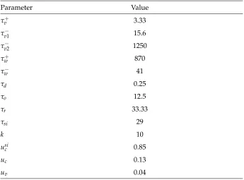
We use a ring size of 135 mm, which corresponds to 540 grid points in our discretized model
(with a spatial resolution of 0.25 mm). Table 2 provides a list of the parameter values used to
generate the truth state of the system from the Fenton-Karma model. These parameter values were
chosen to match the Beeler-Reuter parameter set [9]. This selection of parameter values produces
alternans — an alternation between long and short action potential durations — and exhibits
a stable action potential which will propagate around the one-dimensional ring without being
annihilated.
Parameter Value
τv+ 3.33
τv−1 15.6
τv−2 1250
τw+ 870
τw− 41
τd 0.25
τo 12.5
τr 33.33
τsi 29
k 10
usi
c 0.85
uc 0.13
[image:23.612.134.479.388.643.2]uv 0.04
III.2
Methods
To implement parameter estimation in the LETKF, we will use state-augmentation methods
proposed previously [24, 1]. To estimatepparameter states usingkensemble members, we append
the parameter states to the background ensemble states, producing an augmented set of ensemble
states. If we letP be the collection of parameter states we wish to estimate, the augmented ensemble takes on the following form:
{(xb(i),Pb(i)),i=1, 2,· · ·,k}, (9)
wherexb(i)is theithmember of the background ensemble andPb(i)is the set of parameter states (values) being estimated of the background ensemble memberi. In this case, we have that the
dimensionality ofxb(i)ismand the dimensionality ofPb(i)isp, making(xb(i),pb(i))∈Rm+p.
In the method of parameter estimation we are using, the original background ensemble is
run through the LETKF algorithm as was previously described to produce the corresponding
analysis ensemble. Then we update the parameters in a separate step, obtained from running the
non-localized LETKF, the ETKF, on the augmented background ensemble produced previously.
Using localization has been shown to provide little increase in the effectiveness of reducing
parameter estimation error, so it is common to use the non-localized ETKF in order to reduce the
amount of computation necessary [24, 19]. As such, the parameter estimation step is done without
localization, but the rest of the forecasting of the state and propagation of the ensemble members
forward in time is done using localization, as this can improve the successfulness of the estimation
of the state of the system [15, 11].
After the estimated values of the parameters are updated after being run through the ETKF, they
are inserted into the model for propagation forward in time. From this, the background ensemble
in this next iteration is generated and encodes information about the selection of parameter values.
The covariance matrix now includes information about the successfulness of the estimation of the
parameters, as it was used to propagate the model forward in time, and the results can be directly
compared with the true state of the system,xt. As such, incorrect perturbations (assuming they
are large enough to be non-trivial errors) will be reflected in the covariance, and the algorithm
will attempt to vary the parameter more, in a search for the true value of the parameter.
The purpose of running the LETKF on the original background ensemble, and then the ETKF
background covariance obtained from propagating forward the model in time, and also because
localization can increase the effectiveness of forecasting. This allows the parameter update step
to have more information on which to base the updated parameter values. This background
covariance acts as an indicator of the "closeness" of the estimated parameter value to the true
parameter value. If the state estimation is diverging from the truth, the estimation uncertainty
will be reflected in the covariance matrix, and the algorithm will increase the amount it varies the
parameter (and the analysis ensemble members as a whole) to compensate for uncertainty in its
estimation of the state.
III.3
Estimation of One Spatially and Temporally Homogeneous Parameter
First we attempt to estimate a single parameter that is spatially and temporally homogeneous.
Due to this, we have thatPb(i)∈R, since it is a single value for the parameter for each ensemble member. We simply append this value to our background ensemble members,xb(i), and run it
through the process as previously described.
III.3.1 Effect of Parameter Dynamics
In this section we explore why this method of parameter estimation works better for some
parameter choices than others, with our primary motivation being the system dynamics associated
with the parameter’s value. The next section will address the same underlying question by looking
at the relative magnitudes of the parameter being estimated. The hypothesis is that the more
sensitive the dynamics of the model are to changes in the parameter being estimated, the more
likely the algorithm is to estimate the parameter successfully.
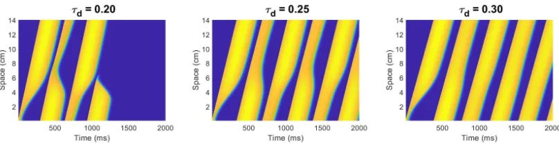
First we consider the estimation ofτd, a parameter that appears in the fast inward current of the
Fenton-Karma model. In Figure 1, we illustrate the dynamical differences caused by varying the
Figure 1:Illustration of the dynamical differences obtained by varying the value ofτdby 0.05 ms−1.
It can be seen from Figure 1 that changing the value ofτdby 0.05 ms (a relative change of 20%)
results in significant differences in the dynamics of the action potential propagating around the
ring; including changes in the speed and wavelength alternation magnitude. With a reduction of
0.05 ms, the wave actually dies off before the simulation of 2000ms finishes. This is due to the fast
inward current being increased whenτdis decreased, causing the wave speed to increase, and
stay excited for longer, causing the wave to collide with itself. This collision of the wave front with
the wave back causes destructive interference, and causes the action potential to be annihilated.
In the case of an increase of 0.05, the action potential stabilizes, removing any alternans in the
wave shape. This can be seen in Figure 1, where the action potential no longer has any oscillations
in wavelength whenτd=0.30. This increase in the value ofτdstabilizes the action potential by
creating system dynamics in which the wave speed is slow enough and the wave dies off quickly
enough to prevent any collisions of the wave front and the wave back.
For the purposes of this section, we will be using a multiplicative inflation value of 1.7 for the
simulation and leave the discussion of the impact of the choice of multiplicative inflation to section
III.3.3. The value of 1.7 for multiplicative inflation is an effective choice for the majority of cases,
based on our numerical experiments. We also use 180 observational points, spaced uniformly
throughout the ring, which is equivalent to using one of every three grid points observable for
usage with the LETKF algorithm.
Figure 2 shows the results of the estimation ofτdwhen the initial "guess" of the parameter to be
estimated is varied. The initial value ofτdis labeled on the left of each row asτd(0). The leftmost
plot in each row shows the estimation of the parameter over the course of assimilation. The three
other plots in each row show the root mean squared error (RMSE) of the state estimation in each of
the three state variables,u,v, andw. The gray line is provided as a reference point, and represents
the amount of observational error at each assimilation step. The value is held around 0.05 due to
for our purposes, we only take observational data about the value ofu, and we do not observev
[image:27.612.103.519.135.457.2]orwfor usage in the LETKF algorithm.
Figure 2:Illustration of the success of the estimation ofτdregardless of initial guess. Each row corresponds
to the estimation ofτdgiven a different initial guess ofτd(0). The leftmost plot in each row shows
the estimation ofτd, and the right three plots show the RMSE of the state estimation of the 3 model
variables (u,v,w), with a gray observation line present in theufigure for reference. Each iteration corresponds to 5 ms.
Figure 2 shows the successful estimation ofτdregardless of whether the initial estimate ofτdwas
over- or underestimated. The error plots provided in all three cases also show the convergence
of the estimation of the system state to the truth, as is desired of any Kalman Filter. As part of
the way that this method of parameter estimation works, the estimated value ofτd is put into
the model in the analysis step, so it is used to create the background in this next iteration by
propagating the model forward in time.
dynamical differences obtained by varying the parameter by 250 ms (a relative change of
[image:28.612.98.512.135.239.2]20%).
Figure 3:Illustration of the dynamical differences obtained by varying the value ofτv−2by 250 ms.
The dynamical differences in the change of this parameter are much more subtle. Despite using the
same relative change in the parameter as forτd, the model is much less sensitive to this parameter,
and as a result the resulting waves look identical to the unaided eye. Figure 4 illustrates the results
Figure 4:Illustration of the inability to estimateτv−2regardless of initial guess. Each row corresponds to the
estimation ofτv−2given a different initial guess ofτv−2(0). The leftmost plot in each row shows the
estimation ofτv−2, and the right three plots show the RMSE of the state estimation of the 3 model
variables, with a gray observation line present in theufigure for reference.
It can be seen in Figure 4 thatτv−2was not estimated well in the cases where the initial selection of
the parameter value was not correct. In all three cases, the parameter changed by a maximum
of 0.3 ms, making it unable to recover the correct value of the parameter over the course of
assimilation.
The explanation for this is the insensitivity of the model to the parameter. As was shown in Figure
3, a change of 250 ms is not visible in the dynamics of the action potentials, meaning that 0.3 ms is
even less noticeable. The LETKF bases its estimates of the covariance on how closely the ensemble
of model states estimates the true state of the system at the current timestep. However, since the
tiny perturbations of the parameter do not produce any noticeable differences in the dynamics
given to it and instead corrects the state estimation through the traditional LETKF process — with
observational data guiding its trajectory over many iterations. As such, when tiny perturbations
of the parameters do not reflect noticeable differences in the model propagation, the LETKF
parameter estimation process fails to move the parameter much, causing its final estimated value
to be approximately equal to the initial value given to the parameter, meaning that it was not
estimated well.
It is worth noting that there are several steps in the algorithm in which stochasticity may impact
the performance of the LETKF and parameter estimation; the randomness in the algorithm may
be created in such a way that the algorithm is able to recover the true value of the parameter(s)
being estimated even if the errors in the estimated value of the parameter(s) does not produce
noticeable affects in the dynamics of the system. In the algorithm, we have randomness inherent
in the selection of the initial ensemble members, the selection of additive inflation values, and the
construction of observational data points. As such, despite having the same setup, different results
may occur for both the effectiveness of the state estimation via the LETKF and the parameter
Figure 5:Illustration of the inherent randomness of the parameter estimation algorithm. Each line represents a different attempt at estimatingτv−2from the same initial conditions. The differences can be explained
by pseudo-random numbers being used throughout the algorithm, including the generation of the initial ensemble members and the observational data. The true value ofτv−2is 1250, and the mean
and standard deviation of the estimated value of the parameter is 1000.015±0.041.
Due to the randomness present in our implementation of the algorithm, the results of both the
state estimation and the parameter estimation are not deterministic. Normally, the results are very
similar and differ by very little, as was the case in Figure 5. However, there are anomalous cases
in which a parameter may be estimated much better in one simulation than another. We have run
every simulation presented in this thesis several times and have selected cases that are largely
representative of the general behavior of the algorithm. For example, there may be an anomalous
case for the estimation ofτv−2in which the algorithm successfully recovers the parameter value
from the same start conditions as present in Figure 5. However, we would not use this case as an
It can be shown that parameters that affect dynamical changes over the time scale of assimilation
are much more likely to be well estimated with the algorithm and will reliably recreate the actual
value of the parameter, even in the presence of randomness in the algorithm. This can be seen
in Figure 6, where we show the algorithm’s ability to determine the true value ofτd, despite the
[image:32.612.162.463.187.509.2]randomness.
Figure 6:Illustration of the success of parameter estimation ofτd regardless of randomness used in the
algorithm. Each line represents a different attempt at estimatingτdfrom the same initial conditions.
All cases converge to the true value of 0.25, although the randomness affects both the convergence speed and the transient behavior of the parameter estimation before it reaches the true value. The mean and standard deviation of the estimated value of the parameter is 0.249±0.003.
From the viewpoint of dynamics, the variables that produce the largest dynamical differences
over the time scale of assimilation seem to be the most reliably estimated. In these cases, the error
induced by incorrect estimation of a parameter at each step is much larger than for a parameter
to more readily add perturbations to the parameter value in an attempt to nudge it towards
the correct parameter value. These apparent dynamical differences caused by the difference in
parameter value cause the ensemble members to have a larger spread, as they all contain slightly
different parameter values. This means that the perturbation matrixXbhas larger entries, since the
ensemble members have greater variance from the mean.This causes the parameter to be estimated
more reliably, as the error is more noticeable in theXbperturbation matrix.
It is also worth noting that the wavefront of the action potential seems to be the strongest indicator
of parameter estimation success. The model seems to be most sensitive to parameters whose value
will affect the wavefront whether that be shape, speed, location, or any other dynamical effect
-and will be reliably estimated via this method. In the example of the estimation ofτdfrom Figure
1,τdmay not appear to affect the wave front, but rather the propensity for alternans and the speed
of the wave. However, the wave speed will impact the location of the wavefront along the ring,
or perhaps even cause the wave to collide with itself and be annihilated. This is an important
part of the state to estimate for the LETKF, and so the impact of the parameter on the position
of the wavefront causes the algorithm to reliably estimateτd, regardless of initial error in the
guess.
We end this section by providing the results of the estimation of 4 sensitive parameters of the
Fenton-Karma model, with initial values starting 20% below their true value. As they have
strong effects on wave fronts in the model, the parameter estimation algorithm does a good job at
recovering the true value of the parameters throughout the assimilation process. The results are
[image:33.612.95.518.487.595.2]displayed in Figure 7.
Figure 7:Illustration of the success of parameter estimation of certain parameters to which the model is dynamically sensitive. In the second panel,τrdoes not reach its true value, but it does get within a
This is further evidence that the dynamics induced by error in the parameter values strongly
impacts the success of the parameter estimation algorithm. It also shows that these sensitive
parameters can be reliably estimated, despite randomness inherent at multiple stages in each run
of the algorithm.
III.3.2 Effect of Parameter Magnitude
In this section we further explore why this method of parameter estimation works better on some
parameter choices than others, with the primary motivation being the importance of the magnitude
of the parameter we are estimating. We also show experimental evidence that parameters are
more likely to make larger relative changes of their values over the course of assimilation if their
magnitudes are small in comparison to the rest of the parameters of the model. The explanation
behind this phenomenon is that for large parameter values, the perturbations that get added
during the algorithm are simply not large enough to notice bigger errors in the parameters. If the
parameter is small, the perturbations added are relatively bigger, which means that the parameter
estimation algorithm is more likely to change the value of the parameter significantly during the
estimation process, in contrast to remaining stagnant, as is the case with many large, insensitive
parameters, such as in Figure 5. These larger perturbations in the parameter estimation may
increase the likelihood that the algorithm estimates the parameter successfully.
We first look at the case of a small parameter,uv. The true value foruvin the truth data is 0.04 (all
variable values for truth data are provided in Table 2). We estimate from 0.32, a relative error in
[image:34.612.98.514.514.620.2]the parameter of 20%. We provide the dynamical differences incurred by incorrect values ofuvin
Figure 8.
Figure 8:Illustration of the dynamical differences obtained by varyinguv.
Figure 8 illustrates that the dynamical differences caused by varyinguvare indistinguishable to
we can likely guess that this parameter will not be estimated well. We provide the results of the
[image:35.612.145.463.129.458.2]estimation ofuvin Figure 9.
Figure 9:Illustration of the inability to estimateuvreliably, as predicted. The multiple lines correspond to
different attempts to estimate the parameter, but vary due to randomness in the algorithm. The true value ofuvis 0.04, and the mean and standard deviation of the estimated value of the parameter is
0.145±0.133.
From Figure 9, we can deduce thatuvis not reliably estimated via the ETKF algorithm, as it only
recovered the true value of the parameter in one run out of five attempts. However, the initial start
point for the parameter was 0.032, and the parameter decreased by 0.032, and increased by 0.298, in
some simulations. These correspond to relative differences of 100% and 931%, respectively.
In the estimation of large parameters using this method, the algorithm is much more likely to
remain stagnant if there are not large dynamical differences - a phenomenon explored in the
previous section. However, in the case of smaller parameters, such asuv, the algorithm is more
This is due to the perturbations applied during the algorithm being large relative to the parameter
value itself.
This can be seen by contrasting Figures 9 and 5. In Figure 5,τv−2is being estimated from an initial
value of 1000, but over the course of estimation, its value only changes by a maximum of .15, a
relative change of 0.015%, despite the true value of the parameter being 1250. However, in Figure
9, as was previously mentioned, we obtain a much larger relative and absolute change in the value
of the parameter.
Our hypothesis is that parameters with smaller magnitudes will in general be more prone
to move larger distances from the initial value of the parameter, in an effort to find the true
value of the parameter. The reasoning behind this hypothesis is that the algorithm is applying
random perturbations to the parameter being estimated, and the ensemble. However, these
perturbations are held at the same size, regardless of parameter being estimated. This means
that the perturbations applied when estimating smaller parameters are relatively much larger
than the parameters themselves, which in turn makes the error in the estimated parameter be
overestimated during the algorithm. This overestimation then leads the algorithm to "self-correct"
itself by varying the parameter value by relatively larger amounts in an effort to decrease the
overestimated error in the parameter estimation.
These larger changes in the parameter, of course, die down after the state estimation problem has
been solved by the LETKF. That is, the parameter changes will decrease in magnitude once the
RMSE of the state estimation in all 3 variables has converged to low error. This does not mean that
the error is no longer being overestimated or that the parameter has reached the correct value. This
simply means that the state is being estimated sufficiently well, so that the Kalman Filter does not
require changes to the parameter in order to maintain low RMSE in the state estimation problem;
it has achieved a low enough RMSE where the Kalman Filter can continue to provide a good
estimate of the state using only the numerical prediction model and the provided observational
data.
We next look at another variable used in the Fenton-Karma model: k. This variable appears in
the formulation of the slow inward current,Jsi. The true value of this parameter is 10, and we
estimate it from the value of 7.5. The dynamical differences caused by varying the parameterk
Figure 10: Illustration of the dynamical differences obtained by varyingk.
Figure 10 shows that increasingkfrom 10 to 12 does not produce large effects in the dynamics
of the wave on a macroscopic level. However, decreasing the value from 10 to 8 - as we shall do
when estimating the parameter in the next figure - does produce noticeable dynamical differences.
In particular, the waves tend to stabilize, removing almost all oscillations in the wavelength from
the resulting space-time diagram. This removal of oscillations in the space-time diagram simply
corresponds to the wave reaching a more stable position, removing most of the alternans. The
results of parameter estimation from an initial value of 8 are shown in Figure 11. The inability
of the algorithm to recover the true value ofkis perhaps unexpected, as visible differences in
the dynamics of the action potentials are present in the diagrams. The error in the value of this
parameter is responsible for having an incorrect wavelength and much less pronounced alternans.
However, the lack of larger differences in the morphology of the wave - in particular, differences
in the wave front - prevents the algorithm from having pronounced error in the state estimation.
Errors in the wavelength - when not severe - are too similar to the observations when the rest
of the ring is being estimated well. Due to the overall good estimation of the state (outside of
locations where the wavelength is off), the parameter will not make large changes, and is not
Figure 11:Illustration of the inability to estimatek. The multiple lines correspond to different attempts to estimate the parameter, but vary due to randomness in the algorithm. The mean and standard deviation of the estimated value of the parameter is 7.989±0.136.
In this case, the parameter is varied by a change of up to 0.3, which is roughly the same change
experienced in Figure 9. It can be seen that the final estimated parameter values often varies
heavily from simulation to simulation, as was the case in Figure 9. This is the crux of the
importance of parameter magnitude: the parameter value impacts how much the perturbations
cause the estimated parameter value to change, which in turn leads to more divergent parameter
estimation results from simulation to simulation. Experimentally, the dependence upon the
magnitude of the parameters leads to more varied results in estimating low parameters and makes
analysis of the effectiveness of the parameter estimation difficult, as any successful parameter
estimation may simply be due to the randomness in the algorithm, much more than estimating
larger parameters.
regarding the effectiveness of the parameter estimation. Small parameters to which the Fenton-Karma
model is sensitive have been shown to converge to approximately the same value regardless of
randomness. This can be seen in Figure 7, where the small parameters τd,uc, and usic are all
reliably approximated despite having magnitudes less than one. However, also in Figure 7, we see
thatτr is pretty reliably estimated as well, as the model is moderately sensitive to the parameter.
However, it is an order of magnitude larger than the other parameters in the figure, and we see the
most variability in the results of its estimation. This variability can be accounted for in part by the
magnitude being larger, and thus when it approaches the true parameter value, its perturbations
grow relatively very small, and as such the algorithm will not correct the parameter value further,
leaving the parameter value to remain unaffected. The magnitude of the parameter prevents it
from fine-tuning to the exact value of the parameter; accuracy is achieved for the LETKF state
estimation problem without obtaining a good parameter estimation.
III.3.3 Effect of Multiplicative Inflation
Multiplicative inflation is used to mitigate underestimation of the variance of the ensemble,
which results from ensemble undersampling (using too few ensemble members when working
with high-dimensional states) [25]. In the context of parameter estimation, this multiplicative
inflation is applied to the augmented ensemble containing the parameter state(s) being estimated.
In this manner, the augmented ensemble perturbation matrixXb is inflated, meaning that the
perturbations of the parameter(s) are increased. These additional perturbations serve to decrease
the confidence of the ETKF in the selection of the parameter, as there is more variance of the
parameter, thus making the algorithm more apt to change the value of the parameter over the
course of estimation.
As such, the multiplicative inflation factor to be used is an important parameter in and of itself that
can affect the successfulness of the parameter estimation. Throughout sections III.3.1 and III.3.2,
we have been using a fixed value of 1.7 for multiplicative inflation, as this has been shown to be a
generally good selection of inflation value. However, in this section, we will explore the impact
that the multiplicative inflation value can have on the performance of both the state estimation
problem of the LETKF and the parameter estimation of the ETKF.
First, we run simulations for the estimation ofτd, as was done in Figure 6 with an inflation value
of 1.7. We will now estimate the same parameter set with all of the same initial conditions, but
and 2 (corresponding to no inflation and doubling inflation, respectively), so these are good values
to test the lower and upper limits of the inflation value. It is worth noting that a multiplicative
inflation factor of 2 is not a bound on the value, but numerical problems have occurred in our
particular model when increasing the value of multiplicative inflation past 2. The results are
[image:40.612.96.517.192.331.2]provided in Figure 12.
Figure 12:Illustration of the estimation of τd with different multiplicative inflation values. Each line
represents a different attempt at estimatingτdfrom the same initial conditions. The true value ofτd
is 0.25. The resulting estimated parameter values’s mean and standard deviation are: 0.225±0.007, 0.249±0.003, and 0.252±0.005, respectively. The multiplicative inflation factor of 1.7 provided the best results, both in closest mean value, and smallest standard deviation.
Figures 1 and 2 have already shown that the Fenton-Karma model is sensitive toτd. As such,
based on section III.3.1, we would expect the parameter to be generally well estimated, regardless
of randomness used throughout the algorithm in a given simulation.
Figure 12 demonstrates that the choice of multiplicative inflation can greatly influence the success
of the estimation of parameters, even in the case where the model is sensitive to the parameters.
In the case of a lower multiplicative inflation value of 1.2, we see that the parameter estimation
does indeed correct towards the true value of 0.25, but it does not reach the true value over the
assimilation interval of 400 iterations. This matches expectations: due to the lower multiplicative
inflation factor, the variance in the parameter estimation is lower, so the algorithm tends to make
smaller changes to the parameter value between iterations. The smaller changes to the parameter
value then lead to slower convergence to the true parameter value, as the algorithm will not allow
for larger "jumps" in the parameter value to more quickly reach the true value.