Application of Decaying Boundary Layer and Switching Function Method Thorough Error Feedback for Sliding Mode Control on Spacecraft’s Attitude

This is a repository copy of

Application of Decaying Boundary Layer and Switching

Function Method Thorough Error Feedback for Sliding Mode Control on Spacecraft’s

Attitude

.

White Rose Research Online URL for this paper:

http://eprints.whiterose.ac.uk/116108/

Version: Accepted Version

Proceedings Paper:

Hassrizal, H.B. and Rossiter, J.A. orcid.org/0000-0002-1336-0633 (2017) Application of

Decaying Boundary Layer and Switching Function Method Thorough Error Feedback for

Sliding Mode Control on Spacecraft’s Attitude. In: 2017 25th Mediterranean Conference on

Control and Automation (MED). 25th Mediterranean Conference on Control and

Automation 2017, 03/07/2017-06/07/2017, Valletta, Malta. Institute of Electrical and

Electronics Engineers , pp. 1250-1256. ISBN 978-1-5090-4533-4

https://doi.org/10.1109/MED.2017.7984289

© 2017 IEEE. Personal use of this material is permitted. Permission from IEEE must be

obtained for all other users, including reprinting/ republishing this material for advertising or

promotional purposes, creating new collective works for resale or redistribution to servers

or lists, or reuse of any copyrighted components of this work in other works.

[email protected] https://eprints.whiterose.ac.uk/ Reuse

Unless indicated otherwise, fulltext items are protected by copyright with all rights reserved. The copyright exception in section 29 of the Copyright, Designs and Patents Act 1988 allows the making of a single copy solely for the purpose of non-commercial research or private study within the limits of fair dealing. The publisher or other rights-holder may allow further reproduction and re-use of this version - refer to the White Rose Research Online record for this item. Where records identify the publisher as the copyright holder, users can verify any specific terms of use on the publisher’s website.

Takedown

If you consider content in White Rose Research Online to be in breach of UK law, please notify us by

Application of Decaying Boundary Layer and Switching Function

Method Thorough Error Feedback for Sliding Mode Control on

Spacecraft’s Attitude

Hassrizal H. B.

and J. A. Rossiter

∗ † _{Department of Automatic Control and Systems Engineering, The University of Sheffield,}

Mappin Street, Sheffield, S1 3JD, UK

∗ _{School of Mechatronic Engineering, Universiti Malaysia Perlis, Malaysia}

Email:∗ [email protected],† [email protected]

Abstract—Effective operation of small spacecraft implies pro-cessors with low cost, energy efficiency and low computational burdens while retaining accurate output tracking. This paper presents the extension of work in [1] on eliminating the chattering for Sliding Mode Control (SMC) using a decaying boundary layer design which is able to achieve these small spacecraft operation needs. The extension is applied on a spacecraft’s attitude control, while orbiting the earth with angular velocity, ω0. In SMC,

chattering is a main drawback as it can cause wear and tear to moving mechanical parts. Earlier work on a decaying boundary layer design was capable of reducing the chattering phenomena for a limited time only and hence this paper proposes a novel decaying boundary layer and switching function to improve the earlier version. The proposed technique is shown to reduce chattering permanently and also retain control output accuracy.

Keywords: small spacecraft, spacecraft’s attitude, SMC, chatter-ing, decaying boundary layer, switching function, control accuracy

I. INTRODUCTION

A spacecraft or satellite is an object that is orbiting larger objects such as the earth. Currently there are more than 1000 operational man-made spacecraft and satellites in orbit around earth [2]. In this paper, the focus is on control strategies to maintain the spacecraft attitude; consequently there will be some discussion of dynamics and kinematics to determine the angular velocity with respect to the earth.

The spacecraft’s attitude can be as important to control as its position. A spacecraft needs a motion control system to position and orientate itself correctly, especially when disturbances and uncertainties occur. The attitude motion of a spacecraft can be described as a set of differential equations [3]. The motion is given by the spacecraft body rotation with respect to different frames of motion. In space, there are disturbances and uncertainties that influence the coordinates of the spacecraft such as the gravitational force of the earth and moon and atmospheric drag in low earth orbits (LEO) [4]. Hence, a robust controller is required to make sure the spacecraft remains at the correct altitude and longitude and at the right time, moreover while producing high control accuracy.

Many control methods have been developed for a space-craft’s attitude. In this paper, Sliding Mode Control (SMC) is

chosen as the basic control method for spacecraft’s attitude control due to its advantages especially for small spacecraft space exploration, such as LunarSat [5]. Specifically, SMC is well-known as a robust controller, it is low complexity, can have low computational burden, low weight and low cost [6] [7]. Methods such as Adaptive Fuzzy Sliding Mode Attitude Control (AFSMC) [8], that is SMC combined with Adaptive Fuzzy rules and require a high computational load because of a complex fuzzy parameter and are not pursued. On the other hand, Minimum Sliding Mode Error Feedback Control (MSMEFC) [9] is an energy efficient, low complexity, low computational load, high control accuracy and robust control method. Moreover, MSMEFC is suitable for realistic disturbances and uncertainties experienced by a spacecraft in space and includes a cost function to offset the disturbances and uncertainties to improve the control performance.

In SMC, the controller input isu(t) =u(t)eq+u(t)nwhere u(t)eq andu(t)n are denoted as equivalent control input and

natural control input (switching function) respectively. u(t)eq

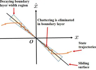
is used to force the state trajectories to move to the sliding surface (si(x) = 0) as in figure 1 (in this time,u(t)n is off).

When the state trajectories hit the sliding surface,u(t)n is on

and ensures the state trajectories move along the sliding sur-face (in this time,u(t)eq is off). Unfortunately, using just the

basis concept of SMC, chattering (figure 1) is a main drawback that can cause wear and tear in the moving mechanical parts. Chattering is produced by the switching function (1) inside the s-plane of the sliding surface (si(x) = 0).

ui(t) =



 

 

u+

i (x, t) withsi(x)>0 0 withsi(x) = 0 u−i (x, t) withsi(x)<0

(1)

Figure 1. Chattering phenomena ons_{-plane in SMC}

spacecraft moved to safe mode because one of the reaction wheels produced unusual readings [10]. It took time before the recovery action was taken and this problem delayed the Mars Odyssey mission and increased the operational cost. Hence, many methods have been developed by researchers to overcome the chattering phenomena, while maintaining high control accuracy, such as a modification to the switching function.

A boundary layer technique is one of the most popular methods for chattering elimination in SMC. This technique strikes a trade off between invariance of system trajectories and smoothness of control [11]. The boundary layer is added inside u(t)n inu(t). In [1], three boundary layer techniques

around the sliding surface are introduced and discussed. The techniques are:

• A constant boundary layer (CBL): CBL (figure 2) is introduced to overcome the chattering problem but the control accuracy is dependent on the boundary layer width since the steady state error, ess = 0 if only if

the state trajectory lies ons= 0.

• A decaying boundary layer (DBL): Subsequently, DBL (figure 3) was developed and this method produced greater control accuracy when the state trajectory lies on

s = 0 but the chattering is only eliminated for a short period.

• A state-dependent boundary layer design (SDBL): Fi-nally, for further improvement of DBL, SDBL was pro-posed which produces chattering-free and high control accuracy. However, SDBL requires a high complexity algorithm.

Hence, this paper proposes an alternative improvement method to the DBL work in [1] on eliminating chattering using a decaying boundary layer and switching function thorough error feedback (DBLSF) instead of using SDBL. DBLSF has less complexity compared to SDBL in [1] but produces chattering-free and high control accuracy.

Originally, in the DBL design, the boundary layer width varies with time. When the time approaches infinity, the boundary layer width becomes zero and hence the chattering reappears. Then, an initial improvement technique is proposed to the DBL, a decaying boundary layer thorough error

feed-Figure 2. Constant boundary layer concept in SMC

Figure 3. Decaying boundary layer concept in SMC

back (DBLEF). DBLEF is proposed in order to introduce a boundary layer concept where the boundary layer width is not dependent on time. In this concept, boundary layer width will be generated every time when the error between the actual output and the required output,|d0|>0to achieve high control

accuracy.

Finally, DBLSF is introduced. DBLSF is a method where the boundary layer width and switching function are propor-tional to and depends upon the|d0|. In DBLSF, the boundary

layer width reappears every time|d0|>0. Hence, the control

accuracy (|d0|= 0) can be guaranteed when the disturbances

and uncertainties reappear. Then, when|d0|= 0, the switching

function will be off in order to eliminate the chattering in the controller input.

The remainder of this paper is organized as follows. Section II constructs the spacecraft’s attitude model orbiting around earth. Section III reviews and examines the existing boundary layer designs of DBL and SDBL in a linear uncertain system. Section IV proposes and analyses the DBLEF. Next, Section V introduces and analyses the DBLSF. Finally, conclusions are presented in Section VI.

II. SPACECRAFT’SATTITUDEMODELORBITING AROUND EARTH

Inertial (ECI) at an angular velocity, ω0 with three rotational

degrees of freedom is shown in Figure 4.

Figure 4. Spacecraft’s attitude in moving frameBwith respect to an orbiting reference frameO, both moving inECI

The dynamic equations, concerning the effects of forces on the motion of the spacecraft [12] are:

Jω˙ =Jω×ω+τ (2)

where J = diag(Jx, Jy, Jz) is the constant inertia matrix

in the body-fixed reference frame, ω is spacecraft angular velocity orbiting around Earth and τ = diag(τx, τy, τz) is

applied torque. The kinematics of the rigid body (Figure 4) using Euler’s angles [12] ψ, θ and φ are denoted as yaw, pitch and roll angle respectively (Figure 5).

Figure 5. Sequence of Euler’s angles according moving frameBorientation with respect to an orbiting frameO

The absolute angular velocity ωB of moving frameB is:

ωB=ωBO+ωO (3)

whereωBO is the velocity of B with respect toO andωO is

the velocity ofO with respect to ECI.ωBO (4) depends on

the sequence of rotations (Euler’s angles sequence) that the orbit frame has to perform in order to reach the body frame and hence:

ωBO=ω

′′

BO+ω

′′

Oω

′

O+ω

′

OωO (4)

where ωO′ is the particular reference frame obtained from O

after a first rotation of angleψ along the first axis andω′′O is

the angular velocity obtained fromωO′ after a second rotation

of angle θ. Consequently:

ωBO=



 

sφθ˙+cθcφψ˙ cφθ˙−cθsφψ˙

˙ φ+sθψ˙





 (5)

where s, c denote sine and cosine, ψ˙ = ω′OωO, θ˙ = ω

′′

Oω

′

O

andφ˙ =ωBO′′ .ωO must be expressed in body coordinates as

in eqn.(7) below. R is the rotation matrix with sequence 1-2-3 that synodic frameO to frame B andωO is the angular

velocity of O with respect to ECI. Hence, ωB is given in

eqn.(8).

ωO=R

   0 0 ωO   =   

(sψsθ−cψsθcφ)ωO (sψcφ+cψsθsφ)ωO

cψcθωO    (6) R=   

cθcφ sψsθcφ+cψsφ sψsφ−cψsθcφ −cθsφ cψcφ−sψsθsφ sψcφ+cψsθsφ

sθ −sψcθ cψcθ





 (7)

ωB=



 

sφθ˙+cθcφψ˙+ (sψsθ−cψsθcφ)ωO cφθ˙−cθsφψ˙+ (sψcφ+cψsθsφ)ωO

˙

φ+sθψ˙+cψcθωO





 (8)

With a small angle displacement assumption betweenB and

O, the following parameters can be linearised into cos(φ) = cos(ψ) =cos(θ)≃1, sin(φ)≃φ, sin(ψ)≃ψ, sin(θ)≃θ. Then, eqn.(8) becomes:

ωB =



 

˙ ψ−ωOθ

˙ θ+ωOψ

˙ phi+ωO





 (9)

Finally, eqn.(9) is subsituted into eqn.(2) thus:

Jxψ¨= (Jy−Jz)ω20ψ+ (Jx+Jy−Jz)ω0θ˙+τx (10) Jyθ¨= (Jz−Jy−Jx)ω0ψ˙−(Jz−Jx)ω02θ+τy (11) Jzφ¨=τz (12)

The model eqns. above are presented in state space form (x˙(t) =Ax(t) +Bu(t)) as follows.

        ˙ x1(t)

˙ x2(t)

˙ x3(t)

˙ x4(t)

˙ x5(t)

˙ x6(t)

        =        

0 1 0 0 0 0

h 0 0 i 0 0

0 0 0 1 0 0

0 j k 0 0 0

0 0 0 0 0 1

0 0 0 0 0 0

               

x1(t)

x2(t)

x3(t)

x4(t)

x5(t)

x6(t)         +         0 τx Jx 0 τy Jy 0 τz Jz        

u(t)

(13) where

h = (Jy−Jz

Jx )ω

2

0; i = (

Jx+Jy−Jz

Jx )ω0;

j = (Jz−Jy−Jx

Jy )ω0; k = −(

Jz−Jx

Jy )ω

2 0;

[x1(t)x2(t)x3(t)x4(t)x5(t)x6(t)]T = [ψψ θ˙ θ φ˙ φ˙]T

[ ˙x1(t) ˙x2(t) ˙x3(t) ˙x4(t) ˙x5(t) ˙x6(t)]T = [ ˙ψψ¨ θ˙ θ¨φ˙ φ¨]T

A. DBL or Decaying Boundary Layer Design for SMC

Consider a linear system with matching uncertainties is given as:

˙

x(t) =Ax(t) +B(u(t) + ∆Ex(t) +d(t)) (14)

wherex(t)∈Rn

is the system state,u(t)is the scalar control input, A∈Rn×n

andB∈Rn

are the nominal system matri-ces satisfying the controllability condition, uncertainty ∆E is possibly time varying and d(t) an unknown disturbance. The system uncertainties are bounded by two unknown constants:

||∆E|| ≤E¯ ||d(t)|| ≤D¯ (15)

The controller input equation for a DBL was introduced in [1] as in (16) below where -ρ(x)f1(s)is u(t)n while the rest of

the parameter is u(t)eq.

u(t) =−σs(t)−c0x1(t)−CAx(t)−ρ(x)f1(s) (16)

where s(t) (17) is a sliding variable, C (18) incorporates coefficients ci who’s values are chosen such that the

differ-ential equation (19) is stable (poles in the left half plane),

ρ(x) = ρ0( ¯E||x||+ ¯D) with ρ0 > 1 and f1(s) (20) is a

switching function with DBL design.

s(t) =Cx(t) +c0v(t) (17)

C= [c1, c2, c3, ....,1] (18)

s(t) =x1(t)n− 1

+cn−1x1(t)n− 2

+· · ·+c1x1(t) +c0 Z t

0

x1dτ

(19)

f1(s) =

s(t) |s(t)|+ǫ0e−πt

(20)

B. Application of DBL to a Spacecraft’s Attitude Model

For the DBL design [1], consider a linear system with matching uncertainties (14) with ω0 = 0.0011rads−1, J =

diag(35,16,25)kgm2

,|τ|max= 1×10−3N, the disturbance d(t) = sin(t) and system uncertainties ∆E = 0. The boundary layer parameters are applied to the system with

π = 0, ρ0 = 1.5, σ = 2,E¯ = 0,D¯ = 1 and the coefficients

ci are C = [29,57,58,32,19,1] with c0 = 6. The boundary

layer width tested in this example is ǫ0 = 0.1. These values

are replaced in eqns.(12,14,16).

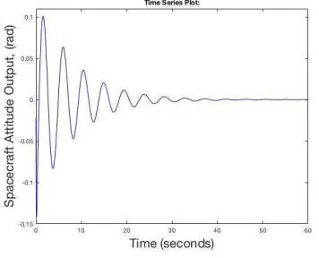
From figure 6 it is seen that the DBL can eliminate the chattering for a while (here upto t = 25s). However, in this technique, the boundary layer width depends on a time determined by ǫ0e−πt and thus, as time approaches infinity,

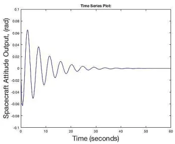
then this term becomes close to zero and the chattering appears again. Nevertheless, the control accuracy (figure 7) is guaranteed.

Figure 6. DBL Technique for Spacecraft’s Attitude Controller Input

Figure 7. DBL Technique for Spacecraft’s Attitude Output

C. SDBL or State-Dependent Boundary Layer Design for SMC

An alternative SDBL design for SMC is proposed in [1]. This will be used as a benchmark for proposed controller design of section V. In SDBL the controller input defined as follows:

u(t) =−σs(t)−c0x1(t)−CAx(t)−ρ(x)f4(s)

+η2

1G

T

P z(t) +η0η1GTP ez(t) (21)

whereP ∈Rn×n

is a positive definite matrix satisfying the Lyapunov inequality (22) withF as in (23),Gas in (24),z(t)

as in (25),η1 as in(26),η0as in (27),ez=z(t)/||z(t)||p and f4(s)as in (28) below.

(−F−σI)T_{P+P(−F−σI)≤0}

(22)

F =



   

0 1 · ·

· 0 1 ·

· · · ·

−c0 · · −cn−1 

   

(23)

G=

0 0 · · · 1T

(24)

z(t) =hRt

0x1dτ x1 · · · xn−1 iT

η1=

ǫ1

ρ0−1

>0 (26)

η0=

ǫ0

ρ0−1

>0 (27)

f4(s) =

s(t)

|s(t)|+ǫ1||z(t)||p+ǫ0

(28)

D. Application of SDBL to a Spacecraft’s Attitude Model

Consider the same parameters value and analysis as in section III-B. Here try ǫ0 = 0.001 and ǫ1 = 0.1 while

||z||p≡

p

z(t)T_{P z(t). Figures 8,9 show that the chattering is}

eliminated and control output accuracy is maintained.

Figure 8. SDBL Technique for Spacecraft’s Attitude Controller Input

Figure 9. SDBL Technique for Spacecraft’s Attitude Output

E. Conclusion

Overall, the DBL design has a simpler controller input compared to the SDBL design which has a more complicated controller input, however the former is not a chattering-free technique. Using SDBL one is able to eliminate the chattering in the controller input but there are many parameters (21) which have to be determined thus increasing the complexity of the controller input algorithm. Hence, an alternative controller input algorithm which has less controller input complexity but is still an improvement of the DBL technique is proposed. Critically, both existing boundary layer methods produce high

control output accuracy for angular velocity in the spacecraft’s attitude.

IV. DECAYINGBOUNDARYLAYERTHOROUGHERROR FEEDBACK(DBLEF)FORSMC

In this section, a minor modification is made to the DBL technique. DBLEF is an initial improvement technique to the DBL. In DBL, the boundary layer width is dependent on time and chattering reappears when time approaches infinity. However, in DBLEF, the boundary layer width is dependent on the error between the actual output and the required output,|d0|. Ideally, in this concept, the boundary layer width

reappears every time |d0| > 0. Hence, the control accuracy

can be guaranteed even when disturbances and uncertainties reappear. Thus, DBLEF is defined below. Controller input and control output accuracy performances are observed by using similar analysis as in Section III.

Algorithm DBLEF: The boundary layer width will be per-manently on and proportional to the error between the desired output and actual output ,|d0|>0. Function f1(s) in (16) is

replaced with f2(s)as in (29).

u(t) =−σs(t)−c0x1(t)−CAx(t)−ρ(x)f2(s) (29)

where the timet in (20) is replaced with 1

|d0| in (30).

f2(s) =

s(t) |s(t)|+ǫ0e

−π |d0|

(30)

Figure 10. DBLEF Technique for Spacecraft’s Attitude Controller Input

Figure 10 shows that the chattering in controller input start around t = 23s when error, |d0 = 0|rad but the chattering

Figure 11. DBLEF Technique for Spacecraft’s Attitude Output

V. DECAYINGBOUNDARYLAYER ANDSWITCHING FUNCTIONTHOROUGHERRORFEEDBACK(DBLSF)FOR

SLIDINGMODECONTROL

In section IV, the DBLEF design shows the chattering pattern is uniformly shaped compare to the DBL but unable to eliminate the chattering in spacecraft’s attitude controller input. Hence, another modification based on DBLEF method is required to achieve the aims of this research. At the end of this section, the controller input and control output accuracy performance are investigated.

A. Proposed SMC algorithm

In figure 6, the DBL for SMC is seen to eliminate the chattering until t = 25s and a new decaying boundary layer thorough error feedback for SMC, the chattering appeared at

t= 23s. Thus, a new decaying boundary layer and switching function thorough error feedback (DBLSF) for sliding mode control is introduced to overcome this problem. This proposed method is less complex compared to the state-dependent boundary layer for SMC technique in Section VI.

Algorithm DBLSF: The boundary layer and switching func-tion in control input (31) will occur when|d0|>0(32). When

|d0|approach to zero, the boundary layer will converge to zero

while switching function will decaying off. Thus the input is given as

u(t) =−σs(t)−c0x1(t)−CAx(t)−ρ(x)f3(s) (31)

where the DBL f1(s)(20) is replaced by the DBLSF

f3(s) =

s(t)e|d−π0|

|s(t)|+ǫ0e

−π |d0|

(32)

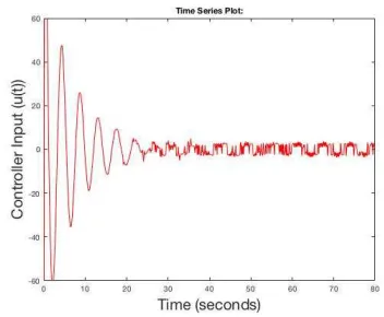
Figure 12 shows that the chattering is totally eliminated in the spacecraft’s attitude controller input while the control accuracy is good, see figure 13. This control method is thus proven able to eliminate the chattering while maintain the control output accuracy.

Figure 12. DBLSF Technique for Spacecraft’s Attitude Controller Input

Figure 13. DBLSF Technique for Spacecraft’s Attitude Output

B. Review of all four SMC algorithms

Overall, four SMC controller input algorithms for space-craft’s attitude control are discussed in this paper. DBL is a simple controller input algorithm (16) but the chattering (figure 6) is reappears when time approaches infinity. SDBL is an improvement to the DBL which produces chattering-free (figure 8) for controller input performance but SDBL requires high complexity (21) controller input algorithm. Hence, the DBLEF and DBLSF are proposed as the alternative methods of SDBL in order to eliminate the chattering for SMC in spacecraft’s attitude system.

The first proposed design, DBLEF is unable to eliminate the chattering (figure 10) since the chattering reappears when

|d0|= 0. Then, DBLSF is proposed to eliminate the chattering

(figure 12). DBLSF performances are comparable to the SDBL design but have a less complex algorithm (31) which thus is suitable to be implemented on small spacecraft operation. On the other hand, all four SMC controller input algorithms produce high control accuracy (figure 7,9,11,13).

VI. CONCLUSIONS ANDFUTURERECOMMENDATIONS

elimi-nate chattering to a level comparable with more complicated methods such as SDBL.

However, in space, there are a few substantive and rigorous scenarios such as fault tolerant cases (actuator degradation scenario where the actuator work efficiency degrades by time (LOE), actuator fault after a certain time scenario (LIUT) and actuator failure for a short time period scenario (FFPT) [13], debris (encompasses by natural (meteoroid) and artificial (man-made) particles) avoidance in space [14] and spacecrafts formation [15]. Future work intends to investigate and justify the capability and robustness of DBLSF design on these scenarios. The spacecraft’s attitude and orientation controller design must be low cost, robust, achieve high precision, high efficiency and low computational in order to be suitable to be implemented on small spacecraft.

VII. ACKNOWLEDGEMENTS

This material is based on work supported by the Malaysia of Higher Education (MOHE) and Universiti Malaysia Perlis (UniMAP). Any opinions, findings, conclusions and recom-mendations expressed in this material are those of the authors and may not reflect those of MOHE and UniMAP.

REFERENCES

[1] M. S. Chen, Y. R. Hwang, and M. Tomizuka, “A state-dependent boundary layer design for sliding mode control,” Automatic Control, IEEE Transactions on, vol. 47, no. 10, pp. 1677–1681, 2002. [2] U. of Concerned Scientists, “Ucs satellite database,”

http://www.ucsusa.org/nuclear-weapons/space-weapons/satllite-database, 2016.

[3] N. S. Hussain, H. H. Basri, and S. Yaacob, “State-dependent boundary layer method for attitude control of satellite,”Jurnal Teknologi, vol. 76, no. 12, 2015.

[4] M. Schmidhuber, S. L¨ow, K. M¨uller, S. Scholz, F. Chatel, R. Faller, and J. Letschnik, “Flight dynamics operations,” inSpacecraft Operations. Springer, 2015, pp. 124–126.

[5] Y. Gao, A. Phipps, M. Taylor, I. A. Crawford, A. J. Ball, L. Wilson, D. Parker, M. Sweeting, A. da Silva Curiel, P. Davies et al., “Lunar science with affordable small spacecraft technologies: Moonlite and moonraker,”Planetary and Space Science, vol. 56, no. 3, pp. 368–377, 2008.

[6] T. Nguyen, J. Leavitt, F. Jabbari, and J. Bobrow, “Accurate sliding-mode control of pneumatic systems using low-cost solenoid valves,”

IEEE/ASME Transactions on mechatronics, vol. 12, no. 2, pp. 216–219, 2007.

[7] A. Sofyalı and E. M. Jafarov, “Integral sliding mode control of small satellite attitude motion by purely magnetic actuation,”IFAC Proceed-ings Volumes, vol. 47, no. 3, pp. 7947–7953, 2014.

[8] X. Liu, P. Guan, and J. Liu, “Fuzzy sliding mode attitude control of satellite,” inDecision and Control, 2005 and 2005 European Control Conference. CDC-ECC’05. 44th IEEE Conference on. IEEE, 2005, pp. 1970–1975.

[9] L. Cao, X. Li, X. Chen, and Y. Zhao, “Minimum sliding mode error feedback control for fault tolerant small satellite attitude control,”

Advances in Space Research, vol. 53, no. 2, pp. 309–324, 2014. [10] S. Staff, “Mars odyssey spacecraft goes into standby after malfunction,”

http://www.space.com/16094-mars-odyssey-orbiter-safe-mode.html, 2012.

[11] P. V. Suryawanshi, P. D. Shendge, and S. B. Phadke, “A boundary layer sliding mode control design for chatter reduction using uncertainty and disturbance estimator,”International Journal of Dynamics and Control, pp. 1–10, 2015.

[12] F. Bacconi, “Spacecraft attitude dynamics and control,”Florence: Flo-rence university, vol. 2006, pp. 1–0, 2005.

[13] L. Cao, X. Chen, and T. Sheng, “Fault tolerant small satellite attitude control using adaptive non-singular terminal sliding mode,”Advances in Space Research, vol. 51, no. 12, pp. 2374–2393, 2013.

[14] D. J. Kessler and B. G. Cour-Palais, “Collision frequency of artificial satellites: the creation of a debris belt,” Journal of Geophysical Re-search: Space Physics, vol. 83, no. A6, pp. 2637–2646, 1978. [15] L. Felicetti and M. R. Emami, “A multi-spacecraft formation approach