Efficient Community Detection

(1)

Efficient Community Detection

Xufei Sun

A subthesis submitted in partial fulfillment of the degree of

Bachelor of Advanced Computing (Honours) at

The Department of Computer Science

Australian National University

(2)

(3)

Except where otherwise indicated, this thesis is my own original work.

(4)

(5)

This work is dedicated to my parents and family, who make the strongest support behind me mentally and economically, during not only the tough individual research

period, but the whole student life. Thank you.

It’s also for my friends, without whom the extreme difficulties, loneliness and my weakness could eat me alive half way, make this dream come true. Yes I finally made

it, and I’m very, very appreciated for everything on this journey. The submission of this thesis eventually ends this fantastic life stage of mine though, the friendship and

memory with you guys, the most precious wealth I gained, accompanies me forever. Special thanks to Xindi Li, Yanning Liu and Renjing Xu.

Finally, I would like to literally kiss and hug myself for one thousand times. This work as well as all the challenges overcome and experience gained along the way, is

dedicated to myself. And this individual research, especially the last few months of it, is the hardest thing I’ve ever attempted or seen. But you make it! You make it! You

(6)

(7)

Acknowledgements

I would like to give my most sincere thank to my supervior, Weifa. It’s his kindness, strictness and experience that makes this work possible.

(8)

(9)

Abstract

Given a large network, local community detection aims at finding the community that contains a set of query nodes and also maximises (minimises) a goodness met-ric. Furthermore, due to the inconvenience or impossibility of obtaining the complete network information in many situations, the detection becomes more challenging.

This problem has recently drawn intense research interest. Various goodness met-rics have been proposed. And most of them base on the statistical features of com-munity structures, such as the internal density or external spareness. However, the metrics often result in unsatisfactory results by either including irrelevant subgraphs of high density, or pulling in outliers which accidentally match the metric for the time being. Further more, when in a highly overlapping environment such as social net-works, the unconventional community structures make these metrics usually end up with a quite trivial detection result.

In our work, we go for a alternative point of view on the formation of the com-munities, namely the assembly of nodes with different roles in the structure. With the new view point, we present two metrics which are proved to perform superiorly in traditional and complex environment respectively. Moreover, on realising a single metric is whatsoever limited in effectiveness as well as scope of application, we raise up a complete framework for the collaboration of metrics in the field, which also lands a base-stone for future innovations.

The experiment results collected from Amazon, DBLP, Youtube and LivingJournal well certifies the effectiveness of the metrics.

(10)

(11)

An Introduction to My Thesis

1.1 Networks, Graphs and Community Structures

[image:15.595.116.331.345.539.2]

1.1.1 Networks in Real Life

Figure 1.1: Protein-Protein Network, reprinted from [Jonsson PF 2006]

When we talk about network, we refer to the concept of a system with a set of com-ponents interacting or interdependent with each other, forming an integrated whole.

A basic knowledge is, where there is any connection or interaction between mul-tiple entities, there is a network. And networks are all around us in life.

For example, the figure 1.1, 1.2, 1.3 respectively notates a network of different kind. Figure 1.1 describes a protein-protein interaction networks. The graph pictures the interactions between proteins in cancerous cells of a rat. Figure 1.2 visualise the data of internet at the AS level. Figure 1.3 depicts the relationship network between two families.

It’s clear that these connections are the bonds that integrate the whole networks. And the study into these connections make great sense if we would like more

(16)

[image:16.595.73.292.108.319.2]

Figure 1.2: Internet Network, reprinted from [Shai Carmi 2007]

Figure 1.3: People Relationship Network

mation about the networks all around us.

1.1.2 Networks and Graphs

Specially, the networks usually can be studied as graphs.

In order to study the networks in depth, an adequate representative form of it is in-dispensable. And this is where the graph theory comes in. The origin of graph theory dates back to 1736. As the amount of understanding and knowledge on graphs ob-tained increases, especially their mathematical properties [Bollob´as 1998], they grad-ually become integral in network researches, as representation of a wide variety of networks in different areas.

[image:16.595.84.282.368.481.2]

(17)

§1.1 Networks, Graphs and Community Structures 3

topics in sociology [Scott 2000]

In recent times, the age of information explosion, the technology dedicated in col-lecting and storing data of unbelievable size evolves at an amazon speed. The human kind is now capable of accessing seas of data which was like a dream. However, this need to deal with such a large number of units, in the order of millions or billions, has produced a deep change in the way graphs are approached [Albert and Barabasi 2002]

Before move on, we are going to formalise definitions for networks and graphs, for the convenience of demonstration in the rest part.

Definition 1. Network, is a system in which the entities connect, interact and influence each other in one way or another. Network would be only referred to as the existed networks in our context.

Definition 2. Graph is a representation of a set of objects where some pairs of objects are connected by links.

1.1.3 Graphs and Basic Concepts

Graphs are essentially data sets stored in the graph database. And now we are going to give a more official definition to them and talk about the details they concerns.

Definition 3. Vertex (also called a ’node’) is a fundamental part of a graph. In many applica-tions the vertex is behind the entity in the real world.

The vertexes can have a name, which we will call the ?key?.

In many applications the vertex is behind the entity in the real world. For exam-ple, in social network like Facebook, one vertex is usually representing a single user in real life; and for amazon commodity network, a node is often associated with a specific good. Besides that, a vertex may also have additional information. We will call this additional information the ?payload.? The quantity of the vertexes belong to a particular graph stands for the amount of concerned objects in it. For example the node number of a regional Facebook graph represents the Facebook user account amount in the area.

Definition 4. Edge (also called an ’arc’) is another fundamental part of a graph. An edge connects two vertices to show that there is a relationship between them in the graph.

(18)

The quantity of edges shows the amount of existing connections between the nodes(objects) of the same graph. For example, the edge number of a company co-operation graph expresses the level of collaborating positiveness between the compa-nies.

Definition 5. The fundamental parts of the graph, namely nodes and edges, may be attached with a certain value demonstrate the difference between two in the graphs, which is called weight.

Particularly, edges can be weighted to demonstrate a key attribute of the connec-tions. For example, the attribute can be the cost to go from one vertex to another; as in a graph of roads that connect one city to another, the weight on the edge might rep-resent the distance between the two cities. Or the length or strength(based on some particular rule) of a friendship on Facebook.

Some of the graphs also contain nodes with different weights. This kind of weight-ing usually showcases the nodes? fit against a given standard. For example, in the PageRank graph, the higher probability(weight) a website(node) with has, the bigger impact it has on the rest of the graph.

Definition 6. The degree of a node is the number of edges connected to the node in the graph.

As far as the graph is concerned, the degree of a node is the number of edges attached to it. And this also mirrors the relational density level of entities in the net-works. Take social networks as examples, the vertex with very high node degree is, without doubt, playing a core role in the group under normal circumstances. At the same time, the node with few connections can be generally viewed as social-inactive.

1.1.4 The Existence of Community Structure

Definition 7. Random graph: The paradigm of disordered graph is the random graph, intro-duced by P. Erdos and A. Renyi in [Erdos and I 1959]. In a random graph, the distribution of edges among the vertices is highly homogeneous. For instance, the distribution of the number of neighbours of a vertex, or degree , is binomial, so most vertices have equal or similar degree. In it, the probability of having an edge between a pair of vertices is equal for all possible pairs

. There are some disciplines in the formation of real life networks, which means that the graphs representing real networks are not usually as regular as frames. Graphs are objects where order coexists with disorder. And they are not random graphs, for they do need to express some level of order and organisation to represent the inho-mogeneities in real-life networks.

(19)

§1.1 Networks, Graphs and Community Structures 5

Definition 8. Community(networks): Communities, also called clusters or modules , are groups of vertices which probably share common properties and/or play similar roles within the graph; usually marked with high concentrations of edges within these groups of vertices, and low concentrations in between

.

If we have a look at the human society, we can find many organisations of clear order, such as military, governments, nations, schools, towns and friend circles. In recent years the online communities have made its appearance in organised groups as well.

Social communities have been studied for a long time [R. Edward Freeman 2004]. And communities also occur in many networked systems from biology, computer sci-ence, engineering, economics, politics, etc. If we have a look back at the network ex-ample given at the first section, we may notice the existence of communities as well, in the form of protein sub-structures, internet communities and families.

1.1.5 Other Special Concepts in Graphs Their Realistic Significance

For the rest of the work, we will give a formal definition and some notations to de-scribe the graph. A graph can be represented by G where G=(V,E). For the graph G, V is a set of vertices and E is a set of edges. Each edge is a tuple (v,w) where w,v?V. We can add a third component to the edge tuple to represent a weight. G=(V,E,W)

Definition 9. Subgraph : A subgraph, H, of a graph, G, is a graph whose vertices are a subset of the vertex set of G, and whose edges are a subset of the edge set of G. In reverse, a super-graph of a super-graph G is a super-graph of which G is a subsuper-graph. A super-graph, G, contains a super-graph, H, if H is a subgraph of, or is isomorphic to G.

Apart from all above, the example graph in the example helps illustrate some other key terms of concern:

Definition 10. Path in a graph is a sequence of vertices that are connected by edges.

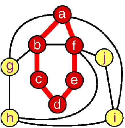
Formally we would define a path as W1,W2,...,Wn such that (Wi,Wi+1)?E for all 1?i?n?1. The unweighted path length is the number of edges in the path, specifically n?1. The weighted path length is the sum of the weights of all the edges in the path. For example in Figure 1.4 the path from node i to node b is the sequence of vertices (i,j,f,b). The edges are (i,j),(j-,f),(f-b).

Definition 11. Cycle in a graph is a path that starts and ends at the same vertex

For example, in Figure 1.4 the path (i,j,f,h) is a cycle. A graph with no cycles is called an acyclic graph.

(20)

[image:20.595.71.290.104.329.2]

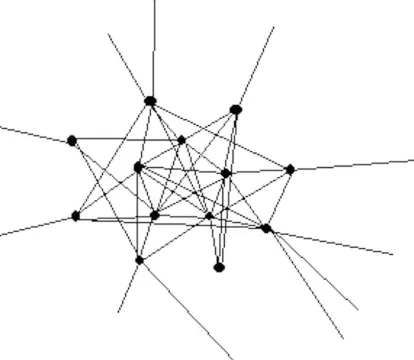
Figure 1.4: node a,b,c,d,e,f and the edges in between make up of a subgraph of the whole graph presented; On the other the entire graph is the super-graph of the graph made up of node a,b,c,d,e,f and the edges in between

Take the graph displayed below an example. We might try to assess which nodes are most similar to which other nodes intuitively by looking at a graph. We would no-tice some important things. It would seem that actors 2,5, and 7 might be structurally similar in that they seem to have reciprocal ties with each other and almost everyone else. Actors 6, 8, and 10 are ”regularly” similar in that they are rather isolated; but they are not structurally similar because they are connected to quite different sets of actors. But, beyond this, it is really rather difficult to assess equivalence rigorously by just looking at a diagram.

Definition 13. Density:the density of a graph(subgraph) is the measurement demonstrating how close the number of edges inside it is to the maximal number of edges for the same set of nodes.

Intuitively, a dense graph is a graph with high density, while on the contrast, a graph with only a few edges, is a sparse graph. The distinction between sparse and dense graphs is rather vague, and depends on the context.

For undirected simple graphs, the graph density is defined as:

D= 2∗|E|

|V|∗(|V|−1)

For directed simple graphs, the graph density is defined as:

D= |E|

(21)

[image:21.595.112.331.109.350.2]

§1.2 Community Structures 7

Figure 1.5: Knoke directed information network [Kno ]

where E is the number of edges and V is the number of vertices in the graph. The maximum number of edges is —V— * (—V— - 1), so the maximal density is 1 (for complete graphs) and the minimal density is 0 [Coleman and Mor´e 1983].

Definition 14. Isolation: Isolation expresses to which extent does a set of nodes(subgraph) in the graph is separated from the rest part, by means of edge amount between nodes within and out

1.2 Community Structures

1.2.1 key features of the community

Community is a widely accepted existence in real-world networks; however in the context of graph, there is still no formal definition of it that is universally accepted; As a matter of fact, the definition often depends on the specific system at hand and/or application one has in mind.

On the other hand, we do have some concrete requirements that any community should satisfy. Firstly, there must be more edges inside the community than edges linking vertices of the community with the rest of the graph. This is the reference guideline at the basis of most community definitions. Besides that, the community has to be connected. It?s obvious that the combination of two disjoint subgraph would hardly make a high-edge-concentration component. And even if they do, the sepa-rated structures would probably make more sense.

(22)

cor-responding nodes to entities belong to the same group in real life, sit in the same communities, share common properties and/or play similar roles in the graphs.

[image:22.595.72.281.188.352.2]

And the picture above showcases some common community structures in net-works.

Figure 1.6: Community structure in social networks [Fortunato 2010]

High (Edge) Density Majority of the statistics definition of the community con-cerns fully or mostly about the edge density. As described in section 1.4, the nodes inside a same community are expected to have more connections between each other. Hence the edge density of the community is one of the most outstanding features of the community. Especially, a subgraph of high edge density is usually found with the existence of considerable cliques(subgraphs in which every node is connected to every other node in the clique). The example is the amazingly huge amount of con-nections between the students from the same college of the same university on social networks.

High Isolation Similar to the high density feature of the communities, according to formation of them in the graphs, the edge amount is expected to be relatively low in between the communities. The idea is intuitive that if a node has a lot of edges associated with the community, the chance is big that it belong to the community as well. Admitted that the node may have even more connections with the outside nodes, the choice of leaving it out of the community still help make a relatively higher isolation(less edges across the boarder). The example is that a collection of Chinese speakers(community) should have much lower connections with the speaker of other languages than with the other native Chinese speaking people.

(23)

community-detection enhancement by proper weighting]. For example, if one needs to contact someone of the same community, he might find multiple ways to get the information about the target from very different people/channels. However, if the target belongs to another community no matter who exactly he is, the chance is that there is a couple of people you have to contact to retrieve the information of the target. Cycle Existence The basic intuition of cycle is similar to that of the shortest path: the nodes in a same community are expected to be connected in multiple ways. And the representation from the graph perspective of the intuition is the existence of the cycle (multiple cycles even) between the nodes in the cluster. The example is, when one needs to contact another belong to the same college, even if he is not able to get in touch with someone who can help him for sure, he will probably succeed in the task through another trail.

Structural Similarity The nodes in a same community should be similar to each other structurally, which means they share a great number of mutual friends. The example is that two students in the same college are expected to have relatively high rate of shared friends(other students in the college). Here the students of the college form the whole community, and the property should be reflected clearly in the graph. Multi-hierarchy Not all communities are equal or of a same hierarchy: a com-munity can contain sub-communities, or be contained by super-communities. The hierarchy is an organisation of actors in some latent space learned from the observed network. And an entity may belong to a series of these communities at the same time. This is a natural phenomenon for clustering and hence, for communities hidden in the graph databases [Qirong Ho 2012]. Many networks in real life exhibits hierar-chy. For example, cold-blooded animals and mammals are large super-communities that can be sub-divided into smaller sub-communities, such as sharks and squid, or toothed whales and pinnipeds. These sub-communities can in turn be divided into even smaller communities (not shown).

Overlapping Since in most networks a single node is allowed (and very usually seen) to be a part of multiple communities at the same time and the communities may not always contain each other, it often appears that very different community pair shared a fraction of the common nodes, also referred to as the overlapping com-munities. Example are everywhere: I am a member of the college computer science association and am a part of the racing club as well. Overlapping is one of the most outstanding disturbing but ubiquitous features of the communities in the graph.

Definition 15. Traditional community structural model, a traditional community is one that obeys the traditional view on the formation of a community, namely a subgraph within the graph with high density and high isolation value.

Definition 16. Traditional graph model: a traditional community is one that obeys the tradi-tional view on the formation of a graph, namely a graph in which high concentration of edge signals the existence of community structures while low in it stands for the part is in between community structures.

(24)

[image:24.595.81.288.213.393.2]

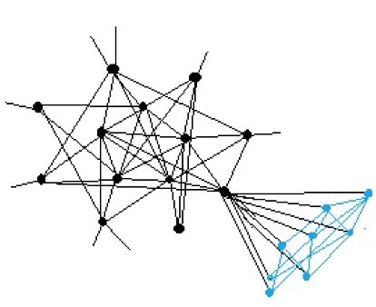
the node is to the outside, the the closer to the edge it would be located in the pic-ture. And we place the node with all adjacencies within the structure in the centre. Further more, the nodes most connected externally (speaking of its edge distribution percentage, same with the following) form the boundary; while the nodes most in-ternally connected make up of the core of the community structure. The definition is qualitative, and for the purpose of demonstration only.

Figure 1.7: traditional community structure model

When a community is barely interacting with and very slightly influenpaced by the outside structures or nodes like this, we say the community is a traditional com-munity structure. And with the features of a comcom-munity, namely the high edge den-sity within and low conductance with the rest graph given above, the nodes on the edges or the furthermost boundaries of the typical communities, is very likely to have a higher internal edge amount than external. Otherwise, due to the internal thin con-nection and unusual high conductance , the node might actually belong to some other communities. For example, under traditional graph model, the node A in figure 1.8 is very likely to be actually a part of the community made up by blue nodes.

Besides the model of subgraph analysed above(conductance of a subgraph can measure how well it is separated from the remaining graph), [Yubao Wu 2015] men-tioned another common-used model, where local community is separated from the remaining graph by a set of low degree nodes. That is to say, the boundary nodes of the communities tend to have low degrees.

The graphs of Amazon and DBLP well represent the model.

1.2.2 why is community important and its application

(25)

[image:25.595.116.323.105.274.2]

Figure 1.8: Outside Node included

always important information whenever we try to manipulate with it. Communities are among the hidden information of the graphs, and contain the potential of help graph express itself better.

Hence communities can have concrete applications. Clustering Web clients who have similar interests and are geographically near to each other may improve the performance of services provided on the World Wide Web, in that each cluster of clients could be served by a dedicated mirror server [Wang 2000].

In the network of purchase relationships between customers and products of on-line retailers (like, e. g., www.amazon.com), getting the idea of the customer groups with similar interests to a large degree help improve the efficient recommendation systems[Agrawal 2011]. And the application is capable of guiding them through the list of items of the retailer and enhancing the business opportunities.

Other than that, the clusters of large graphs can also be used to create data struc-tures in order to generate compact touting tables while the choice of the communi-cation paths is still efficient [clu 2001]. Identifying modules and their boundaries at the same time allows for a classification of vertices, according to their structural po-sition in the modules(this idea is fundamental idea of the node-centric point of view on community structure to be mentioned ). So, vertices with a central position in their clusters, i. e. sharing a large number of edges with the other group partners, may have an important function of control and stability within the group; vertices lying at the boundaries between modules play an important role of mediation and lead the relationships and exchanges between different communities.

(26)

intermediate levels corresponding to work groups, departments and management. Herbert A. Simon has emphasised the crucial role played by hierarchy in the struc-ture and evolution of complex systems [Simon 1991]. The generation and evolution of a system organised in interrelated stable subsystems are much quicker than if the system were unstructured, because it is much easier to assemble the smallest subparts first and use them as building blocks to get larger structures, until the whole system is assembled. In this way it is also far more difficult that errors (mutations) occur along the process.

1.3 what iscommunity detection and its application

As shown in the previous section, the community structure is of great use in many ways however usually implicit. The knowledge about the community structure in a graph requires the process of community detection, which is about exploration, ex-traction and analysis on the graph.

Community detection in graphs is the process of identifying the communities and, possibly, their hierarchical organisation, by only using the information encoded in the graph topology [Fortunato 2010].

When the graph is constrained to be of a small size, containing as many as tens of nodes, the detection process is trivial and fast. Merely with visualised presenta-tion(with software like Graphviz) of the data set and human eyes can one identify the community structures at this scale in no time. However, as the size of data sets in graph database starts to rocket, the detection method evolved accordingly.

At this time and age, the community detection normally indicates the process of inputing the edge information (sometimes with node information) to the computing device, and receiving the formation of community(s) after a series of analysis and computation steps.

Especially, current community detection methods can be roughly classified into two categories, namely global ones and local ones.

Definition 17. global community detection, is a school of community detection methods ded-icated in identifying community structures underlying in the graphs,with always a reference to the whole graph. That means, the global methods needs consideration on the impact on the other parts of graph when determine wether if a subgraph is a community. A representative one belonging to this type is the algorithm of graph partitioning

Definition 18. local community detection is a school of community detection methods aiming at identifying the community structures in the graphs by identifying the formative features of subgraphs(how much this subgraph is like a community). Local methods make the decision with only concern on the properties of current subgraph. The method in this category is nor-mally greedy node addition or greedy node deletion

(27)

§1.4 Motivations 13

1.4 Motivations

1.4.1 Current Challenges

The area of community detection has been studied for several decades, being a par-ticularly intensive interest in recent years. After decades of exhaustive study and experiments, a couple of detection methods with stable and robust performance has already been raised up in the field. However, the new and big challenges keep com-ing, causing problems to existed solutions. The major challenges are as below:

1.4.1.1 Retrieving and storing the information of the entire graph

When the node or edge amount in graph data set are frequently on the order of mil-lions or even bilmil-lions, you will notice the data retrieving and storage becomes a major concern in the process of community detection. In this time of big data the networks are often too large to comprehend and even a simple visualisation of the network is often impossible.[Fast community detection using local neighbourhood search]. This constraint is problematic for networks like the World Wide Web, which for all practi-cal purposes is too large and too dynamic to ever be known fully, or networks which are larger than can be accommodated by the fastest algorithms [Clauset 2005].

Moreover, due to the computational complexity and network bandwidth, this ac-tion of retrievemcent from time to time take much more time than the community de-tection itself, causing an enormous challenge for problems with strict time constraint.

1.4.1.2 The rapid change on the graphs

As described in section 1, the graphs are essentially data sets saved in graph databases. Along with the fast growth in size, the rapid alterations on the existed data sets are causing harsh problems at the same time. It is just too hard to get whole knowledge of the networks evolving quickly or being too big ,such as the Internet [Tiantian Zhang 2012].

1.4.1.3 The problems with seeds

For most of the networks, a large proportion of it is out of our consideration ,we only care about the community structure or other statistical characteristics of some specific nodes. For example, in the book selling network, the purchaser only need the knowledge of books related to some subject, namely the book community which a certain book is in. Hence in the circumstance alike, it would be more appropriate for community detection method to behave as community relegation algorithm of particular nodes of interest [Tiantian Zhang 2012].

1.4.1.4 Dealing with the massive information

(28)

on the massive data. That is also because of most of the detection methods described above (or ever existed) are products from the awareness and manipulations on the complete graph.

For example, finding the optimal partition for a given cost function is in general a difficult problem. Especially, maximising the modularity has been proven to be NP-hard [Brandes 2008]. Hence, different algorithms have been developed to approx-imate the optimal partition of a network. All the existing heuristics designed to extract community structures have to balance the quality of the partition with respect to the time complexity of the algorithm.

When it comes to the community detection tasks with pre-set query node sets, the challenge can get even harder. Due to the attempt to include all the seeds into one community and the intuition of executing the whole algorithm multiple times until the goal is achieved, the detection process would be rather computationally in-tensive for its pre-requirement of detecting all communities, especially for large scale networks [Kwan Hui Lim 2013].

1.4.1.5 The limitation on ability of graphs to demonstrate relationships

Among all the challenges given above, the the limitation of graph database itself is the most serious and almost unsolvable. The act of the graphs to express relationship as edges, while the properties of the relationships as the features given to the edges, is effective to some degree and the only way. However, it can also be quite problematic, so as that under many occasions, the graphdoesn?t represent the relationships(such as friendships /collaboration / chemical reactions) very well.

Furthermore, most current models make the assumption that networks are essen-tially some variation of a random graph, while we know that real networks are far from random on every level, e.g., certain motifs are much more likely than others [Santo Fortunato 2012].

1.4.2 Our Contribution

(29)

§1.5 The formation of the rest parts 15

1.5 The formation of the rest parts

In chapter two, we start with going through some state-of-art algorithms in the com-munity detection field, with the focus on local comcom-munity detection methods. After those, we put the common metrics in local methods under a metric formation frame-work for discussing and comparison; and we talk about the often ignorant way of making better use of the metrics : better designing the stop time for the local algo-rithms. At the end of this chapter, we mentioned a bunch of major problems with he state-of-art metrics.

We then describes our contribution to the field in detail in chapter three. At the beginning of chapter, we raise up a new viewpoint on the community structures, and discusses the cause to current metrics? disability to function in complex environment like social network graphs. Base on this alternative viewpoint, we then raise up two new metrics, with the aims in identifying community structures in traditional graph model and overlapping graph model environment respectively. At the end of this chapter we bring up the SLUD framework, which is able to describe nearly all the current attempts(metric+algorithm) in the field.

(30)

(31)

Chapter 2

Literature Review

2.1 A brief introduction to detection methods

Given the increasing popularity of graph database and the wide-range application, the community detection has been a magnet attracting intensive research interest since its origin as early as 1927, when Stuart Rice looked for clusters of people in small political bodies, based on the similarity of their voting patterns. According to the definition5.2 in introduction part, many of the detection actions are based on the recognisable fea-tures of the community strucfea-tures in the graph, among which the high edge density, high isolation are probably of the most common interest.

And other detection methods are usually associated with a statistical definition of community structure, such as modularity (Q) which was originally introduced by Gir-van and Newman as a stopping criterion for their algorithm. Modularity has rapidly become an essential element of many clustering methods, which is by far the most used and best known quality function. And it represented one of the first attempts to achieve a principle understanding of the clustering problem, and it embeds in its compact form all essential ingredients and questions, from the definition of commu-nity, to the choice of a null model, to the expression of the strength of communities and partitions.

In summary, there have been quite a number of algorithms, based on various the-ories, attempting the task.

Up to today, the initial community detection area has been exhaustively studied and various different but effective-in-some-aspect methods brought about. It?s worth noting that, as the graph size explodes dramatically in the recent decades, nowadays the research focus largely shifts to the time and space consumption of the algorithm.

The focus of our work is on the improvement of seed-centric community detection methods. In the next sections we give out some common methods, of both global and local community detection methods, in the field to begin with.

(32)

2.1.1 global community detection methods

2.1.1.1 graph partitioning

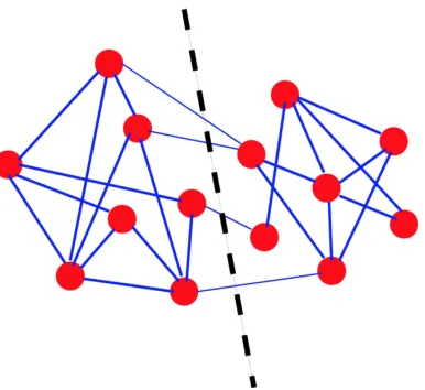
[image:32.595.83.276.265.442.2]

The problem of graph partitioning consists in dividing the vertices in g groups of predefined size, such that the number of edges lying between the groups is minimal. The number of edges running between clusters is called cut size. Graph partitioning is a method mainly dedicated in optimising the isolation property. And the cut size is to be minimised for the target of a high isolation, which is also called the minimum cut problem.

Figure 2.1:Graph partitioning. The dashed line shows the solution of the minimum bisection problem for the graph illustrated, i. e. the partition in two groups of equal size with minimal number of edges running between the groups. Reprinted figure from [Claudio Castellano and Loreto 2009]

One of the best-known solutions in this category is the max-flow min-cut theorem by Ford and Fulkerson [LR Ford 1956] . The theory states that the minimum cut be-tween any two vertices s and t of a graph, i. e. any minimal subset of edges whose deletion would topologically separate s from t , carries the maximum flow that can be transported from s to t across the graph. Hence a equally reasonable partition can be given as the result of a max-flow algorithm on the graph.

2.1.1.2 Hierarchical clustering

(33)

§2.1 A brief introduction to detection methods 19

they are connected or not. At the end of this process, one is left with a new n*n matrix X , the similarity matrix.

Hierarchical clustering techniques aim at identifying groups of vertices with high similarity, and can be classified in two categories: 1. Agglomerative algorithms , in which clusters are iteratively merged if their similarity is sufficiently high; 2. Divi-sive algorithms , in which clusters are iteratively split by removing edges connecting vertices with low similarity. In the context of normal community detection, we often regard the first type as the Hierarchical clustering detection method.

Hierarchical clustering takes advantage of the member similarity feature of the communities, and has very common applications in social network analysis, biology, engineering, marketing, etc.

2.1.1.3 Partitional clustering

Partitional clustering indicates another popular class of methods to find clusters in a set of data points. Here, the number of clusters is preassigned, say k. The points are embedded in a metric space, so that each vertex is a point and a distance mea-sure is defined between pairs of points in the space. The distance is a meamea-sure of dissimilarity between vertices. The goal is to separate the points in k clusters such to maximise/minimise a given cost function based on distances between points and/or from points to centroids , i. e. suitably defined positions in space.

For example, for minimum k-clustering, the cost function here is the diameter of a cluster, which is the largest distance between two points of a cluster. The points are classified such that the largest of the k cluster diameters is the smallest possible. The idea is that the clusters of compact pattern are more likely to form communities.

With different definition of distance, partitional clustering is capable of making use of different features of the communities. For instance, the minimum k-cluster, where the distance stands for essentially the hop number from one node to another, also is based on the existence of massive edges inside the community structures.

2.1.1.4 Divisive Algorithms

The intuition of divisive algorithms is similar to that of graph partitioning, namely to divide the original graph up and get out of it a couple of communities. However, the divisive algorithms selects the edges based on the their chance of being the inter-community edges instead of the effort to minimise cut size. This is the philosophy of divisive algorithms. Hence the crucial point is to find a property of inter-community edges that could allow for their identification.

One of the most famous example of attempts in this field is brought by [Finding and evaluating community structure in networks]. Here edges are selected according to the values of measures of edge centrality , estimating the importance of edges ac-cording to some property or process running on the graph. The steps of the algorithm are:

(34)

centrality: in case of ties with other edges, one of them is picked at random; 3. Re-calculation of centralities on the running graph; 4. Iteration of the cycle from step 2.

One of the metric they use as the standard of inter-community edge identifica-tion is the edge betweenness, by which they are making efforts on the distribuidentifica-tion of shortest path between nodes on the graph(another feature of the communities).

2.1.2 local detection methods

2.1.2.1 Introduction

As defined in introduction part, Local detection methods, don?t require the informa-tion about the whole graph of concern. This school of methods compare a series of subgraphs containing the query nodes, and returns the one that looks most similar to a community structure.

In this time and age of big data, the local community detection method of many variants has become the trend for its superiority in time and space requirements. As described above, a fraction of the detection methods makes use of the accurate statis-tical numbers, such as the subgraph internal edge number, across-subgraph-boarder edge amount and the quantity of shortest path going through a particular edge, in-stead of general but vague features as the guide for community recognition. And the greedy algorithm basically aims at greedily forming a subgraph in order to best suit a given standard ( some selected statistics ) to achieve the community discovery goal.

For example, a greedy approach has been introduced by Blondel et al. [Fast un-folding of communities in large networks], for the general case of weighted graphs. Initially, all vertices of the graph are put in different communities. The first step con-sists of a sequential sweep over all vertices. Given a vertex i , one computes the gain in weighted modularity (Eq. 35 ) coming from putting i in the community of its neigh-bour j and picks the community of the neighneigh-bour that yields the largest increase of Q , as long as it is positive. At the end of the sweep, one obtains the first level partition. In the second step communities are replaced by super-vertices, and two super-vertices are connected if there is at least an edge between vertices of the corresponding com-munities.

2.1.2.2 Starting information of local community detection

(35)

§2.1 A brief introduction to detection methods 21

Up-down local community detection When one has access to the information of the complete graph, one way of detecting the communities containing the seeds is to simply scan all results of a normal community detection method (excluding the local greedy algorithms ) and retrieve the one including the seeds.

However, when it occurs that the seed amount exceeds one and they are organised into different communities by the community detection algorithm(graph partitioning for example), the result can be vague, overly general or inaccurate. Some methods in this type choose to repeat the detection process based on the previous result until the whole seed set being part of a single community, such as [Robust Local Community Detection: On Free Rider Effect and Its Elimination].

Bottom-up local community detection The community detection of this kind, due to the limitation of information, is hardly capable of making use of the features of the community structures. Hence the detection methods falling into this category normally make use of the statistical characteristics of the hidden communities, such as a set of nodes with high internal edge density with relatively low externe density. For the same reason, the greedy algorithm is often associated with the crawler-like seed-centric community detection process.

This is the main research focus in this work.

2.1.2.3 The process of bottom-up local community detection

We begin the description of the process with some basic definitions.

Definition 19. Detected subgraph: detected subgraph is the latest result of the community detection algorithm; especially, in the bottom-up detection methods, it starts as the subgraph made of the query node set; and grows in size every iteration when another node gets pulled in

Definition 20. Ground-truth community: ground-truth communities are the given commu-nity structures in particular graphs. These are often for testing purpose

Definition 21. Candidates: in bottom-up local community detection methods, candidates are the node pool from which the algorithm needs to pick one up and merge it into the detected subgraph every iteration till end

Definition 22. Internal connection amount: internal connection amount is the number of edges between a node of concern and a ground-truth community it belongs to; if the node also belongs to the community, the internal connection amount is usually big in traditional graph models

Definition 23. External connection amount: external connection amount indicates the degree of a node of concern minus its number of connections with current ground-truth community; this is often used in the local detection methods, the internal connection amount is usually small in traditional graph models

(36)

Definition 25. External edge amount: external edge amount indicates the degree of a node of concern minus its number of connections with current detected subgraph; this is often used in the local detection methods as a indicator of external connection amount

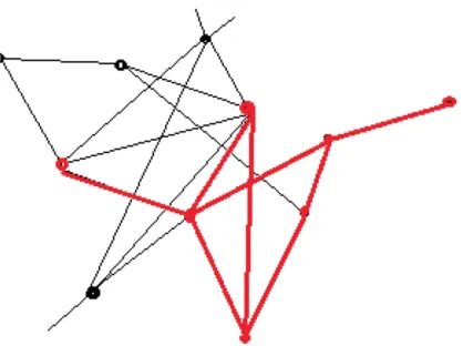
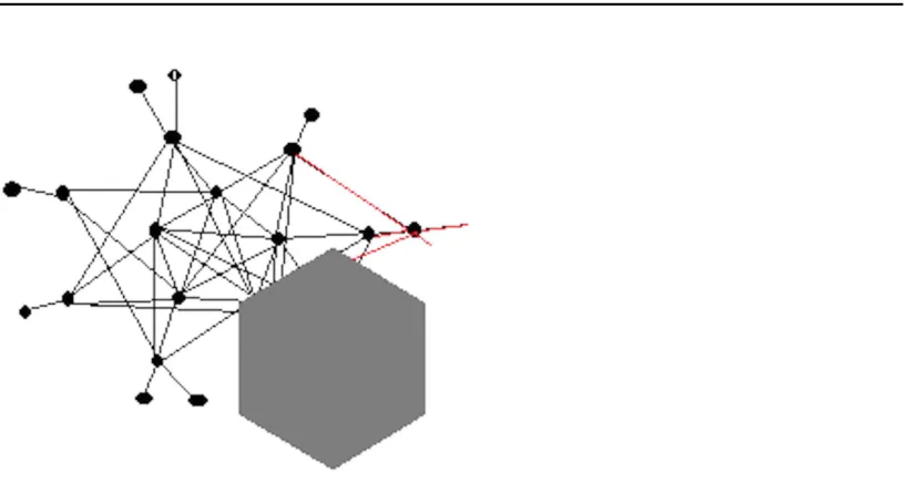
[image:36.595.79.292.300.479.2]

The process of bottom-up local community detection can be described like this: Starting phase: The detection process starts with the query nodes being the detected subgraph. And all the whole neighbour node set makes up the initial candidate node set. Iteration phase: if the inclusion of any node in the current candidate node set wouldn?t make the detected subgraph more similar to a community structure, the detection algorithms stops; otherwise, the algorithm pull in the node making the most benefit for the structure, and update the candidate and detected subgraph information accordingly.

Figure 2.2: Detected subgraph before pulling in in this iteration

[image:36.595.79.288.541.697.2]

(37)

§2.2 The introduction of metric 23

2.2 The introduction of metric

With the knowledge given above, now the main problem is, what defines a subgraph more or less like a community structure? Is there a line of similarity, above which we may say this subgraph makes a community? And this is where metric goes in. Metric is a standard to evaluating the similarity between subgraph structural information and community structure in practical use.

This similarity information may come from the comparison between the detected subgraph and the ground-truth communities. However, this can only be used for testing purpose, because the community information in the graphs is usually un-known(and that is above all why we need to detect the communities!). Especially, for better showing experiment result we give out some indicator stating the effectiveness of a metric(and its associated algorithm).

Suppose that the detected subgraph is notated by S, and the ground-truth commu-nity that contains the query nodes is represented by C.

Definition 26. Precise: the accuracy of the detection result; Precise = |C_|#_S_|S|

Definition 27. Recall : the coverage of the detection result; Recall = |C_|#_C_|S|

Definition 28. Fscore: Fscore = Precise∗Recall Precise+Recall∗2

In the context of local community detection, the criteria of similarity often comes from the outstanding features of community structure, including internal edge den-sity and external isolation and others.

Definition 29. Metric in local community detection process: in our work, we refer to the metric as a full-map function that defines the quantised quality for all subgraphs.

Furthermore, in our context, metric is often the only reference for measuring how good a community the part of the graph is. And if the metric value associated with a particular subgraph meets the definition of community or makes the best-match against the community feature, we say this subgraph is the detected result of our metric on the graph.

2.3 Main Elements Metrics Concern

As described above, the criteria of similarity often comes from the outstanding fea-tures of community structure. In this section we are going to talk about some common elements in concern of metric formulation.

(38)

graphs, as they display big inhomogeneities, revealing the outline of the community structures[community detection in graphs]. A random graph, for instance, is not ex-pected to have community structure, as any two vertices have the same probability to be adjacent, so there should be no preferential linking involving special groups of ver-tices. Therefore, one can dene a null model , i. e. a graph which matches the original in some of its structural features, but which is otherwise a random graph. The null model is used as a term of comparison, to verify whether the graph at study displays community structure or not. The most popular null model is that proposed by New-man and Girvan and consists of a randomised version of the original graph, where edges are rewired at random, under the constraint that the expected degree of each vertex matches the degree of the vertex in the original graph [Newman and Girvan , 2004].

Hence many of the elements in the metric are from statistical difference addressed between the graph formation with clusters and without.

As far as the author is concerned, the common elements metrics contain include but not least:

Internal Edge Quantity The number of edges existed between the node pairs sit-uated inside the subgraph node sets. The internal edge quantity is highly associated with one of the key features of communities: high (edge) density. Hence an recog-nisable relatively high internal edge quantity, normally superior to that of a random graph, is expected with the presence of the community structure.

External Edge Quantity Similar with the internal edge quantity, the number of con-nected node pair with one end inside the subgraph and another outside is expected to differ from the same subgraph belong located in a random graph. The idea is from both another key feature of the community: high isolation, and a comparison to the internal edge quantity. And that is because of the outstanding but homogenised in-ternal and exin-ternal edge quantity hardly make clear of the existence of community structure.

Node Quantity The number of vertexes belonging to the community is another major concern when we design metrics. Though a strict limitation on node number is not common in any networks, but empirically we have the idea that there has to be a range of implicit size setting for any kind of communities, whether it?s social communities or good categories; Other than that, the node quantity makes good sense when it is used in association with internal external edge quantity. The reason is that the internal edge quantity and external edge quantity themselves are tremendously misleading. The collaboration with the edge quantities with the node amount actually produces the edge density, some particular distribution of which is the real indicator of the clustering in the graphs.

There are many other elements can be used to evaluate community structures for sure, for instance the betweenness centrality, the number of cliques included , the structural similarity between nodes inside and the cycle amount between them.

(39)

§2.4 State-of-art Metrics 25

the metrics, the calculation of which needs information about every possible short-est path between every pair of nodes. Another example is the existence of cliques. Although the clique is a relatively good sign of the community structure even in a complex overlapping context, as proved by [Uncovering the overlapping community structure of complex networks in nature and society.] with Clique Percolation Method (CPM), but the slim chance of cliques in considerable sizes containing the seeds makes it not practical at all.

2.4 State-of-art Metrics

And according to [robust Yubao 2015], a goodness metric is usually used to measure whether a subgraph forms a community in local community detection,. The existing goodness metrics for local community detection can be categorised into three classes. The first class optimises the internal denseness of a subgraph, i.e., the set of nodes in a community should be densely connected with each other. Such metrics include the classic density definition [Dense Subgraphs with Restrictions and Applications to Gene Annotation Graphs], edge-surplus [Denser than the densest subgraph: ex-tracting optimal quasi-cliques with quality guarantees], and minimum degree [The community-search problem and how to plan a successful cocktail party]. The sec-ond class optimises both the internal denseness and the external sparseness. That is, the set of nodes in the community are not only densely connected with each other, but also sparsely connected with the nodes that are not in the community. Such metrics include subgraph modularity [Exploring local community structures in large networks], density-isolation [Finding dense and isolated submarkets in a sponsored search spending graph]. The local modularity measures the sharpness of the commu-nity boundary and belongs to the third class [Finding local commucommu-nity structure in networks.]. Using this metric, the set of nodes in the boundary of the community are highly connected to the nodes in the community but sparsely connected to the nodes outside the community.

We now will go through a fraction of the metrics mentioned above.

2.4.1 Internal Denseness

The metrics fall into this category are ones taking merely the edge quantity and node quantity elements into account. The underlying idea is that the set of nodes in a com-munity should be densely connected with each other.

2.4.1.1 Edge Density [MetricS= e_|(_SS_|)]

(40)

can be solved exactly in polynomial time[Dense Subgraphs with Restrictions and Ap-plications to Gene Annotation Graphs].

2.4.1.2 Edge Surplus [

MetricS =e(S)−α∗

!_| S| 2

"

]

However, proved by [C.E. Tsourakakis, F. Bonchi etc] , densest subgraphs(with high-est density) are typically large graphs, with small edge density and large diameter which in many occasion doesn’t make an expected result. So people require another way of making use of the edge density.

A clique is a subset of vertices all connected to each other. And it has been proved that even in a most complex network the emergence of cliques probably lead to the structure of community, since it is very unlikely that inter-community edges form cliques: this idea was already used in the divisive method of [Defining and identifying communities in networks]. However even if in a dense graph, the cliques are not everywhere to be spotted; besides that, the problem of finding whether there exists a clique of a given size in a graph is NP-complete.

Hence [C.E. Tsourakakis, F. Bonchi etc] introduced the concept of quasi-cliques. A

set of vertices S is anαs−quasi−cliquei f e[S](|₂S|),i.e.,i f theedgedensityo f theinducedsubgraphG[S]exceedsathresh

(0, 1).Andtheamounto f internaledgesaseto f nodessharebeyondtheexpectedamounto f thisweakenedcliquede f initioni surplus.Andthesubgraphsthatmaximize fα(S)asarere f erredtoastheoptimalquasi−cliques.

2.4.1.3 Minimum Degree [mindegree]

The internal denseness related metrics discussed above are both upon the average internal degree of the nodes in the extracted community. However, the use of average degree type of metrics in local community detection methods has the drawback of being sensitive to free-riders, namely, irrelevant but dense subgraphs that may be attached to the query nodes and yield unintuitive solutions. For this reason, another a measure, the minimum degree, is attracting a part of research interest.

The density measure fm(H)basedonminimumdegreeisde f inedtobetheminimumdegreeo f anynodeo f VHintheind

(VH,EH).Asanymeasurethatseekstomaximiseaminimum,fmhasthedrawbackthatitissensitivetooutliers.However,it

relatedcommunity,asthemeasure fadoes.

In the seed-centric detection context specially, with the collaboration of excluding nodes that are far from the query nodes, as usually these nodes are less related to the query nodes than those that are nearby, a somewhat satisfactory metric free from the free rider effect can be designed under this scheme[how to organise a cock-tail party].

2.4.2 Internal Denseness and External Sparseness

(41)

§2.4 State-of-art Metrics 27

other, but also sparsely connected with the nodes that are not in the community. And we are going through subgraph modularity and density-isolation here. According to [Finding Dense and Isolated Submarkets in a Sponsored Search Spending Graph], the tasks of identifying dense subgraphs and isolated subgraphs are different; the subgraphs that are most isolated, having the smallest ratio cut score or conductance, tend not to be dense, and the densest subgraphs tend to have large amounts of money crossing their boundaries. More generally, there is some unknown tradeoff between how dense a set can be and how isolated

2.4.2.1 Subgraph Modularity [

MetricS = jnd

(S)

outd(S)

]

[Exploring Local Community Structures in Large Networks ] proposed an interesting metric based on both internal denseness and external sparseness: the subgraph mod-ularity. The modularity M of a sub-graph S in a given graph G is defined as the ratio of its internal degree amount, ind(S), and external degree amount. And obviously the quantity of modularity will increase when sub-graph S has more internal edges and fewer external edges(internal density and external spareness).

On top of this definition,they further give the definition of a proper community

structure: Given a graph G, a sub-graph S⊂Gisamodule/communityi f M >1.Thissimplecommunityde

2.4.2.2 Density Isolation [

MetricS = M(H)−βB(H)−α|H|

]

[Finding Dense and Isolated Submarkets in a Sponsored Search Spending Graph] put forward a metric for subgraphs that are simultaneously dense and isolated. For any subgraph H, M(H) indicated the total edge amount(or weight, as expressed by the original work) within the subgraph; B(H) means the total weight on edges crossing the boundary between the subgraph and the rest of the graph; —H— represents the total number of nodes inside the subgraph. And according to their work, for any fixed value ofα0andβ0,thesubgraphthatoptimisestheob jective f unctioncanbe f ound.

2.4.3 Sharp Boundary

(42)

The emergence of this is also upon one of the main issues with the metrics that takes both internal denseness and external spareness into consideration: at the time communities are big enough, the big portion of total internal edges(neither end locates in the boundary) would make almost all subgraph look good under those metrics.

2.4.3.1 Local Modularity

If we restrict our consideration to those vertices in the subset of C that have at least one neighbour in U, i.e., the vertices which make up the boundary of C, we obtain a direct measure of the sharpness of that boundary. Additionally, this measure is independent of the size of the enclosed community. Intuitively, we expect that a community with a sharp boundary will have few connections from its boundary to the unknown portion of the graph, while having a greater proportion of connections from the boundary back into the local community

2.5 A General Framework of Metric Formation

2.5.1 The Metric Framework, and the relation to the state-of-art metrics

The framework is adapted and improved from the framework raised by [Denser than the Densest Subgraph: Extracting Optimal Quasi-Cliques with Quality Guarantees]. The idea is, the equation containing the very basic elements in metric formation is capable of expressing the constitution of most metrics in local search methods.

Let G = (V,E) be a graph, with —V — = n and —E— = m. For a set of vertices S⊆ V,lete[S]bethenumbero f edgesinthesubgraphinducedbyS.Wede f inethe f ollowing f unction.

2.5.2 A Special Use of the Framework

Our framework is more than capable of describing most of the state-of-metric used in local community detection methods: its essence as a function can be made good use of.

For example, under the framework, to design a algorithm that gets out of a com-munity containing the seeds in a given size from the graph is trivial; furthermore, with proper design such as the application of piecewise function, the metric under the framework can lead to communities of expected size.

MetricS=

$

FunctionA(S) ifx ∈(a,b)

FunctionB(S) otherwise

2.6 The Stopping signal of a local community detection

pro-cess

(43)

[image:43.595.116.526.91.309.2]

§2.6 The Stopping signal of a local community detection process 29

Figure 2.4: When the information about the whole graph topology is incomplete

This signal is particularly essential if we don?t have the detailed information about the whole graph(like figure 2.4), or the time or space constraints doesn’t permit the algorithms running over the whole graph before the result comes out. Given that the seed-centric local bottom-up community detection method without the access to the complete graph information is the main focus of our work, this aspect is therefore of superior significance.

The ability of signalling a proper halt is not well made use of in algorithms, for instance the algorithm described in [local modularity]. The algorithm given in the work would not halt until the detected subgraph has reached a certain size. Figure 2.5 is the example.

[image:43.595.117.326.514.696.2]

(44)

Some of the metrics, such as the first algorithm in 6.1.2, use the possibility of metric value increase as the measure of process: as soon as the metric stops increasing, the detecting process terminates. We will refer to this kind of measure of process as greedy addition in the later part of the work.

Meanwhile, last but not least, a third party of the metric usage exists which utilises some of the elements in its formation instead of the entire equation as the measure of the process. An outstanding example for this is [find local community structure in networks], where the processing terminating signal is a user-setting result node number.

There are often two types of signal indicting the end of the detecting, namely threshold signal and optimum signal.

2.6.1 Threshold Signal

[image:44.595.84.280.399.577.2]

With the threshold signal, a community is ascertained and algorithm stopped as long as the statistical information of the nodes and edges within met a fixed threshold. And the detected subgraph is to be recognised as the community structure. However, it?s evident that in this mode one may get back himself a great number of identified communities unless he stops the detection process manually at some point.

Figure 2.6:In this graph, every K4 subgraph makes a ground-truth community; however, with quasi-clique metric, it?s very likely to include unrelated parts

2.6.2 Optimum Signal

Another commonly accepted mode of signalling community existence is the optimum mode, in which only the optimal result out of all subgraphs encountered is to be re-turned as the community detected.

(45)

ex-§2.7 problems with start-of-art metrics 31

ample. This bottom-up algorithm starts initially with the prescribed seed set and then it keeps adding vertices to the current set S while the objective improves. When no vertices can be added, the algorithm tries to find a vertex in S whose removal may improve the objective. As soon as such a vertex is encountered, it is removed from S and the algorithm re-starts from the adding phase. The process continues until a local optimum is reached.

The work gives additionally another instance in optimum signal mode: The algo-rithm iteratively removes the vertex with the smallest degree from the graph. The out-put is the subgraph produced over all iterations that maximises the metric(measure of goodness).

2.7 problems with start-of-art metrics

2.7.1 Free Rider Effect with Raised Solutions

As defined and systematically proved by [Yubao 2015], most existing metrics tend to include irrelevant subgraphs in the detected local community, also referred to as the free riders. Specifically, if a goodness metric will include the global optimal sub-graph,the subgraph with the largest possible goodness value, in the identified local community, we say this metric causes the global free rider effect; at the same time, if the metric will pull in the local optimal subgraphs, subgraphs whose goodness value is greater than that of their any subgraph, in the identified local community, it is said to be causing the local free rider effect. It?s obvious that the free rider emerges uni-versally with almost every possible local detection metric.

Figure 2.7: universality of free ride effect, table reprinted from [Yubao]

Especially, by definition, the global optimal subgraph also belongs as well to local optimal subgraph.

Definition 30(Global Optimal Subgraph). The global optimal subgraph is the subgraph G[Sm]whosegoodnessvalue f(Sm)f(S),f oranyS ⊂V.

Definition 31(Local Optimal Subgraph). A local optimal subgraph is the subgraph G[Slm]whosegoodnessv

Slm.Thatis,deletinganynode(s)f romalocaloptimalsubgraphwilldecreaseitsgoodnessvalue.Notethatbyde f

(46)

be encountered. Hence, the free rider effect issue in our context equals the local free rider effect as defined in [Yubao]’s work.

[The Architecture of Complexity] points out that hierarchic system structures,

sys-tems composed of interrelated subsyssys-tems, have crucial roles to play in the networks(complex systems). And each of the latter being, in turn, hierarchic in structure until we reach

[image:46.595.75.282.349.484.2]

some lowest level of elementary subsystem. With the self-evident idea in mind that the subsystems presenting in the graphs tend to form internally dense subgraphs, we may further classify the free riders, with the knowledge, into two categories, as the figure 2.8 shows. More specifically, the first type is the dense subgraph that is a part of the ground-truth community at a particular scale; and the second is the dense sub-graph which is not related to the seeds whatsoever. In other word, if the seeds belong to two communities at the same time, one containing another, the free rider of first kind might be included in the community of the larger scale while next to the smaller small one; and the second kind won?t interact, from a ground truth point of view, at any scale.

Figure 2.8:Some of the free riders may be members to community containing query node set but at a larger scale; while some don’t interact with them whatsoever

Intuitively, the actual challenge brought by free riders, to during the detection how do we distinguish between the two kinds of free riders, allow the first kind at a proper time and keep rejecting the member nodes of the second type.