Development and Application of Embedding Methods for the Simulation of Large Chemical Systems

Methods for the Simulation of Large Chemical

Systems

Thesis by

Taylor A. Barnes

In Partial Fulfillment of the Requirements for the Degree of

Doctor of Philosophy

California Institute of Technology Pasadena, California

2015

c

2015

Acknowledgments

I would like to thank my advisor, Prof. Thomas F. Miller III, for his support, advice, and professional example. Throughout my graduate career, his guidance has equipped me to become a more rigorous investigator and a more cogent communicator, and his dedicated mentorship underpins all of the work presented within this dissertation.

I also wish to thank the faculty of the Division of Chemistry and Chemical Engi-neering. In particular, I thank the members of my thesis committee, Prof. William Goddard III, Prof. Mitchio Okumura, and Prof. Brent Fultz, for their supportive advice and insight. I would also like to express my memories of Prof. Aron Kup-permann, who enhanced my development as a scientist and as a person through his thoughtful regard for his students and his willingness to share his unique experiences as a pioneer within the field of quantum mechanics.

I thank all of the members of the Caltech staff, without whom my studies would not have been possible. I especially thank Priscilla Boon and Agnes Tong for their diligent administrative support, and Tom Dunn, Zailo Leite, and Naveed Near-Ansari for providing invaluable technical expertise.

Abstract

The high computational cost of correlated wavefunction theory (WFT) calculations has motivated the development of numerous methods to partition the description of large chemical systems into smaller subsystem calculations. For example, WFT-in-DFT embedding methods facilitate the partitioning of a system into two subsystems: a subsystem A that is treated using an accurate WFT method, and a subsystem B that is treated using a more efficient Kohn-Sham density functional theory (KS-DFT) method.1–3 A primary challenge of WFT-in-DFT embedding is the accurate represen-tation of the embedding potential, which describes the inter-subsystem interactions. In many WFT-in-DFT embedding methods, the embedding potential is treated using the approximations of orbital-free DFT, which can lead to large errors in the result-ing energies. This dissertation describes the development and application of improved embedding methods that enable accurate and efficient calculation of the properties of large chemical systems.

need for a computationally challenging OEP step. The projection-based embedding method has been published in Ref. 11 and in Ref. 12.

Chapter 1 introduces a generalization of the projection-based WFT-in-DFT em-bedding method that is suitable for application to the study of large chemical systems. In the original implementation of the projection-based embedding method, all calcu-lations on subsystem A were performed using the basis set of the full system. When the wavefunction of subsystem A is represented using the basis set of the full system, the computational cost of the WFT calculation on subsystem A increases with re-spect to the size of the full system; this characteristic imposes practical limitations on the applicability of the projection-based embedding method to large chemical sys-tems. In principle, by truncating the basis set representation of the subsystem A wavefunction to include only a subset of the basis functions associated with the full system, it is possible to ensure that the cost of the WFT calculation on subsystem A is independent of the size of the full system. We show that na¨ıve truncation of the basis set associated with subsystem A can lead to large numerical artifacts, and present a method for truncating the basis set associated with subsystem A that en-ables systematic control of these artifacts. The truncation method is applied to both covalently and non-covalently bound test cases, including water clusters and polypep-tide chains, and it is demonstrated that errors associated with basis set truncation are controllable to well within chemical accuracy. This work has been published in Ref. 13.

Bibliography

[1] Cortona, P. Self-Consistently Determined Properties of Solids Without Band-Structure Calculations. Phys. Rev. B 1991, 44, 8454

[2] Wesolowski, T. A.; Warshel, A. Frozen Density-Funtional Approach forAb-Initio Calculations of Solvated Molecules. J. Phys. Chem. 1993, 97, 8050

[3] Govind, N.; Wang, Y. A.; da Silva, A. J. R.; Carter, E. A. Accurate Ab Initio Energetics of Extended Systems Via Explicit Correlation Embedded in a Density Functional Environment. Chem. Phys. Lett. 1998, 295, 129

[4] Goodpaster, J. D.; Ananth, N.; Manby, F. R.; Miller, T. F., III Exact Non-additive Kinetic Potentials for Embedded Density Functional Theory. J. Chem.

Phys. 2010, 133, 084103

[5] Goodpaster, J. D.; Barnes, T. A.; Miller, T. F., III Embedded Density Func-tional Theory for Covalently Bonded and Strongly Interacting Subsystems. J.

Chem. Phys.2011, 134, 164108

[6] Goodpaster, J. D.; Barnes, T. A.; Manby, F. R.; Miller, T. F., III Density Functional Theory Embedding for Correlated Wavefunctions: Improved Methods for Open-Shell Systems and Transition Metal Complexes. J. Chem. Phys.2012, 137, 224113

Pani-agua, M.; Aguado, A. An Inversion Technique for the Calculation of Embedding Potentials. J. Chem. Phys. 2008, 129, 184104

[8] Fux, S.; Jacob, C. R.; Neugebauer; Visscher, L.; Reiher, M. Accurate Frozen-Density Embedding Potentials as a First Step Towards a Subsystem Description of Covalent Bonds. J. Chem. Phys. 2010,132, 164101

[9] Nafziger, J.; Wasserman, A. Density-Based Partitioning Methods for Ground-State Molecular Calculations. J. Phys. Chem. A2014,118, 7623

[10] Libisch, F.; Huang, C.; Carter, E. A. Embedded Correlated Wavefunction Schemes: Theory and Applications. Acc. Chem. Res. 2014, 47, 2768

[11] Manby, F. R.; Stella, M.; Goodpaster, J. D.; Miller, T. F., III A Simple, Ex-act Density-Functional-Theory Embedding Scheme. J. Chem. Theory Comput. 2012, 8, 2564

[12] Goodpaster, J. D.; Barnes, T. A.; Manby, F. R.; Miller, T. F., III Accurate and Systematically Improvable Density Functional Theory Embedding for Correlated Wavefunctions. J. Chem. Phys. 2014,140, 18A507

[13] Barnes, T. A.; Goodpaster, J. D.; Manby, F. R.; Miller, T. F., III Accurate Basis Set Truncation for Wavefunction Embedding. J. Chem. Phys. 2013, 139, 024103

Contents

Acknowledgments iv

Abstract vi

1 Accurate basis set truncation for wavefunction embedding 1

1.1 Introduction . . . 1

1.2 Projection-Based Embedding . . . 2

1.3 AO Basis Set Truncation . . . 6

1.3.1 The Challenges of AO Basis Set Truncation . . . 6

1.3.2 An Improved AO Basis Set Truncation Algorithm . . . 11

1.3.3 Switching Between Orbital Projection and Approximation of the NAKP . . . 15

1.4 Applications . . . 19

1.4.1 WFT-in-HF Truncated Embedding for Polypeptides . . . 19

1.4.2 Embedded MBE . . . 22

1.4.2.1 Water Hexamers . . . 22

1.4.2.2 Polypeptides . . . 26

1.5 Conclusions . . . 30

1.6 Appendix: Water Hexamer Conformations . . . 31

1.7 Appendix: Gly-Gly-Gly Tripeptide Conformations . . . 42

2 Ab initio characterization of the electrochemical stability and solva-tion properties of condensed-phase ethylene carbonate and dimethyl

carbonate mixtures 66

2.1 Introduction . . . 66

2.2 WFT-in-DFT Embedding for Condensed-Phase Systems . . . 68

2.2.1 Overview of Embedding Strategy . . . 68

2.2.2 MD Configurational Sampling . . . 70

2.2.3 Projection-Based Embedding . . . 72

2.2.3.1 Embedding Calculation Details . . . 76

2.2.3.2 Electronic Relaxation of the DFT Region with Re-spect to Oxidation of the Active Region . . . 78

2.2.3.3 Effective Point Charges for the MM Region . . . 80

2.2.3.4 Convergence Tests for the Embedding Cutoffs . . . . 83

2.2.3.5 Convergence Tests for the Basis Set . . . 83

2.3 Results . . . 85

2.3.1 WFT-in-DFT Corrects Over-Delocalization of the Electron Hole 85 2.3.2 Solvation Effects on Different Length Scales . . . 89

2.3.3 Solvent Response to Oxidation . . . 92

2.3.3.1 EC and DMC Solvation Obeys Linear Response . . . 92

2.3.3.2 Failure of Conventional Dielectric Continuum Models for the Treatment of DMC . . . 94

2.3.3.3 Importance of Quadrupolar Interactions in DMC Sol-vation . . . 98

2.4 Conclusions . . . 103

2.5 Appendix: Benchmarking the Electronic Relaxation Calculations . . . 104

List of Figures

1.1 Schematic of the BK-1 water hexamer . . . 7 1.2 µ-dependence of the embedding errors for the BK-1 water hexamer . . 8 1.3 Demonstration of the effects of the parameter τ for the BK-1 water

hexamer . . . 14 1.4 Convergence of the errors for the BK-1 water hexamer with respect to

size of the truncated basis set . . . 17 1.5 Diagram of the GGGG tetrapeptide . . . 19 1.6 Demonstration of the effects of the parameterτfor the GGGG tetrapeptide 20 1.7 Convergence of the errors for the GGGG tetrapeptide with respect to

size of the truncated basis set . . . 21 1.8 Accuracy of supermolecular EMBE2 calculations for determining the

relative conformational energies of water hexamers . . . 24 1.9 Accuracy of truncated EMBE2 calculations for determining the relative

conformational energies of water hexamers . . . 25 1.10 Schematic of the GGG, VPL, and YPY tripeptides . . . 27 1.11 Accuracy of supermolecular and truncated EMBE2 calculations for

var-ious conformations of the GGG tripeptide . . . 28

2.1 Summary of the embedding protocol . . . 68 2.2 Contribution of the electronic relaxation energy of subsystem B to the

2.4 Distribution of vertical IEs of isolated EC and DMC molecules . . . 85 2.5 Analysis of the extent of electron hole delocalization in EC dimers . . . 87 2.6 Contribution of the solvent to the vertical IE of liquid-phase EC . . . . 90 2.7 Importance of the WFT-level treatment of subsystem A for liquid-phase

EC and DMC . . . 91 2.8 Equilibrium probability distributions of the vertical IE of EC in both

the reduced EC system and oxidized EC+ _{system . . . . 93} 2.9 Equilibrium probability distributions of the vertical IE of several systems

of EC and DMC . . . 95 2.10 Examination of the accuracy of the electrostatic model for estimation of

the vertical IE energy of EC and DMC molecules. . . 99 2.11 Analysis of the contribution of intermolecular dipolar and quadrupolar

electrostatic interactions to the vertical IE of liquid-phase EC and DMC 101 2.12 Demonstration of the accuracy of the electronic relaxation protocol . . 105 2.13 Demonstration that the conclusion that DMC quadrupolar interactions

List of Tables

1.1 List of water molecules comprising the set of border atoms for each value of RO-O in Fig. 1.3(c) . . . 13 1.2 Summary of the EMBE2 results on the water hexamer test set . . . 26 1.3 Summary of the EMBE2 results for the Gly-Gly-Gly tripeptide . . . . 29 1.4 Summary of the EMBE2 results for the VPL tripeptide, the YPY

tripep-tide, and the GGGG tetrapeptide . . . 29

Chapter 1

Accurate basis set truncation for

wavefunction embedding

1.1

Introduction

The computational cost of electronic structure calculations has motivated the devel-opment of methods to partition the description of large systems into smaller subsys-tem calculations. Among these are the QM/MM,1–6 ONIOM,7,8 fragment molecular orbital (FMO),9–15 and WFT-in-DFT embedding16–30 approaches, which allow for the treatment of systems that would not be practical using conventional wavefunc-tion theory (WFT) approaches. In particular, WFT-in-DFT embedding utilizes the theoretical framework of density functional theory (DFT) embedding to enable the WFT description of a given subsystem in the effective potential that is created by the remaining electronic density of the system.16–30 _{We recently introduced a simple,} projection-based method for performing accurate WFT-in-DFT embedding calcula-tions30that avoids the need for a numerically challenging optimized effective potential (OEP) calculation24,25,31–34via the introduction of a level-shift operator. It was shown that this method enables the accurate calculation of WFT-in-DFT subsystem correla-tion energies, as well as many-body expansions (MBEs) of the total WFT correlacorrela-tion energy.30

the supermolecular basis, such that the embedded subsystem electronic structure calculation is performed in the atomic orbital (AO) basis set of the full system.30 From a computational efficiency standpoint, this is not ideal. Although the embedded subsystem calculation has fewer occupied MOs than that performed over the full system, the number of virtual MOs is not reduced. The cost of traditional WFT methods typically depends more strongly on the number of virtual MOs than on the number of occupied MOs; for example, the CCSD(T) method scales as o3_v4_{, where o} and v indicate the number of occupied and virtual MOs, respectively.35 _Truncation of the AO basis set in which the embedded subsystem is represented would lead to a reduction in the number of virtual MOs, thus significantly reducing the computational cost of the embedded subsystem calculation.

In the current work, we present a method for accurately truncating the AO basis set for embedded subsystem calculations, and we demonstrate its accuracy for both covalently and non-covalently bound systems. It is shown that this approach provides a means of controlling truncation errors and of systematically switching between ex-isting approximate embedding methods and rigorous projection-based embedding. Furthermore, we present both embedded WFT calculations and embedded MBE cal-culations for molecular clusters and polypeptides.

1.2

Projection-Based Embedding

incre-mental scheme of Stoll et al.,38 _{the region method of Mata et al.,}39 _{and Henderson’s} embedding scheme.40

In projection-based embedding, an SCF calculation (either HF or Kohn-Sham (KS)-DFT) is first performed over the full system. The resulting set of occupied MOs, {φi}, is then optionally rotated before it is partitioned into sets {φi}A and

{φi}B, which correspond to subsystems A and B, respectively. These two sets of

orbitals are used to construct the respective subsystem density matrices in the AO basis set,γA _{and γ}B_.

In the embedded subsystem calculation, orthogonality between the subsystem MOs is enforced via the addition of a projection operator, PB, to the subsystem A embedded Fock matrix, such that

fA=hA in B[γA, γB] +g[γ_embA ], (1.1)

where the embedded core Hamiltonian is

hA in B[γA, γB] =h+g[γA+γB]−g[γA] +µPB, (1.2)

h is the standard one-electron core Hamiltonian, g includes all two-electron terms, and µ is a level-shift parameter; γA

emb is the density matrix associated with the MO eigenfunctions of fA. The projection operator is given by

P_αβB ≡ hbα|

( X

i∈B

|φiihφi|

)

|bβi, (1.3)

kinetic energy vanish in this limit. The embedded SCF calculation using the Fock matrix in Eq. 2.4 is iterated to self-consistency with respect to γA

emb. The energy of the resulting SCF-in-SCF embedding calculation is then

ESCF[γembA ;γ A

, γB] =ESCF[γembA ] +ESCF[γB] +ESCFnad[γ A

, γB]

+ tr(γ_embA −γA)(hA in B[γA, γB]−h),

(1.4)

whereESCFis the SCF energy andESCFnad[γA, γB] is the non-additive interaction energy between the densities γA and γB. The last term in Eq. 1.4 is a first-order correc-tion to the difference between E_SCFnad[γA, γB] and E_SCFnad[γ_embA , γB].25 For µ → ∞, the SCF-in-SCF embedding energy is identical to the energy of the corresponding SCF calculation performed over the full system; as a result, the projection-based approach is numerically exact for SCF-in-SCF embedding calculations. In our previous work,30 we introduced an additional perturbative correction to the SCF-in-SCF energy to account for the finite value of µ in a given computation; this correction is typically far smaller than the energy differences discussed in the current paper and is thus neglected throughout.

For the special case of DFT-in-DFT embedding, the two-electron potential terms include contributions from the electron-electron electrostatic repulsion and exchange-correlation, such that

g[γA+γB] =J[γA+γB] +vxc[γA+γB]. (1.5)

The associated non-additive interaction energy is

where

Jnad[γA, γB] = Z

dr1 Z

dr2

γA_(1)γB₍₂₎

r12

(1.7)

and

E_xcnad[γA, γB] =Exc[γA+γB]−Exc[γA]−Exc[γB]. (1.8)

Evaluation ofJnad[γA, γB] is straightforward, and although the exact form ofE_xcnad[γA, γB] is not known, approximate exchange-correlation (XC) functionals are well-established. Eq. 1.6 does not include any contributions from the non-additive kinetic energy (NAKE), Tnad

s [γA, γB], as this term vanishes due to the explicit mutual orthogonal-ization of the subsystem MOs. Similarly, the special case of HF-in-HF embedding is obtained by replacing the exchange-correlation potential and energy functionals,

vxc[γA+γB] in Eq. 1.5 and Excnad[γA, γB] in Eq. 1.6, with the corresponding HF exchange terms.30

Projection-based embedding also allows for WFT-in-SCF embedding, in which subsystem A is treated at the WFT level and subsystem B is described at the SCF level.30_{This simply involves replacing the standard one-electron core Hamiltonian in} a WFT calculation with the embedded core Hamiltonian of Eq. 2.5. The electronic energy from the WFT-in-SCF approach is

EWFT[ΨA;γA, γB] =hΨA|HˆA in B[γA, γB]|ΨAi

+ESCF[γB] +ESCFnad[γ A_{, γ}B_]

−tr

γA(hA in B[γA, γB]−h)

,

(1.9)

trγA emb(h

A in B_[γA_{, γ}B_]−h)

is included in the first term of Eq. 2.7, it does not appear in the last term, unlike Eq. 1.4.

1.3

AO Basis Set Truncation

1.3.1

The Challenges of AO Basis Set Truncation

Practical implementation of WFT-in-DFT embedding for large systems requires trun-cation of the AO basis set for the subsystem that is described at the WFT level of theory. We now illustrate the challenges of this task by analyzing the errors that arise from truncation of the AO basis set; in particular, we show that significant numerical errors can arise due to the difficulty of constructing MOs in the truncated AO basis set that are sufficiently orthogonal to the projected MOs in subsystem B.

Calculations utilizing the truncated AO basis set are referred to as truncated em-bedding calculations, as opposed to supermolecular emem-bedding calculations for which the AO basis set is not truncated. Specifically, the truncated embedding calculation for subsystem A is performed within an AO basis set, {bα}A, that is a subset of the AO basis set for the full system, {bα}. All calculations are performed using the

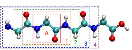
implementation of projection-based embedding in the Molpro software package.44 As a starting point, we present a set of HF-in-HF supermolecular embedding calculations against which truncated embedding calculations can be compared. A closed-shell HF calculation is performed on a water hexamer in the BK-1 geometry45 using the cc-pVDZ basis set;46,47 _{all geometries employed in this study are provided} in the appendices (Section 1.6-1.8). We number the molecules of the water hexamer as shown in Fig. 2.1(a). Following Pipek-Mezey localization of the canonical HF MOs,48subsystem partitioning is performed by assigning the five MOs with the largest Mulliken population on water molecule 1 to {φi}A; the remaining MOs are assigned

1


2
 4
 6


5
 3


Border


Ac/ve


Distant


(a)
 (b)


Figure 1.1: (a) The BK-1 water hexamer, with molecule numbering indicated. (b) Illustration of the atom sets defined in Section 1.3.2, with one possible choice of the active, border, and distant atoms indicated.

for the level-shift parameter µ.

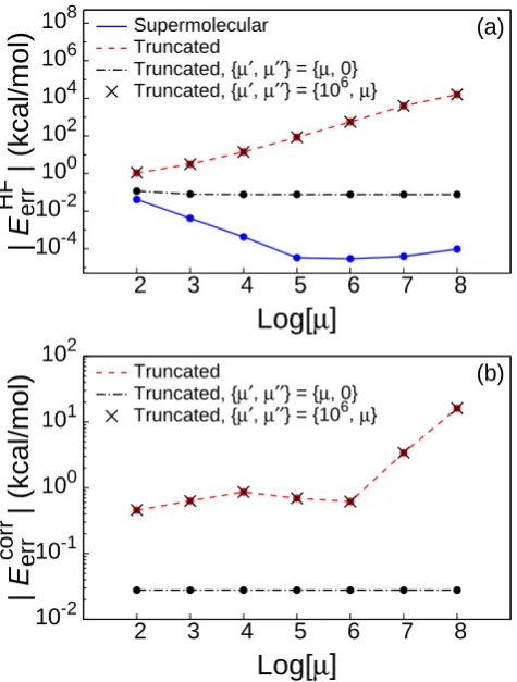
The solid line in Fig. 1.2(a) presents theµ-dependence of the HF-in-HF embedding error,

E_errHF≡E_embHF −E_fullHF, (1.10)

where E_embHF is the energy of the HF-in-HF embedding calculation, and E_fullHF is the energy of the HF calculation performed over the full system. As previously ob-served,30 _{the error in the SCF-in-SCF supermolecular embedding calculations is} sub-microhartree and varies little with respect toµ over several orders of magnitude.

The dashed line in Fig. 1.2(a) shows the results of a naive HF-in-HF truncated embedding calculation, in which {bα}A is defined to include only the AO basis func-tions centered on the atoms in water molecules 1, 2, and 3. Calculation of the HF MOs, {φi}, and the subsystem density matrices, γA and γB, is performed in the

su-permolecular basis, {bα}. The embedded core Hamiltonian in Eq. 2.5 is initially

constructed in the supermolecular basis, after which all matrix elements in hA in B

that do not correspond to the truncated AO basis are discarded. The embedded calculation for subsystem A is then performed in the truncated AO basis. Unlike the supermolecular case, Fig. 1.2(a) illustrates that these naive truncated embedding calculations (solid) produce energies which strongly vary with respect toµ.

10-4 10-2 100 102 104 106 108

2 3 4 5 6 7 8

|

E

HF err

| (kcal/mol)

Log[

µ

]

(a)

Supermolecular Truncated

Truncated, {µ′, µ′′} = {µ, 0} Truncated, {µ′, µ′′} = {106, µ}

10-2 10-1 100 101 102

2 3 4 5 6 7 8

|

E

corr err

| (kcal/mol)

Log[

µ

]

(b)

Truncated

Truncated, {µ′, µ′′} = {µ, 0} Truncated, {µ′, µ′′} = {106, µ}

MOs in subsystem B are projected. In these results, the projection operator is parti-tioned into two parts, PB0

αβ and PB

00

αβ, each with a different level-shift parameter. The

partitioned projection operators are defined as

P_αβB0 ≡ hbα|

( X

i∈B0

|φiihφi|

)

|bβi (1.11)

and

P_αβB00 ≡P_αβB −P_αβB0. (1.12)

The summation in Eq. 1.11 is over the set of MOs {φi}B0, which is a subset of{φi}B. Eq. 1.12 corresponds to the projection of the set of MOs, {φi}B00, that consists of all subsystem B MOs that are not included in {φi}B0. The resulting embedded core Hamiltonian (from Eq. 2.5) is

hA in B =h+g[γA+γB]−g[γA] +µ0PB0

+µ00PB00.

(1.13)

In these calculations, a particular MO in {φi}B is assigned to {φi}B0 only if its com-bined Mulliken population on the basis functions centered on water molecules 2 and 3 is greater than 0.5, such that only the 10 (doubly-occupied) MOs in subsystem B that are localized on water molecules 2 and 3 are included. Setting µ0 to a positive value while µ00= 0 corresponds to projecting only the MOs that are localized within the truncated AO basis set, {bα}A.

effect of changing µ00 while leavingµ0 fixed at 106_.

The results from Fig. 1.2(a) may seem counterintuitive, since the overlap between

{φi}B00 and the truncated AO basis set is much smaller than the overlap between

{φi}B0 and the truncated AO basis set; it might be expected that projection of the

MOs in {φi}B00 would have little impact on the truncated embedding calculation. However, the observed behavior can be understood in terms of the difficulty of con-structing MOs that are orthogonal to {φi}B00 within the truncated Hilbert space of subsystem A. Because the orbitals that are projected by µ00 do not strongly overlap with the basis functions accessible to subsystem A, achieving orthogonality between the subsystem A MOs and {φi}B00 places severe demands on the diffuse functions of the truncated AO basis set; in the supermolecular basis set, this difficulty is elimi-nated. For cases in which the truncated basis set is insufficiently flexible to construct MOs that are effectively orthogonal to {φi}B00, the error in the truncated embedding calculation increases linearly with the level-shift parameter µ00.

Fig. 1.2(b) shows that the same trends hold for WFT-in-HF embedding. The fig-ure plots the truncation error in the correlation energy of the WFT-in-HF embedding calculations,

E_errcorr≡E_trunccorr −E_supercorr , (1.14)

whereE_trunccorr is the correlation energy of a WFT-in-HF truncated embedding calcula-tion (i.e., the difference between the WFT-in-HF and HF-in-HF embedding energies) and E_supercorr is the correlation energy of a WFT-in-HF supermolecular embedding cal-culation obtained with the same choices of {φi}B and µ0. In the supermolecular embedding calculation, all members of {φi}B are assigned to {φi}B0. The correlation energy is defined in the standard way:

The WFT calculations in Fig. 1.2(b) are performed at the CCSD(T) level of theory,49 and the subsystems are partitioned as in the corresponding HF-in-HF embedding calculations. As observed for the HF-in-HF truncated embedding calculations, the errors of the CCSD(T)-in-HF truncated embedding calculations exhibit very little dependence on µ0 and strong dependence on µ00.

Taken together, the results in Fig. 1.2 illustrate that significant numerical arti-facts arise from the enforcement of orthogonality between the MOs of subsystem A in the truncated basis set and the MOs of subsystem B that are localized outside of the truncated AO basis set. Projection of {φi}B00 leads to significant errors, as well as dependence upon the level-shift parameter (Figs. 1.2(a) and 1.2(b), crosses). This problem is avoided by settingµ00 = 0 in Eq. 1.13, resulting in truncated embed-ding calculations that exhibit both good accuracy and very little dependence on the remaining level-shift parameter, µ0 (Figs. 1.2(a) and 1.2(b), dashed-dotted curve).

1.3.2

An Improved AO Basis Set Truncation Algorithm

Incorporating the observations from Section 1.3.1, we now present an algorithm for AO basis set truncation in projection-based embedding that avoids dependence on the level-shift parameters and that yields controllable error with respect to the size of the truncated basis set. Truncated embedding calculations require specification of (i) the subsystem B MOs, {φi}B, (ii) the set of AO basis functions in which subsystem A is solved,{bα}A, and (iii) the set of subsystem B MOs that are to be projected,{φi}B0. In the new algorithm, these specifications are made via the respective selection of (i) a set of “active atoms” that are associated with subsystem A, (ii) a set of “border atoms” that lie at the interface of subsystems A and B, and (iii) an MO overlap threshold parameter, τ.

localiza-tion of the MOs; we employ the Pipek-Mezey localizalocaliza-tion method throughout this paper. An MO is assigned to{φi}B if and only if the atom on which the MO has the largest Mulliken population is not an active atom. For the BK-1 water hexamer, one example of a choice of active atoms is provided in Fig. 2.1(b).

The set of border atoms is used to determine {bα}A. Only AO basis functions centered on either an active atom or a border atom are included in {bα}A. Any

atom that is not assigned to either the set of active atoms or the set of border atoms is assigned to the set of “distant atoms.” The special case in which no atoms are included in the set of border atoms is equivalent to using the monomolecular basis, while the special case in which no atoms are included in the set of distant atoms corresponds to using the supermolecular basis. An example of one possible choice of border atoms is given in Fig. 2.1(b).

The overlap threshold parameter τ is used to determine {φi}B0. A given MO in

{φi}B is assigned to {φi}B0 if it exhibits a combined electronic population on the

border atoms, Ni, such that |Ni| > τ; for the purpose of determining the electronic

population on individual atoms, we employ Mulliken population analysis throughout this paper. For the special case of τ = 0, all MOs in {φi}B are assigned to {φi}B0, whereas sufficiently large values of τ correspond to assigning no MOs to {φi}B0.

number of MOs in {φi}B (Fig. 1.3(a)). As more MOs are added to{φi}B0, the error increases substantially (Fig. 1.3(b)); this is consistent with the previous observation that projection of the subsystem B MOs not localized within {bα}A results in large errors (Fig. 1.2, crosses). For very large values ofτ, the error in Fig. 1.3(b) increases substantially due to “charge leakage,” which is discussed later in this section and in Section 1.3.3.

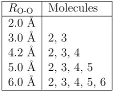
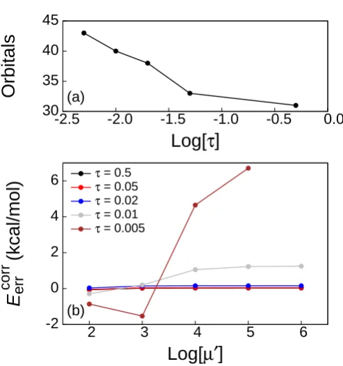
Fig. 1.3(c) illustrates the sensitivity of HF-in-HF truncated embedding calcula-tions to the size of the truncated AO basis set. The calculacalcula-tions use the set of active atoms indicated in Fig. 2.1(b) and{µ0, µ00, τ}={106_{,0,0.5}. The set of border atoms} for each calculation is determined through the use of a cutoff parameter, RO-O. If the oxygen atom of a particular water molecule is within a distance RO-O of an ac-tive oxygen atom, all atoms in that water molecule are included in the set of border atoms; the set of border atoms for each value of RO-O in Fig. 1.3(c) is indicated in Table 1.1. Fig. 1.3(c) illustrates that the truncated embedding calculation converges rapidly with respect to the number of border atoms.

RO-O Molecules 2.0 ˚A

3.0 ˚A 2, 3 4.2 ˚A 2, 3, 4 5.0 ˚A 2, 3, 4, 5 6.0 ˚A 2, 3, 4, 5, 6

Table 1.1: List of water molecules, the atoms of which comprise the set of border atoms for each value ofRO-O in Fig. 1.3(c). AtRO-O = 3.0 ˚A, the set of border atoms is the same as that shown in Fig. 2.1(b).

5 10 15 20 25 30

-8 -7 -6 -5 -4 -3 -2 -1

Orbitals

Log[

τ

]

-8 -7 -6 -5 -4 -3 -2 -1

|

E

HF err

| (kcal/mol)

Log[

τ

]

2 3 4 5 6

|

E

HF err

| (kcal/mol)

R

(Å)

allows for the improper transfer of electron density from the embedded subsystem to the surrounding environment.50–52 _{As we show in the Section 1.3.3, this problem can} be remedied in the context of truncated projection-based embedding.

1.3.3

Switching Between Orbital Projection and

Approxima-tion of the NAKP

To address the problem of charge leakage in truncated embedding calculations employ-ing diffuse basis sets, we include a simple modification to the truncated embeddemploy-ing algorithm from Section 1.3.2. Because that algorithm does not fully enforce mutual orthogonality between the subsystem A MOs and the MOs in{φi}B00, the NAKE be-tween the corresponding electronic densities is non-zero. Accounting for this NAKE contribution requires modification of the embedded core Hamiltonian in Eq. 1.13, such that

hA in B ≈h+g[γA+γB]−g[γA] +µ0PB0

+vA_NAKP[γA, γB00],

(1.16)

where γB00 _{is the density matrix corresponding to the subsystem B MOs in {φ}

i}B00, and the non-additive kinetic potential (NAKP) is

vA_NAKP[γA, γB00] =vTs[γ A

+γB00]−vTs[γ A

]. (1.17)

The corresponding SCF-in-SCF energy from Eq. 1.4 is then

ESCF[γembA ;γA, γB]≈ESCF[γembA ] +ESCF[γB]

+E_SCFnad[γA, γB] +T_snad[γA, γB00]

+ tr(γ_embA −γA)(hA in B−h),

where

T_snad[γA, γB00] =Ts[γA+γB 00

]−Ts[γA]−Ts[γB 00

], (1.19)

and the corresponding WFT-in-SCF energy from Eq. 2.7 is

EWFT[ΨA;γA, γB]≈ hΨA|HˆA in B|ΨAi

+ESCF[γB] +ESCFnad[γ

A_{, γ}B_{] +T}nad s [γ

A_{, γ}B00_]

−tr

γA(hA in B−h)

.

(1.20)

By construction, the overlap between the MOs in subsystem A and {φi}B00 is small; it can thus be expected that currently available approximations to the kinetic energy functional will provide an adequate description of the NAKE.

If all atoms are included in either the set of active or border atoms and if τ

is sufficiently small, this approach corresponds to supermolecular projection-based embedding and involves no approximate KE functionals. In the other extreme, if no atoms are included in the set of border atoms, then no MOs are projected and the approach corresponds to the familiar case of monomolecular DFT embedding with the use of an approximate KE functional. The protocol in Eqs. 1.16-1.19 thus allows for the systematic switching between monomolecular DFT embedding and projection-based supermolecular embedding via modulation of τ and the set of border atoms.

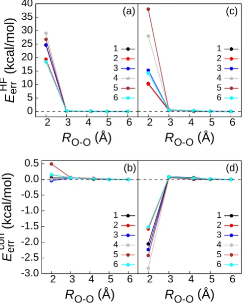
To demonstrate this switching, Fig. 1.4 presents a series of truncated embedding calculations on the BK-1 water hexamer using the cc-pVDZ basis set. In each calcula-tion, the active atoms correspond to one of the water molecules,{µ0, τ}={106_,0.5}, andvA

NAKP[γA, γB 00

0 5 10 15 20 25 30 35 40

2 3 4 5 6

E

HF err

(kcal/mol)

R

(Å)

2 3 4 5 6

E

corr err

(kcal/mol)

R

(Å)

2 3 4 5 6

R

(Å)

2 3 4 5 6

R

(Å)

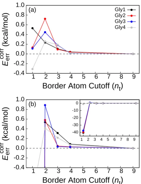
In Figs. 1.4(c) and 1.4(d), these calculations are repeated using the larger aug-cc-pVDZ basis set. Again, the results converge rapidly with respect to the number of border atoms. However, the results in Figs. 1.4(c) and 1.4(d) contrast with those discussed in Section 1.3.2, for which truncated embedding with the larger basis set failed due to charge leakage. We thus find that inclusion of the NAKP between the subsystem A MOs and the MOs in {φi}B00 helps to mitigate the issue of charge leakage when basis set truncation is employed. This finding is consistent with earlier observations that monomolecular DFT embedding is a useful strategy for mitigating charge leakage.55–57

Finally, we note that Eqs. 1.16 and 1.18 can be regarded as a pairwise approxi-mation,31,32 such that

T_snad[γA, γB0 +γB00]≈T_snad[γA, γB0]

+T_snad[γA, γB00].

(1.21)

In the limit of µ0 → ∞, the embedded subsystem MOs and the MOs in {φi}B0 are constrained to be mutually orthogonal for all γA_{; subject to this constraint,}

Tnad

s [γA, γB 0

] = 0 for all γA_{, and}

vA_NAKP[γA, γB0] = δT nad

s [γA, γB 0

]

δγA = 0. (1.22)

Therefore, the only nonzero contribution to the NAKP is vA_NAKP[γA, γB00] (Eq. 1.16), and the only contribution to the NAKE is Tnad

s [γA, γB 00

1


A


2
 3 4

Figure 1.5: The Gly-Gly-Gly-Gly tetrapeptide, with the set of active atoms composing the Gly2 residue (solid red box). Each of the dashed boxes indicates the union of the sets of active and border atoms for the corresponding value of nt; any atoms outside of the boxes are included in the set of distant atoms.

1.4

Applications

1.4.1

WFT-in-HF Truncated Embedding for Polypeptides

For a more demanding illustration of the truncated embedding approach presented in Section 1.3.3, we consider the Gly-Gly-Gly-Gly tetrapeptide. The optimized geometry of the tetrapeptide is determined at the HF/cc-pVDZ level, with all backbone dihedral angles constrained to 180◦. For each of the truncated embedding calculations in this section, the set of active atoms consists of the atoms of one of the four glycine residues. The set of border atoms for each truncated embedding calculation is specified by a cutoff,nt. If a backbone atom is withinntbonds of an active atom, then it is included in the set of border atoms; if a non-backbone moiety (i.e., H, O, or OH) is bonded to a border atom, then its associated atoms are likewise included in the set of border atoms. Several sets of border atoms, each corresponding to a different value ofnt, are illustrated in Fig. 1.5 for the case in which the atoms of the Gly2 residue comprise the set of active atoms.

30 35 40 45

-2.5 -2.0 -1.5 -1.0 -0.5 0.0

Orbitals

Log[

τ

]

2 3 4 5 6

E

corr err

(kcal/mol)

Log[

µ′

]

τ = 0.5

τ = 0.05

τ = 0.02

τ = 0.01

τ = 0.005

Figure 1.6: (a) τ-dependence of the number of projected orbitals within MP2-in-HF/aug-cc-pVDZ truncated embedding calculations on the Gly-Gly-Gly-Gly tetrapeptide with nt = 3. The choice of active and border atoms is indicated in Fig. 1.5. (b) µ0-dependence of the truncation error of this calculation for several values of τ.

nt= 3, and with vA_NAKP[γA, γB00] obtained using the TF functional. Fig. 1.6(a) shows the number of projected MOs for several values of τ, and theµ0-dependence for each value ofτ is shown in part Fig. 1.6(b). Forτ ≥0.02, there is very littleµ0-dependence, whereas smaller values of τ lead to greater dependence on the level-shift parameter.

In general, it is preferable to set τ as small as possible without introducing signif-icant µ0-dependence, since this results in fewer orbitals being treated at the level of the approximate KE functional. For all systems considered in this paper, we find that

τ = 0.05 results in small µ0-dependencies; all remaining calculations reported in this paper thus employ{µ0, τ}={106_{,0.05}and utilize the TF functional to approximate}

vA

NAKP[γA, γB 00

].

-0.4 -0.2 0.0 0.2 0.4 0.6 0.8 1.0

1 2 3 4 5 6 7 8 9

E

corr err

(kcal/mol)

Border Atom Cutoff (n

)

(a) Gly1 Gly2 Gly3 Gly4 -0.4 -0.2 0.0 0.2 0.4 0.6 0.8 1.0

1 2 3 4 5 6 7 8 9

E

corr err

(kcal/mol)

Border Atom Cutoff (n

)

1 2 3 4 5 6 7 8 9

Figure 1.7: (a) Convergence of the truncation error of embedding calculations on the Gly-Gly-Gly-Gly tetrapeptide using the cc-pVDZ basis set and several values of nt. In each curve, the set of active atoms corresponds to the indicated residue. For nt = 9, there are no distant atoms in any of the calculations. (b) The corresponding calculation using the aug-cc-pVDZ basis set. The inset shows the same results on a larger scale.

1.4.2

Embedded MBE

A promising application domain for projection-based WFT-in-HF embedding is the accurate MBE calculation of WFT energies.30 This approach has the advantage of avoiding many of the challenges of more traditional MBE methods,9,58–72 _including sensitivity to the parameterization of point charges73 _{or the need for “catom”} ap-proximations.74–79 _{As described previously, we perform the embedded MBE (EMBE)} expansion in the correlation energy;30_{inclusion of the 1-body and 2-body terms yields} the EMBE2 expression

EEMBE2 =X

i

E_icorr−X i>j

(E_ijcorr−E_icorr−E_jcorr), (1.23)

whereEcorr

i is the WFT-in-HF correlation energy of monomeriandEijcorr is the

WFT-in-HF correlation energy of the dimer ij.

1.4.2.1 Water Hexamers

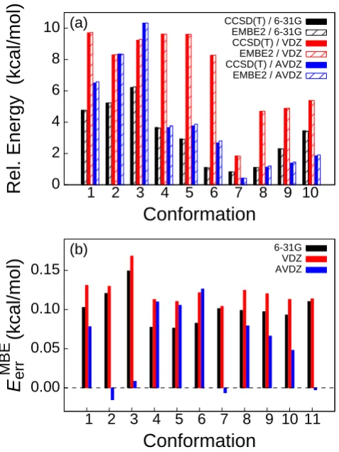
EMBE2 calculations at the CCSD(T)-in-HF level are performed on a test set of 11 conformations of the water hexamer, using the 6-31G,80,81 _{cc-pVDZ, and} aug-cc-pVDZ basis sets. The calculations are performed with {µ0, τ} = {106,0.05}, and

The relative energy of the water hexamer conformations are provided in Fig. 1.8(a), obtained using supermolecular EMBE2 calculations; full CCSD(T) calcula-tions are also reported for comparison. Energies are reported with respect to that of Conf. (11), obtained using the corresponding level of theory and basis set. Fig. 1.8(b) presents the MBE error for each calculation, obtained using

E_errMBE ≡EEMBE2−Ecorr. (1.24)

The mean unsigned MBE error, |E_errMBE|

, of the EMBE2 calculations performed on this test set is 0.10 kcal/mol for the 6-31G basis set, 0.12 kcal/mol for the cc-pVDZ basis set, and 0.06 kcal/mol for aug-cc-pVDZ. The EMBE2 calculations are thus seen to produce smaller values of

|EMBE err |

than similar calculations using point-charge embedding;67 _{equally important, however, is the fact that the embedding approach} provided here rigorously avoids the problem of charge leakage and the use of arbitrary parameters, and allows for full basis set convergence.

Fig. 1.9 presents the relative energies for the corresponding truncated embedding calculations in the aug-cc-pVDZ basis set. The border atoms are determined in the manner described in Section 1.3.2, using both RO-O = 0 ˚A (i.e., monomolecular DFT embedding using the TF KE functional) and RO-O = 3 ˚A. The truncated embedding calculations with RO-O = 3 ˚A are in far better agreement with the reference super-molecular calculations, thus illustrating the potential of using truncated projection-based embedding to significantly improve upon the accuracy of DFT embedding with approximate KE functionals.

0 2 4 6 8 10

1 2 3 4 5 6 7 8 9 10

Rel. Energy (kcal/mol)

Conformation

(a) CCSD(T) / 6-31G

EMBE2 / 6-31G CCSD(T) / VDZ EMBE2 / VDZ CCSD(T) / AVDZ EMBE2 / AVDZ

0.00 0.05 0.10 0.15

1 2 3 4 5 6 7 8 9 10 11

E

MBE err

(kcal/mol)

Conformation

(b) 6-31G

VDZ AVDZ

0 2 4 6 8 10

1 2 3 4 5 6 7 8 9 10

Relative Energy (kcal/mol)

Conformation

Supermolecular

R_O-O = 3 Å

R_O-O = 0 Å

Figure 1.9: Energies of water hexamer conformations obtained using both CCSD(T)-in-HF supermolecular EMBE2 calculations and CCSD(T)-CCSD(T)-in-HF truncated EMBE2 calculations. The embedding calculations employ truncated embedding with a border atom cutoff of eitherRO-O= 0 ˚A or RO-O = 3 ˚A. Conformation energies are reported with respect to the corresponding calculation for Conf. 11.

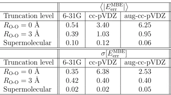
The standard deviation of the errors for each set of calculations, σ[EMBE

err ], is also provided; this quantity reports on errors in the relative conformation energies, which may be of greater practical relevance than|EMBE

err |

|EMBE err |

Truncation level 6-31G cc-pVDZ aug-cc-pVDZ

RO-O= 0 ˚A 0.54 3.40 6.25

RO-O= 3 ˚A 0.39 1.03 0.95 Supermolecular 0.10 0.12 0.06

σ[E_errMBE]

Truncation level 6-31G cc-pVDZ aug-cc-pVDZ

RO-O= 0 ˚A 0.35 6.38 2.53

RO-O= 3 ˚A 0.42 0.40 0.40 Supermolecular 0.02 0.02 0.05

Table 1.2: Summary of the EMBE2 results on the water hexamer test set. Results are listed using truncated embedding with a cutoff of RO-O = 0 ˚A, truncated embedding with a cutoff of RO-O = 3 ˚A, and supermolecular embedding. All values are in kcal/mol.

1.4.2.2 Polypeptides

EMBE2 calculations at the MP2-in-HF level are performed on several conformations of the Gly-Gly-Gly tripeptide using the cc-pVDZ and aug-cc-pVDZ basis sets. The calculations are performed with{µ0, τ}={106_{,0.05}, andv}A

NAKP[γA, γB 00

] is obtained using the TF functional. The geometries are obtained via optimization at the HF/cc-pVDZ level, with the Gly1-Gly2 bond dihedral (Ω) constrained to several values, and with all other backbone dihedral angles constrained to 180◦. Several of these geometries are shown at left in Fig. 1.10. Each monomer in the EMBE2 calculations corresponds to a set of active atoms comprised of one of the tripeptide residues. The sets of border atoms employed in the EMBE2 calculations are defined in terms of the nt cutoff, as described in Section 1.4.1.

GGG,
Ω=0°


GGG,
Ω=90°


GGG,
Ω=180°


VPL


YPY


Figure 1.10: Three of the Gly-Gly-Gly (GGG) tripeptide conformations are presented on the left for several different dihedral angles. The geometries of the Val-Pro-Leu (YPL) and Tyr-Pro-Tyr (YPY) tripeptides are presented on the right.

border atoms. Table 1.3 lists the corresponding values of |EMBE err |

and σ[EMBE err ]. In agreement with the results in Fig. 1.7, sets of border atoms associated with nt≥2 are needed to achieve suitable accuracy with the aug-cc-pVDZ basis set. Both |E_errMBE| andσ[E_errMBE] are generally found to improve with increasing numbers of border atoms. These results demonstrate that truncated EMBE2 calculations yield accurate results for systems in which embedding is performed across covalently bound monomers. Furthermore, since Ω is associated with rotation of a bond that connects different monomers, these results indicate that the EMBE2 calculations are relatively robust with respect to changes in the electronic environment in the inter-subsystem covalent bonds.

-1.5 -1.0 -0.5 0.0

0 50 100 150

Rel.

E

corr

(kcal/mol)

Ω

(Degrees)

MP2

EMBE2/Super. EMBE2/n_t = 1 EMBE2/n_t = 2 EMBE2/n_t = 3

-1.5 -1.0 -0.5 0.0

0 50 100 150

Rel.

E

corr

(kcal/mol)

Ω

(Degrees)

MP2

EMBE2/Super. EMBE2/n_t = 2 EMBE2/n_t = 3 EMBE2/n_t = 4

|EMBE err |

Basis nt= 1 nt= 2 nt = 3 nt= 4 Super. VDZ 0.106 0.345 0.103 0.007 0.050 AVDZ 18.549 0.678 0.216 0.054 0.056

σ[EMBE err ]

Basis nt= 1 nt= 2 nt = 3 nt= 4 Super. VDZ 0.112 0.033 0.028 0.008 0.002 AVDZ 19.148 0.167 0.080 0.026 0.005

Table 1.3: Summary of the EMBE2 results for the Gly-Gly-Gly tripeptide. All calcu-lations use either the cc-pVDZ (VDZ) basis set or the aug-cc-pVDZ (AVDZ) basis set. Results are provided for several values ofnt, as well as for the supermolecular basis set (Super.). Both the mean unsigned MBE error over all values of Ω and the standard deviation of the MBE error are provided. All values are reported in kcal/mol.

(Fig. 1.10, right).83,84 _{For the truncated embedding calculations, the atoms of} side-chain moieties are only included in the set of border atoms if all backbone atoms to which the side-chain moieties are bonded are border atoms.

Table 1.4 presents the results of EMBE2 calculations for the Val-Pro-Leu and Tyr-Pro-Tyr tripeptides, as well as for the Gly-Gly-Gly-Gly tetrapeptide from Section 1.4.1. Due to the computational cost of the reference calculations, results employing the aug-cc-pVDZ basis set are not included for these more complex tripeptides. As with the Gly-Gly-Gly tripeptide calculations (Fig. 1.11 and Table 1.3), the results yield small (sub kcal/mol) errors that systematically decrease with the number of border atoms.

Peptide/Basis nt= 1 nt= 2 nt = 3 nt= 4 Super. VPL/VDZ -0.029 -1.041 -0.413 -0.205 0.037 YPY/VDZ 0.604 -0.767 -0.092 -0.277 0.076 GGGG/VDZ -0.175 -0.821 -0.751 -0.066 0.095 GGGG/AVDZ 26.439 -1.513 -1.118 -0.234 0.108

1.5

Conclusions

1.6

Appendix: Water Hexamer Conformations

geometries are reported in units of ˚Angstr¨oms.

Conf. 1

O -0.01444 -1.40688 0.86698

H -0.82663 -1.49669 0.34972

H -0.12523 -1.87516 1.68772

O 0.00588 1.34004 0.84909

H 0.08181 0.39642 1.02379

H 0.79287 1.61382 0.36582

O 2.39229 -1.33294 -0.43486

H 1.59349 -1.47091 0.08523

H 2.24183 -1.68508 -1.30567

O 2.39226 1.39375 -0.42232

H 2.55075 0.44513 -0.49263

H 3.12911 1.78535 0.03323

O -2.40639 -1.30367 -0.41807

H -2.58996 -0.35940 -0.32660

H -2.41112 -1.51135 -1.34633

O -2.36824 1.39716 -0.44640

H -1.47660 1.53891 -0.10056

Conf. 2

O 0.67982 1.66847 0.22469

H 1.54472 1.23557 0.26190

H 0.80199 2.60883 0.28673

O -0.92115 -0.00176 1.65020

H -0.44806 0.77331 1.33150

H -1.76238 -0.05171 1.18135

O 0.63241 -1.64984 0.20904

H 0.08923 -1.22268 0.89198

H 0.53282 -2.59214 0.27953

O -0.42478 0.02956 -1.62376

H -0.09616 0.81284 -1.17004

H 0.00023 -0.73782 -1.22438

O 2.74478 -0.02765 -0.08537

H 2.20281 -0.78880 0.15326

H 2.94467 -0.09143 -1.01363

O -2.76330 -0.07803 -0.30968

H -2.08455 -0.14812 -0.99436

Conf. 3

O 1.38240 -0.79588 1.21410

H 0.45622 -0.77606 1.50601

H 1.91210 -1.20090 1.89061

O 1.48104 1.37700 -0.30523

H 1.66217 0.81313 0.45827

H 2.14568 2.05442 -0.35742

O 1.06670 -1.01572 -1.39720

H 1.28587 -1.35829 -0.52354

H 1.27925 -0.07519 -1.39115

O -1.27339 -0.50500 1.53311

H -1.33645 0.44562 1.36259

H -1.58576 -0.94802 0.73654

O -1.20461 1.67808 0.04663

H -0.27064 1.81552 -0.13712

H -1.54482 1.05338 -0.60204

O -1.58571 -0.71089 -1.07832

H -0.70068 -0.95230 -1.38904

Conf. 4

O 18.0712 -51.4753 1.0577

H 18.3158 -52.4080 1.0702

H 18.9200 -50.9885 0.9316

O 20.4013 -50.1151 0.6787

H 20.3203 -49.3282 0.0893

H 20.8628 -49.7855 1.4593

O 20.1820 -47.9418 -0.9528

H 19.3727 -47.3927 -0.8299

H 20.2353 -48.1019 -1.9024

O 15.8359 -50.5064 -0.1649

H 15.7879 -50.8915 -1.0479

H 16.6469 -50.8938 0.2396

O 17.9552 -46.4504 -0.4572

H 17.7010 -45.6711 -0.9652

H 17.1102 -46.9274 -0.2792

O 15.6330 -47.7931 0.0179

H 15.7046 -48.7745 -0.0499

Conf. 5

O 26.0243 -46.8132 0.6983

H 25.9101 -46.6716 1.6460

H 26.0029 -47.7919 0.5870

O 26.0716 -49.5194 0.3763

H 26.7867 -49.9034 -0.1830

H 25.3029 -50.0816 0.2267

O 28.1035 -50.5775 -1.1078

H 29.0003 -50.2744 -0.8287

H 28.1161 -50.5173 -2.0704

O 28.2510 -45.6677 -0.3766

H 27.9994 -45.4294 -1.2768

H 27.4402 -46.0768 0.0100

O 30.5786 -49.7113 -0.3571

H 30.9359 -50.1242 0.4385

H 30.6024 -48.7444 -0.1688

O 30.5444 -47.0387 0.1802

H 29.7277 -46.5346 -0.0448

Conf. 6

O -0.1141 -45.4756 0.4357

H -0.1212 -45.0081 1.2795

H -0.9900 -45.9275 0.3939

O -2.6533 -49.4119 0.4391

H -1.8471 -49.9163 0.1772

H -2.9576 -49.8399 1.2483

O 2.1002 -46.9006 -0.2471

H 2.4044 -46.4744 -1.0573

H 1.2956 -46.3941 0.0156

O -0.4370 -50.8340 -0.2436

H 0.4396 -50.3836 -0.2009

H -0.4308 -51.2999 -1.0883

O 1.9963 -49.6175 -0.1859

H 2.6080 -49.8611 0.5191

H 2.0244 -48.6317 -0.2130

O -2.5466 -46.6945 0.3830

H -3.1568 -46.4524 -0.3238

Conf. 7

O 10.1313 -39.6546 -1.2837

H 10.9834 -39.2940 -0.9427

H 10.3710 -40.2693 -1.9876

O 8.5206 -37.2415 -1.1214

H 8.9694 -38.0370 -1.4609

H 7.6674 -37.5876 -0.7864

O 10.0161 -37.0305 1.0891

H 9.4323 -36.9616 0.2835

H 9.9503 -36.1767 1.5337

O 8.7588 -39.6895 1.2947

H 9.2025 -39.9141 0.4565

H 9.1929 -38.8551 1.5467

O 12.1674 -38.3372 -0.0356

H 11.5483 -37.7652 0.4699

H 12.7194 -38.7610 0.6334

O 6.4748 -38.4556 0.3410

H 7.1523 -39.0355 0.7568

Conf. 8

O 15.9468 -39.5823 0.5548

H 15.3045 -40.0871 0.0416

H 16.8221 -39.7683 0.1280

O 18.3471 -39.7460 -0.6662

H 19.1305 -40.0034 -0.1359

H 18.5029 -38.8042 -0.8557

O 20.6467 -40.0714 0.9070

H 21.4549 -40.4532 0.5435

H 20.8337 -39.1110 0.9827

O 20.8368 -37.2970 0.9070

H 20.0333 -37.0136 0.4221

H 20.8440 -36.7677 1.7135

O 16.1147 -36.8858 0.5596

H 15.9307 -37.8581 0.5885

H 15.9523 -36.5744 1.4583

O 18.5450 -36.8241 -0.6030

H 18.5146 -36.2064 -1.3439

Conf. 9

O 29.7954 -37.1884 -0.3910

H 30.6865 -36.9230 -0.1328

H 29.8886 -38.1244 -0.7014

O 29.8265 -39.8168 -1.0122

H 29.6466 -40.1441 -1.9019

H 29.0506 -40.1097 -0.4687

O 27.7083 -40.3069 0.6051

H 27.6403 -39.4409 1.0439

H 26.8649 -40.3743 0.1095

O 25.3507 -40.1183 -0.9006

H 24.5083 -40.4902 -0.6120

H 25.2501 -39.1476 -0.7875

O 25.3917 -37.3962 -0.3791

H 25.5108 -36.7584 -1.0937

H 26.1882 -37.2944 0.1837

O 27.6626 -37.4465 1.2384

H 27.7398 -36.9721 2.0750

Conf. 10

O 7.5344 -47.1952 0.4765

H 8.4160 -47.2312 0.0120

H 7.2660 -46.2693 0.4279

O 8.1630 -50.9274 0.5473

H 8.2441 -50.4060 1.3688

H 7.3554 -50.5591 0.1389

O 9.8927 -47.4450 -0.7542

H 10.6734 -47.2098 -0.2369

H 10.0133 -48.4102 -0.9487

O 10.1564 -50.1025 -1.0813

H 10.0613 -50.5472 -1.9320

H 9.4474 -50.4883 -0.5041

O 8.2958 -48.9198 2.5834

H 7.7974 -48.8686 3.4078

H 7.9420 -48.2014 2.0231

O 6.1151 -49.3715 -0.6444

H 6.4601 -48.5223 -0.3019

Conf. 11

O -1.9241 -39.9369 0.2244

H -1.7339 -40.0619 -0.7214

H -2.0308 -38.9602 0.2590

O -1.6252 -37.1872 -0.1835

H -1.3632 -37.4801 -1.0740

H -0.7751 -37.0474 0.2718

O -0.7346 -39.0353 -2.2858

H -0.6724 -39.1225 -3.2446

H 0.1927 -39.1034 -1.9556

O 1.6853 -39.1868 -1.0050

H 1.7953 -38.3281 -0.5647

H 1.4640 -39.7654 -0.2520

O 0.4498 -40.0965 1.4209

H -0.4725 -40.1381 1.0403

H 0.4880 -40.7832 2.0974

O 0.9394 -37.3782 1.1917

H 1.2480 -36.8472 1.9361

1.7

Appendix: Gly-Gly-Gly Tripeptide

Conformations

The value of Ω is provided for each conformation. All geometries are reported in units of ˚Angstr¨oms.

Ω = 0

Ω = 15

Ω = 30

Ω = 45

Ω = 60

Ω = 75

Ω = 90

Ω = 105

Ω = 120

Ω = 135

Ω = 150

Ω = 165

Ω = 180

1.8

Appendix: Additional Polypeptides

Gly-Gly-Gly-Gly Tetrapeptide

Val-Pro-Leu Tripeptide

Tyr-Pro-Tyr Tripeptide

Bibliography

[1] A. Warshel and M. Levitt, J. Mol. Biol. 103, 227 (1976).

[2] P. Sherwood, A. H. de Vries, S. J. Collins, S. P. Greatbanks, N. A. Burton, M. A. Vincent, and I. H. Hillier, Faraday Discuss. 106, 79 (1997).

[3] J. L. Gao, P. Amara, C. Alhambra, and M. J. Field, J. Phys. Chem. A 102, 4714 (1998).

[4] H. Lin and D. G. Truhlar, Theor. Chem. Acc. 117, 185 (2007).

[5] H. M. Senn and W. Thiel, Angew. Chem., Int. Ed.48, 1198 (2009).

[6] L. Hu, P. S¨oderhjelm, and U. Ryde, J. Chem. Theory Comput. 7, 761 (2011).

[7] S. Dapprich, I. Kom´aromi, K. S. Byun, K. Morokuma, and M. J. Frisch, THEOCHEM 461-462, 1 (1999).

[8] F. Maseras and K. Morokuma, J. Comp. Chem. 16, 1170 (1995).

[9] K. Kitaura, E. Ikeo, T. Asada, T. Nakano, and M. Uebayasi, Chem. Phys. Lett.

313, 701 (1999).

[10] D. G. Federov and K. Kitaura, J. Chem. Phys.120, 6832 (2004).

[11] D. G. Federov and K. Kitaura, J. Phys. Chem. A111, 6904 (2007).

[13] S. R. Pruitt, M. A. Addicoat, M. A. Collins, and M. S. Gordon, Phys. Chem. Chem. Phys. 14, 7752 (2012).

[14] K. R. Brorsen, N. Minezawa, F. Xu, T. L. Windus, and M. S. Gordon, J. Chem. Theory Comput. 8, 5008 (2012).

[15] A. Gaenko, T. L. Windus, M. Sosonkina, and M. S. Gordon, J. Chem. Theory Comput. 9, 222 (2013).

[16] N. Govind, Y. A. Yang, A. J. R. da Silva, and E. A. Carter, Chem. Phys. Lett.

295, 129 (1998).

[17] N. Govind, Y. A. Wang, and E. A. Carter, Phys. Rev. B 110, 7677 (1999).

[18] T. Kl¨uner, N. Govind, Y. A. Yang, and E. A. Carter, J. Chem. Phys. 116, 42 (2002).

[19] P. Huang and E. A. Carter, J. Chem. Phys. 125, 084102 (2006).

[20] S. Sharifzadeh, P. Huang, and E. Carter, J. Phys. Chem. C 112, 4649 (2008).

[21] A. S. P. Gomes, C. R. Jacob, and L. Visscher, Phys. Chem. Chem. Phys. 10, 5353 (2008).

[22] T. A. Wesolowski, Phys. Rev. A 77, 012504 (2008).

[23] Y. G. Khait and M. R. Hoffmann, J. Chem. Phys. 133, 044107 (2010).

[24] C. Huang, M. Pavone, and E. A. Carter, J. Chem. Phys.134, 154110 (2011).

[25] C. Huang and E. A. Carter, J. Chem. Phys. 135, 194104 (2011).

[26] S. Hofener, A. S. P. Gomes, and L. Visscher, J. Chem. Phys.136, 044104 (2012).

[28] A. Severo Pereira Gomes and C. R. Jacob, Annu. Rep. Prog. Chem., Sect. C: Phys. Chem. 108, 222 (2012).

[29] J. D. Goodpaster, T. A. Barnes, F. R. Manby, and T. F. Miller III, J. Chem. Phys. 137, 224113 (2012).

[30] F. R. Manby, M. Stella, J. D. Goodpaster, and T. F. Miller III, J. Chem. Theory Comput. 8, 2564 (2012).

[31] J. D. Goodpaster, N. Ananth, F. R. Manby, and T. F. Miller III, J. Chem. Phys.

133, 084103 (2010).

[32] J. D. Goodpaster, T. A. Barnes, and T. F. Miller III, J. Chem. Phys. 134, 164108 (2011).

[33] S. Fux, C. R. Jacob, J. Neugebauer, L. Visscher, and M. Reiher, J. Chem. Phys.

132, 164101 (2010).

[34] J. Nafziger, Q. Wu, and A. Wasserman, J. Chem. Phys. 135, 234101 (2011).

[35] P. D. Ded´ıkov´a, P. Neogr´ady, and M. Urban, J. Phys. Chem. A115, 2350 (2011).

[36] P. G. Lykos and R. G. Parr, J. Chem. Phys. 24, 1166 (1956).

[37] J. C. Phillips and L. Kleinman, Phys. Rev.116, 287 (1959).

[38] H. Stoll, B. Paulus, and P. Fulde, J. Chem. Phys. 123, 144108 (2005).

[39] R. A. Mata, H.-J. Werner, and M. Sch¨utz, J. Chem. Phys.128, 144106 (2008).

[40] T. M. Henderson, J. Chem. Phys. 125, 014105 (2006).

[41] A. A. Cantu and S. Huzinaga, J. Chem. Phys.55, 5543 (1971).

[43] J. L. Pascual, N. Barros, Z. Barandiaran, and L. Seijo, J. Phys. Chem. A 113, 12454 (2009).

[44] H.-J Werner, P. J. Knowles, R. Lindh, F. R. Manby, M. Sh¨utz et al., MOLPRO, version 2008.3, a package of ab initio programs, 2008, see www.molpro.net. [45] B. Temelso, K. A. Archer, and G. C. Shields, J. Phys. Chem. A 115, 12034

(2011).

[46] T. H. Dunning, Jr., J. Chem. Phys. 90, 1007 (1989).

[47] R. A. Kendall, T. H. Dunning, and R. J. Harrison, J. Chem. Phys. 96, 6796 (1992).

[48] J. Pipek and P. Mezey, J. Chem. Phys. 90, 4916 (1989).

[49] K. Raghavachari, G. W. Trucks, J. A. Pople, and M. Head-Gordon, Chem. Phys. Lett. 157, 479 (1989).

[50] E. V. Stefanovich and T. N. Truong, J. Chem. Phys. 104, 2946 (1996).

[51] A. Laio, J. VandeVondele, and U. Rothlisberger, J. Chem. Phys. 116, 6941 (2002).

[52] K. Senthilkumar, J. I. Mujika, K. E. Ranaghan, F. R. Manby, A. J. Mulholland, and J. N. Harvey, J. R. Soc. Interface 5, S207 (2008).

[53] L. H. Thomas, Proc. Cambridge Philos. Soc. 23, 542 (1927).

[54] E. Fermi, Z. Phys. 48, 73 (1928).

[55] C. R. Jacob, T. A. Wesolowski, and L. Visscher, J. Chem. Phys. 123, 174104 (2005).

[57] C. R. Jacob, S. M. Beyhan, and L. Visscher, J. Chem. Phys.126, 234116 (2007).

[58] E. Dahlke and D. Truhlar, J. Phys. Chem. B 110, 10595 (2006).

[59] S. Hirata, O. Sode, M. Ke¸celi, and T. Shimazaki, Accurate Condensed Phase

Quantum Chemistry (Taylor and Francis, 2011).

[60] P. J. Bygrave, N. L. Allan, and F. R. Manby, J. Chem. Phys. 137, 164102 (2012).

[61] C. R. Taylor, P. J. Bygrave, J. N. Hart, N. L. Allan, and F. R. Manby, Phys. Chem. Chem. Phys. 14, 7739 (2012).

[62] E. E. Dahlke and D. G. Truhlar, J. Chem. Theory Comput. 3, 46 (2007).

[63] E. E. Dahlke and D. G. Truhlar, J. Chem. Theory Comput. 3, 1342 (2007).

[64] H. Lin and D. G. Truhlar, Theor. Chem. Acc. 117, 185 (2007).

[65] E. E. Dahlke and D. G. Truhlar, J. Chem. Theory Comput. 4, 1 (2008).

[66] A. Sorkin, E. E. Dahlke, and D. G. Truhlar, J. Chem. Theory Comput. 4, 683 (2008).

[67] E. E. Dahlke, H. R. Leverentz, and D. G. Truhlar, J. Chem. Theory Comput.

4, 33 (2008).

[68] L. D. Jacobson and J. M. Herbert, J. Chem. Phys. 134, 094118 (2011).

[69] S. Hirata, Chem. Phys. Phys. Chem. 11, 8397 (2009).

[70] R. M. Richard and J. M. Herbert, J. Chem. Phys. 137, 064113 (2012).

[72] S. Wen, K. Nanda, Y. Huang, and G. J. O. Beran, Phys. Chem. Chem. Phys.

14, 7578 (2012).

[73] E. B. Kadossov, K. J. Gaskell, and M. A. Langell, J. Comput. Chem. 28, 1240 (2007).

[74] U. C. Deev and P. A. Kollman, J. Comput. Chem. 7, 718 (1986).

[75] M. J. Field, P. A. Bash, and M. Karplus, J. Comput. Chem. 11, 700 (1990).

[76] V. Deev and M. A. Collins, J. Chem. Phys. 122, 154102 (2005).

[77] M. A. Collins and V. A. Deev, J. Chem. Phys. 125, 104104 (2006).

[78] D. W. Zhang, X. H. Chen, and J. Z. H. Zhang, J. Comput. Chem. 24, 1846 (2003).

[79] D. W. Zhang and J. Z. H. Zhang, J. Chem. Phys. 119, 3599 (2003).

[80] R. Ditchfield, W. J. Hehre, and J. A. Pople, J. Chem. Phys. 54, 724 (1971).

[81] W. J. Hehre, R. Ditchfield, and J. A. Pople, J. Chem. Phys. 56, 2257 (1972).

[82] M. D. Tissandier, S. J. Singer, and J. V. Coe, J. Phys. Chem. A104, 752 (2000).

[83] S. C. Graham and J. M. Guss, Arch. Biochem. Biophys. 469, 200 (2008).

Chapter 2

Ab initio

characterization of the

electrochemical stability and

solvation properties of

condensed-phase ethylene

carbonate and dimethyl carbonate

mixtures

2.1

Introduction

The commercial market for Li-ion batteries is currently dominated by cells that utilize carbonate-based electrolytes and have cathodes that operate at potentials in the range of 3.5-4.2 V vs. Li.1–6 Higher operational voltages would enable Li-ion batteries with greater energy density. However, typical carbonate solvents in these batteries undergo oxidation by the charged cathode surface at voltages exceeding 4.5 V vs. Li.5 Following oxidation, the solvent molecules further decompose via pathways that have been implicated in capacity fade upon cycling.2,5,7–12

stability on high voltage cathodes.10,16,17 _{Similarly, ionic liquids have attracted} con-siderable interest due to their high electrochemical stability.18–20 _{Unfortunately, these} alternatives to traditional carbonate-based solvents typically suffer from other prob-lems, such as high viscosity or the inability to form a robust solid electolyte interphase (SEI).17

A central obstacle in the pursuit of expanded windows of electrochemical stability is elucidation of the mechanisms by which each electrolyte component influences the oxidation potential of the other components. For example, the oxidation potentials of carbonate solvents are known to be influenced by the presence of co-solvents2 _and solvated ions,21–23_{as well as by the electrode composition.}24,25_{This makes} experimen-tal investigation of oxidation potentials challenging, since all of these factors must be considered.

To complement these experimental efforts, theoretical studies have attempted to identify the intrinsic oxidation potential of the individual components of battery elec-trolytes. The intrinsic oxidation potential corresponds to the oxidation potential of each electrolyte component in the absence of an electrode and any oxidation-inducing decomposition reactions. The majority of these theoretical studies have been con-ducted using DFT methods10,11,19–21,23,26–40 _{or WFT methods}10,27,41–43 _{applied in} ei-ther the gas phase26,27,35 or using implicit solvation models.10,11,27,31–39,41,42 Only a few studies on electrolytes have utilized an explicit representation of the environ-ment; these include QM/MM calculations on large clusters,20 _{and condensed-phase} calculations using DFT with periodic boundary conditions.19,23,30,40

condensed-(a)
 (b)


Ac(ve
 DFT
 MM


Figure 2.1: Summary of the embedding protocol. (a) MD simulations are performed to generate the equilibrium ensemble of solvent configurations. (b) An embedded CCSD(T) calculation is performed on a single molecule from the MD simulation (the “active region”), indicated by the red circle. The electron hole created upon oxidation of the active region is illustrated by the blue electron cloud. Nearby molecules are treated at the B3LYP level,47,48 _{indicated by the blue circle. More distant molecules} are treated using a point-charge molecular-mechanics (MM) model, indicated by the brown circle.

phase systems, we examine the effect of intermolecular interactions on the vertical IE of individual solvent molecules, and find that conventional implicit solvent mod-els neglect interactions that are necessary to understand the electrochemistry and solvation properties of DMC. These observations enable a simple and intuitive ex-planation for experimentally-observed anomalies in the solvation structure of ions in carbonate-based electrolytes.

2.2

WFT-in-DFT Embedding for Condensed-Phase

Systems

2.2.1

Overview of Embedding Strategy

Fig. 2.1 illustrates the overall embedding strategy employed for calculation of the oxidation potentials of EC and DMC mixtures, which consists of three main steps. The following is a brief overview of each step: