Learning by observation through system identification

This is a repository copy of

Learning by observation through system identification

.

White Rose Research Online URL for this paper:

http://eprints.whiterose.ac.uk/74610/

Monograph:

Nehmzow, U., Akanyeti, O., Weinrich, C. et al. (2 more authors) (2007) Learning by

observation through system identification. Research Report. ACSE Research Report no.

952 . Automatic Control and Systems Engineering, University of Sheffield

[email protected] https://eprints.whiterose.ac.uk/

Reuse

Unless indicated otherwise, fulltext items are protected by copyright with all rights reserved. The copyright exception in section 29 of the Copyright, Designs and Patents Act 1988 allows the making of a single copy solely for the purpose of non-commercial research or private study within the limits of fair dealing. The publisher or other rights-holder may allow further reproduction and re-use of this version - refer to the White Rose Research Online record for this item. Where records identify the publisher as the copyright holder, users can verify any specific terms of use on the publisher’s website.

Takedown

If you consider content in White Rose Research Online to be in breach of UK law, please notify us by

Learning by Observation through System Identification

U Nehmzow

, O. Akanyeti

, C Weinrich

, T Kyriacou

, S A Billings

#Dept Computer Science, University of Essex

Department of Automatic Control and Systems Engineering

The University of Sheffield, Sheffield, S1 3JD, UK

Research Report No. 952

Learning by Observation through System

Identification

Ulrich Nehmzow

, Otar Akanyeti

, Cristoph Weinrich

, Theocharis Kyriacou

,

Steve Billings

1

_{Dept. of Computer Science, University of Essex, UK.}

2

_{Dept. of Automatic Control and Systems Engineering, University of Sheffield, UK.}

Abstract

In our previous works, we present a new method to program mobile robots —“code identification by demonstration”— based on algorithmically transfer-ring human behaviours to robot control code using transparent mathematical functions. Our approach has three stages: i) first extracting the trajectory of the desired behaviour by observing the human, ii) mak-ing the robot follow the human trajectory blindly to log the robot’s own perception perceived along that trajectory, and finally iii) linking the robot’s percep-tion to the desired behaviour to obtain a generalised, sensor-based model.

So far we used an external, camera based motion tracking system to log the trajectory of the human demonstrator during his initial demonstration of the desired motion. Because such tracking systems are complicated to set up and expensive, we propose an alternative method to obtain trajectory information, using the robot’s own sensor perception.

In this method, we train a mathematical polynomial using the NARMAX system identification method-ology which maps the position of the “red jacket” worn by the demonstrator in the image captured by the robot’s camera, to the relative position of the demon-strator in the real world according to the robot.

We demonstrate the viability of this approach by teaching a Scitos G5 mobile robot to achieve door traversal behaviour.

1.

Introduction

Increasingly, personalised robots — robots especially de-signed and programmed for an individual’s needs and pref-erences — are being used to support humans in their daily lives, most notably in the area of service robotics. Arguably, the closer the robot is programmed to the individual’s needs, the more useful it is, and we believe that giving people the op-portunity to program their own robots, rather than program-ming robots for them, will push robotics research one step further in the personalised robotics field.

However, traditional robot programming techniques — besides being costly, time-consuming and error prone (Iglesias et al., 2005) — require specialised technical skills from different disciplines and it is not reasonable to expect end-users to have these skills.

In (Nehmzow et al., 2007) and (Akanyeti et al., 2007b) we presented a novel method to translate human behaviours into robot control code algorithmically, using system iden-tification techniques such as Armax (Auto-Regressive Mov-ing Average models with eXogenous inputs) (Eykhoff, 1974) and Narmax (Nonlinear Armax) (Billings and Chen, 1998). These techniques produce linear or nonlinear polynomial functions that model the relationship between the robot’s sen-sor perception and motor response.

Our method has three stages: i) The human operator demonstrates the desired behaviour to the robot. ii) the robot imitates the desired behaviour blindly (i.e.without us-ing sensor perception), usus-ing recursive, sensor-free poly-nomials. During this first run through the task the robot logs perception-action data to obtain a sensor-based con-trol model, and iii) using the logged data, we obtain a sensor-based controller, using transparent mathematical func-tions which capture the fundamental relafunc-tionship between the robot’s perception and the desired motor response.

During the human user’s initial demonstration of the de-sired motion, so far we used an external, camera based mo-tion tracking system to log the trajectory informamo-tion. Such tracking systems are complicated to set up and we can not expect the end users who want to program their own robots would have this kind of expensive facility in their houses.

In this paper, we therefore propose a new method replacing the Vicon motion tracking system with the Narmax polyno-mial models which are trained to predict the position of the demonstrator using the robot’s own vision system.

2.

Methodology and Experimental Setup

2.1

Narmax system identification methodology

For multiple input, single output noiseless systems this model takes the form of equation 1. A detailed discussions can be found in (Billings and Chen, 1998), (Korenberg et al., 1988, Billings and Voon, 1986).

y(n) = f(u1(n),u1(n−1),u1(n−2),· · ·,u1(n−Nu), (1)

u1(n)2,u1(n−1)2,u1(n−2)2,· · ·,u1(n−Nu)2,

· · ·,

u1(n)l,u1(n−1)l,u1(n−2)l,· · ·,u1(n−Nu)l,

u2(n),u2(n−1),u2(n−2),· · ·,u2(n−Nu),

u2(n)2,u2(n−1)2,u2(n−2)2,· · ·,u2(n−Nu)2,

· · ·,

u2(n)l,u2(n−1)l,u2(n−2)l,· · ·,u2(n−Nu)l,

· · ·,

ud(n),ud(n−1),ud(n−2),· · ·,ud(n−Nu),

ud(n)2,ud(n−1)2,ud(n−2)2,· · ·,ud(n−Nu)2,

· · ·,

ud(n)l,ud(n−1)l,ud(n−2)l,· · ·,ud(n−Nu)l,

y(n−1),y(n−2),· · ·,y(n−Ny),

y(n−1)2_,y(n−2)2_{,· · ·,y(n−N} y)2, · · ·,

y(n−1)l_,y(n−2)l_{,· · ·,y(n−N} y)l)

y(n) and u(n) are the sampled output and input signals at time n respectively, Ny and Nu are the regression orders

of the output and input respectively, d is the dimension of the input vector and l is the degree of the polynomial. f()

is a non-linear function and here taken to be a polynomial multi-resolution expansion of its arguments. Expansions such as multi-resolution wavelets or Bernstein coefficients can be used as an alternative to the polynomial expansions consid-ered in this study.

The representation of the task as a transparent, analysable model enables us to investigate the various factors that affect robot behaviour for the task at hand. For in-stance, we can identify input-output relationships such as the sensitivity of a robot’s behaviour to particular sensors (Roberto Iglesias and Billings, 2005), or make predictions of behaviour when a particular input is presented to the robot (Akanyeti et al., 2007a).

2.2

Learning by Observation

Human demonstration First, the human user demonstrates the desired behaviour by performing it in the target environ-ment. For the purpose of this paper we confined our ex-periments to 2-dimensional navigation problems due to the limited motion capabilities of our robot (2 degrees of mo-tion, translational and rotational, figure 1). During this initial demonstration, we log thexandyposition of the human user using the motion tracking system. Once the operator’s tra-jectory is logged, we compute the translational and rotational velocities of the human by using consecutive (x,y) samples along the trajectory.

Sensorless trajectory following In a second stage, we use the Narmax system identification method to obtain two

sensor-free polynomials, one expressing rotational velocity as a function of time and past rotational velocities, the other expressing the translational velocity as a function of time and past linear velocities. We then use these two sensor-free poly-nomials to drive the robot along the trajectory the human had taken earlier, now logging sensor readings and velocities.

Obtaining the final, sensor-based controllers The sensor-free controllers obtained at stage II are essentially ballistic controllers that drive the robot along the desired trajectory as long as the robot is started from the same initial positions as the human. However, for real-world applications it is essen-tial that sensor feedback is used to control the motion of the robot.

In the final stage we therefore use the Narmax system iden-tification method to obtain sensor-based controllers, using the previously logged sensor-motor pairings. This controller can subsequently be used to control the robot in the target en-vironment, copying the original behaviour exhibited by the human demonstrator.

2.3

Experimental Setup

The experiments described in this paper were conducted in the 100 square meter circular robotics arena of the University of Essex. The arena is equipped with a Vicon motion tracking system which can deliver position data (x,yandz) for the full range of targets using reflective markers and high speed, high resolution cameras. The tracking system is capable of sam-pling the motion upto 100Hz within a 10mm range accuracy. We used a Scitos G5 mobile robot called REX(figure 1).

The robot is equipped with a ring of 24 sonar and 24 infra-red sensors, both uniformly distributed. A Hokuyo laser range finder is also present on the front part of the robot. This range sensor has a wide angular range (240 degree) with a radial resolution of 0.36 degree and distance resolution of less than 1cm . The robot also incorporates a colour video camera with 640×480 pixels resolution which can deliver colour images upto 60Hz .

3.

Human Trajectory Prediction

In this section we propose an alternative method to obtain the trajectory information of the human user during his demon-stration of the desired behaviour, using the robot’s own sensor perception rather than the Vicon motion tracking system.

3.1

Method

robot

angle 240 angle 0

laser av lv + − − u1 u2 u3 u4 u5 u6 u7 u8 u9 u11 u10 + (a) (b)

Figure 1: REX(a). RAXhas two degrees of freedom (translational and rotational) and equipped with the laser range finder. The range finder has a wide angular range (240 degree) with a radial resolution of 0.36 degree and distance resolution of less than 1cm. During experiments, in order to decrease the dimensionality of the input space to Narmax model, we coarse coded the laser readings into 11 sectors (u1tou11) by averaging 62 readings for each 22 degree intervals (b).

x

x

y

y

Narmax

human X pos.

x

x

y

y

Narmax

human Y pos.

Figure 2: Position prediction models. These models are mathemat-ical descriptions that define the relationship between the position of the jacket in the image and the relative position of the demon-strator referenced to the robot’s coordinate system. (xmin,ymin)and

(xmax,ymax)are the coordinates of the “left up” and “right down” corners of the rectangle surrounding the red jacket respectively (see figure 3 ). These coordinates are computed by separating the “red jacket” from the background of the image using a blob colouring algorithm.

x

y

y

x

X axis

Y axis

+y

−y

+x

robot’s coordinate system 0,0

(a) (b)

Figure 3: The output image after a pre processing stage (a). The demonstrator’s jacket was isolated from the rest of the image. The position of the jacket was computed using a blob colouring algo-rithm based on the image coordinate frame as shown in the figure. The position information of the jacket is then fed to Narmax poly-nomials which are trained to predict the real position of the demon-strator relative to the robot’s reference coordinate system shown in (b).

Finding the position of the jacket Figure 4 shows the block diagram that illustrates how we extract the position of the red jacket from the captured images.

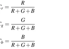
First we rectify the captured images in order to minimize the effect of distortion due to the oval shape of the camera lens. Once the image is rectified, we convert it into “chro-maticity colour space” which is less illumination dependent that the RGB colour space.

Cr= R

R+G+B (2)

Cg= G

R+G+B (3)

C_b= B

R+G+B (4)

whereCr,CgandCbare the red chromaticity, green

chro-maticity and blue chrochro-maticity components respectively, and

R,GandBare the red, green and blue values respectively of the colour to be described.

In the final stage, we separate the jacket from the back-ground of the image by using a blob colouring algorithm. Blob colouring is a technique used to find regions of simi-lar colour in the image. The connected pixels are grouped together if they have similar intensity values and assigned to different regions if the difference in their intensity values is bigger than a certain threshold.

Chromaticity space

Blob colouring

Image rectification

Raw image

the jacket

position of

x

_x

max

max min

y

y

Figure 4: The block diagram that illustrates how the position of the red jacket is extracted from the captured images. First the images are rectified in order to minimize the effect of distortion due to the oval shape of the camera lens. Once the image is rectified, it is converted into chromaticity space which is less illuminant dependent. And in the final stage, the jacket is separated from the background of the image by blob colouring algorithm (see figure 3).

the rectangle are then fed to Narmax polynomials obtained as described in section 3.2 to predict the position of the demon-strator.

3.2

Acquisition of estimation and training data

set in order to obtain Narmax polynomials

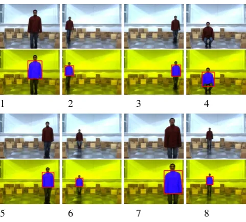
In order to collect training data for the estimation of the demonstrator’s position, the human trainer wearing a red jacket walked randomly in the robot’s field of view for half an hour. During the training session the robot was static and the robot’s camera was aligned parallel to the floor so that the robot’s field of view has the maximum coverage area for the demonstrator.

During this time the position of the jacket in the captured images and the relative position of the demonstrator refer-enced to the robot — obtained through the Vicon motion tracking system — were logged synchronously every 250ms. Figure 5 shows stream of original and the processed images captured during the training session.

3.3

Obtaining position prediction models

We then used the Narmax system identification procedure to estimate the relative position of the demonstrator referenced to the robot as a function of the position of the jacket in the image (xmin,xmax,yminandymax). TheX position prediction

model was chosen to be second degree with no regression in the input and output (i.e.l=2,Nu=0,Ny=0). The resulting

model contained 6 terms. TheY position prediction model was chosen to be fourth degree with no regression in the input and the output (i.e. l=4,Nu=0, Ny=0) and contained 7

1 2 3 4

5 6 7 8

Figure 5: Stream of images captured by the robot’s camera during the acquisition of the training data set used in obtaining Narmax model in order to calculate the relative position of the demonstrator according to the robot. Each image is pre processed using the proce-dure given in figure 4 in order to extract the position of the red jacket in the image.

terms. Both models are given in table 1.

X(n) = Y(n) =

+14.684 −4.128

+0.148∗u(n,3) −0.015∗u(n,1)

−0.184∗u(n,4) +0.051∗u(n,2)

+0.001∗u(n,3)2

−0.001∗u(n,2)2

+0.001∗u(n,4)2 _+0.001

∗u(n,1)∗u(n,2)2

−0.001∗u(n,3)∗u(n,4) +0.001∗u(n,1)∗u(n,1)3

−0.001∗u(n,1)∗u(n,2)3

Table 1: Two position polynomials which link the perception of the robot to the position of the demonstrator in the robot’s reference frame. X(n)andY(n)are thexposition (inm) and yposition (in

rad/s) of the demonstrator at time instantnandu1tou4are thexmin,

xmax,yminandymax coordinates of the “red jacket blob” extracted from the image as described in figure 4.

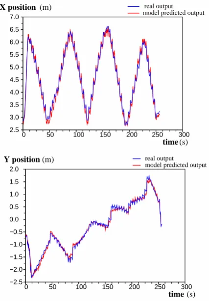
Figure 6 shows the predicted and actual position of the demonstrator in the robot’s coordinate frame.

Model validation We compared the predicted position of the demonstrator with the actual position by analysing the er-ror distributions. The results show that the average erer-ror be-tween the predicted and actual position of the demonstrator is less than 10±0.3cm for both models (see figure 7).

4.

Experiment: Door Traversal

door-X position (m)

time (s) real output

0 50 100 150 200 250 300

2.5 3.0 3.5 4.0 4.5 5.0 5.5 6.0 6.5

7.0 model predicted output

Y position (m)

time (s)

0 50 100 150 200 250 300

−2.5 −2.0 −1.5 −1.0 −0.5 0.0 0.5 1.0 1.5

2.0 model predicted output

real output

Figure 6: The predicted and actual position of the demonstrator in the robot’s coordinate frame.

X pos. prediction error (m)

frequency

−0.3 −0.2 −0.1 0.0 0.1 0.2 0.3 0.4

0.0 0.5 1.0 1.5 2.0 2.5 3.0 3.5 4.0 4.5 5.0

0.009m 0.113 mean = std. dev =

Y pos. prediction error (m)

frequency

−0.4 −0.3 −0.2 −0.1 0.0 0.1 0.2 0.3

0 5

4

3

2

1 6 7 8 9

mean = std. dev. = 0.080

0.008m

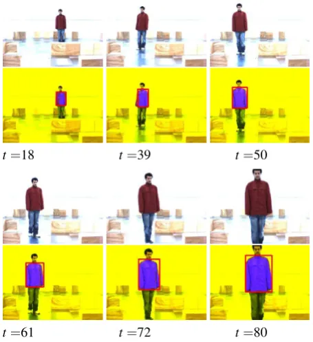
traversal behaviour. The demonstrator walked through two consecutive door like openings of 120cm width. During this time, the robot calculates the trajectory of the demonstrator using the trajectory capturing mechanism described in sec-tion 3. every 250ms. Figure 8 shows the general experimental scenario in which the demonstrator performed the desired be-haviour while the robot was observing him. Figure 9 shows the stream of images which were captured and processed by the robot during the demonstration.

REX HUMAN

Figure 8: The trajectory followed by the demonstrator while pass-ing through the two door like openpass-ings of 120cm width. While the demonstrator was performing the desired behaviour, the robot was observing him and calculating the demonstrator’s relative trajectory according to the robot itself using position prediction models given in table 2.

Analysis of the observed trajectory reveals that there is noise in the data because of two reasons:

1. There is a constant oscillation in the motion of the demon-strator, which originates from the swinging motion per-pendicular to the heading direction. This is a general char-acteristic of the two legged locomotion in humans.

2. The polynomials that compute the position of the demon-strator reference to the robot are extremely sensitive to how accurate the position of the jacket is extracted from the image. The blob colouring algorithm is not a very ro-bust method of image segmentation in the environments where the illumination is variant.

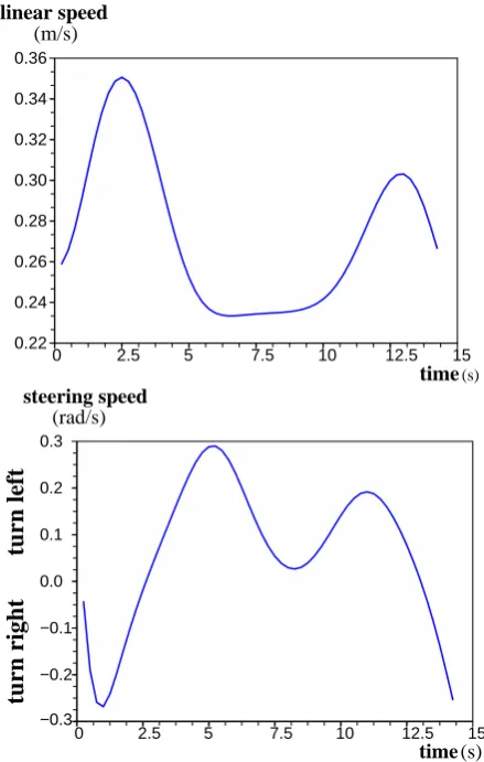
We eliminate the noise by using a low pass filter, assuming that the demonstrator didn’t do sharp changes in the heading direction while performing the desired task. We then com-puted the translational and rotational velocities of the demon-strator along the trajectory (see figure 10).

Sensorless trajectory following Having obtained the ve-locity information of the demonstrator along the desired path, we used them to drive the robot blindly in the test environ-ment. During this first robot interaction with the environment,

t=18 t=39 t=50

t=61 t=72 t=80

time(s) linear speed

(m/s)

0 0.22 0.24 0.26 0.28 0.30 0.32 0.34 0.36

2.5 5 7.5 10 12.5 15

turn left

turn right

time (s) steering speed

(rad/s)

0 −0.3 −0.2 −0.1 0.0 0.1 0.2 0.3

2.5 5 7.5 10 12.5 15

Figure 10: The translational and rotational speed graphs of the demonstrator while performing the desired behaviour shown in fig-ure 8. The noise due to the oscillatory motion of the demonstrator and also due to the lightning conditions that affect the performance of the trajectory capturing mechanism while obtaining the trajectory of the demonstrator was removed from the data by low past filtering.

laser readings and the robot’s translational and rotational ve-locities were logged in every 250ms (see figure 11).

Sensor signal encoding In order to decrease the dimen-sionality of the input space to the Narmax model, we coarse coded the laser readings into 11 sectors by averag-ing 62 readaverag-ings for each 22 degree intervals. We then used the Narmax identification procedure to estimate the robot’s translational and rotational velocities as a function of the coarse coded laser readings (u1,u2,· · ·,u11(see figure 1)).

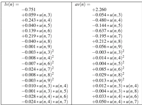
Both the translational and the steering speed model were chosen to be second degree. No regression was used in the inputs and output (i.e. l=2, Nu=0, Ny=0) resulting in

non linear Narmax structures. The both models contained 18 terms (table 2).

REX

Figure 11: The trajectory of the robot under the control of the given velocity commands obtained from the human trajectory. The robot goes along the human trajectory given in figure without using any sensory perception. During this time, it logs its own perception per-ceived along the trajectory and the velocity commands. The logged data is then used to obatin sensor based controllers which links the perception of the robot to the desired behaviour.

Model validation We then let the sensor based models drive the robot in the test environment starting from 15 dif-ferent locations. Figure 12 shows that the obtained models are successfull in driving the robot through the both door like openings without crashing into the walls.

REX

Figure 12: The trajectories of the robot under the control of sen-sor based controllers given in table 2. The robot was started from 15 different locations and it passed through the both door like openings successfully.

5.

Conclusion and Future Work

lv(n) = av(n) =

−0.751 +2.260

+0.059∗u(n,3) −0.054∗u(n,3)

+0.243∗u(n,4) −0.480∗u(n,4)

+0.040∗u(n,5) −0.144∗u(n,5)

+0.139∗u(n,6) −0.637∗u(n,6)

+0.219∗u(n,7) −0.195∗u(n,7)

−0.040∗u(n,8) +0.212∗u(n,8) −0.001∗u(n,9) −0.056∗u(n,9) −0.003∗u(n,3)2

−0.003∗u(n,3)2

−0.008∗u(n,4)2 _{+0.014∗u(n,4)}2

−0.007∗u(n,6)2 _+0.004

∗u(n,5)2

−0.024∗u(n,7)2 _{+0.085∗u(n,6)}2

+0.008∗u(n,8)2

−0.029∗u(n,8)2

−0.003∗u(n,9)2 _+0.013

∗u(n,9)2

−0.010∗u(n,3)∗u(n,4) +0.012∗u(n,3)∗u(n,4) −0.001∗u(n,3)∗u(n,5) −0.004∗u(n,3)∗u(n,8) −0.028∗u(n,4)∗u(n,6) +0.033∗u(n,4)∗u(n,6) −0.024∗u(n,4)∗u(n,7) +0.050∗u(n,4)∗u(n,7) Table 2: Experiment 3. Two sensor-based polynomials which link the perception of the robot to the desired behaviour shown in figure 11.lv(n)andav(n)are the translational velocity (inm/s) and rota-tional velocity (inrad/s) of the robot at time instantnandu1tou11 are the coarse coded laser readings starting from the right extreme of the robot

techniques.

To obtain such sensor-motor controllers, we first demon-strate the desired motion to the robot by walking in the target environment. Using this demonstration, we obtain recurrent, sensor free models that allow the robot to follow the same tra-jectory (blindly). During this motion the robot logs its own perception action pairs, which are subsequently used as train-ing data for the Narmax modeltrain-ing approach that determines the final, sensor-based models which identify the coupling be-tween sensory perception and motor responses as non linear polynomials. These models are then used to control the robot. So far we used an external, camera based motion tracking system to log the trajectory of the human demonstrator dur-ing his initial demonstration of the desired motion. Besides being expensive, such tracking systems are complicated to set up and we can not expect the end users who want to pro-gram their own robots would have this kind of facility in their houses.

Therefore we enhanced our method by replacing the Vicon motion tracking system with the Narmax polynomial models which are trained to predict the position of the demonstrator using the robot’s own vision system. The statistical analysis showed that the obtained models are able to predict the po-sition of the demonstrator with a 10±0.3cm accuracy given that the position of the jacket is computed accurately during the image pre processing stage.

5.1

Future Work

The different experimental scenarios of obtaining trajectory information using robot’s own vision system reveals that the performance of the position prediction models is dependent on how accurate the image pre processing stage extracts the

position information of the jacket from the captured images. The blob colouring algorithm is not a robust method in image segmentation especially in the environments where illumina-tion intensity is subject to noise and variant. Therefore we are currently investigating the alternatives to blob colouring algorithm which can give us more accurate positioning under different lightning conditions.

Furthermore, we are investigating the scaling properties of the presented approach, as well as methods of analysing the obtained models in order to be able to modify them off-line. Overall, the work already carried out and that proposed forms part of our ongoing research to develop a theory of robot-environment interaction.

Acknowledgments

We gratefully acknowledge that the RobotMODIC project is supported by the Engineering and Physical Sciences Research Council under grant GR/S30955/01.

References

Akanyeti, O., Kyriacou, T., Nehmzow, U., Iglesias, R., and Billings, S. (2007a). Visual task identification and char-acterisation using polynomial models.accepted for pub-lication in Int. J. Robotics and Autonomous Systems.

Akanyeti, O., Nehmzow, U., Kyriacou, T., Iglesias, R., and Billings, S. (2007b). Programming mobile robots by demonstration through system identification. submitted to European Conference on Mobile Robots.

Billings, S. and Chen, S. (1998). The determination of multivariable nonlinear models for dynamical systems. In Leonides, C., (Ed.), Neural Network Systems, Tech-niques and Applications, pages 231–278. Academic press.

Billings, S. and Voon, W. S. F. (1986). Correlation based model validity tests for non-linear models.International Journal of Control, 44:235–244.

Eykhoff, P. (1974). System Identification: parameter and state estimation. Wiley-Interscience, London.

Iglesias, R., Kyriacou, T., Nehmzow, U., and Billings, S. (2005). Robot programming through a combination of manual training and system identification. In Proc. of ECMR 05 - European Conference on Mobile Robots 2005.Springer Verlag.

Korenberg, M., Billings, S., Liu, Y. P., and McIlroy, P. J. (1988). Orthogonal parameter estimation algorithm for non-linear stochastic systems. International Journal of Control, 48:193–210.