Digital Camera Identification Using Neural Network Algorithm And Pattern Noise In Imaging Sensors

Rochester Institute of Technology

RIT Scholar Works

Theses Thesis/Dissertation Collections

5-15-2013

Digital Camera Identification Using Neural

Network Algorithm And Pattern Noise In Imaging

Sensors

Chandni Bhowmik

Follow this and additional works at:http://scholarworks.rit.edu/theses

This Thesis is brought to you for free and open access by the Thesis/Dissertation Collections at RIT Scholar Works. It has been accepted for inclusion in Theses by an authorized administrator of RIT Scholar Works. For more information, please [email protected].

Recommended Citation

R·I·T

Digital Camera Identification Using Neural Network

Algorithm And Pattern Noise In Imaging Sensors

by

Chandni Bhowmik

A Thesis Submitted in Partial Fulfillment of the Requirements for

the Degree of Master of Science in Computer Security and

Information Assurance

Department of Computing Security

Golisano College of Computing and Information Sciences

Rochester Institute of Technology

Rochester, NY

May 15, 2013

ABSTRACT

In forensic investigation of criminal cases like child pornography, image forgery, identity theft, steganography, movie piracy, insurance claims, and other cases of scientific frauds, some of the most significant challenges may be to detect the origin of an image or the photographing camera, detect forged images or hidden messages in images from retrieved digital evidence. There has been much interest in developing camera fingerprints for the forensic task of digital camera identification; that is, to be able to tie an image to it's photographing camera with high certainty or good assurance metrics, specially when the camera is not present in the crime scene. Inspired by the existing approaches of camera fingerprint forensics, this paper explores a novel approach for camera identification, based on PRNU noise fingerprint, using Artificial Neural Network (ANN) algorithm. While statistical algorithms produce probabilistic inferences based on statistical problem data, artificial neural network algorithm learns features about the problem from training data. Based on correctness of feature representations and complex mathematical processing on the training data, the neural network is able to learn or approximate any non-linear distribution very easily. As it trains on different examples, it's generalization performance on new inputs improves. In currently proposed work, first the reference fingerprint and test fingerprint are estimated based on a simple kernel based processing algorithm for PRNU coefficient estimation. Then an artificial neural network is set up in C programming language for PRNU pattern recognition based on the estimated feature values from the reference pattern data. The network is presented with training inputs and desired outputs, and based on formulated assumptions and hypothesis described in later sections, the expectation is that the ANN will be able to recognize PRNU fingerprint in images taken by the same camera whose fingerprint the ANN got trained on. A low Mean Square Error (MSE) during ANN training and testing is an indication that the ANN could report with high confidence, a match between the camera fingerprint pattern and the pattern in test image. Multilayer Perceptron (MLP) ANN with single hidden layer is proved to be a universal non-linear function approximator and can be applied to solve any complex non-linear problem. Current approach uses back propagation MLP ANN algorithm for fingerprint detection or camera identification.

TABLE OF CONTENTS

Table of Contents

SECTION I: INTRODUCTION ... 3

SECTION II: LITERATURE REVIEW ... 6

SECTION III: BACKGROUND ... 9

SECTION IV: PRNU ESTIMATION ... 17

SECTION V: PROPOSED BACK PROPAGATION ARTIFICIAL NEURAL NETWORK .... 27

SECTION VI: EXPERIMENTS AND RESULTS ... .41

SECTION VII: FUTURE WORK ... 73

SECTION VIII: CONCLUSION ... 74

SECTION IX: SKILLS REQUIRED AND TECHNOLOGIES APPLIED ... 75

SECTION X: REFERENCES ... 76

APPENDIX A: ... 81

SECTION I: INTRODUCTION

Digital representation of reality proves extremely useful when presented in cyber crime trials based on the authenticity of digital evidence. However, the simple philosophy of 'seeing is believing' cannot be trusted anymore. In digital image processing, phenomenal and rapid developments have Jed to many advanced techniques that can easily tamper with digital evidence. Image processing tools and software avai )able for free and open source on the Internet are easy prey to targeted hacks and can lead to sophisticated crimes of image tampering. In forensic investigation of criminal cases like child pornography, image forgery, identity theft, steganography, movie piracy, insurance claims, and other cases of scientific frauds, some of the most significant challenges may be to detect the origin of an image or the photographing camera, detect forged images, hidden messages in images etc. from retrieved digital evidence. There has been much interest in developing camera fingerprints for the forensic task of digital camera identification; that is, to be able to tie an image to it's photographing camera with high certainty or good assurance metrics, specially when the camera is not present in the crime scene. Inspired by the existing approaches of camera fingerprint forensics as given in [l]-[6], this paper explores a new algorithm for camera identification or device identification based on PRNU noise fingerprint. Empirically, Photo Response Non-Uniformity noise or PRNU found in camera imaging sensors has been shown to be a good candidate for camera sensor's unique identifier. This noise fingerprint is not detectable in digital images by naked human eyes, we need computer algorithms to do the processing. From empirical evidence, the task of device identification can be broken down into three sub-tasks:

l. Task A - Fingerprint generation: Camera sensor PRNU noise estimation from already known source camera images.

2. Task B: Fingerprint extraction: Once the mother fingerprint is available, extraction of PRNU noise coefficients from images under test.

3. Task C: Detection of match between the extracted fingerprint and the estimated/known camera fingerprint.

Following the basic approaches above, some previously taken images by the camera need to be present to approximate the camera fingerprint first. Then the otherwise invisible PRNU noise matrix is extracted from the test images. Previous approaches used different statistical methods like correlation detection [l], Maximum Likelihood Estimation etc. [34) to then finally draw probabilistic inferences like, what is the likelihood that extracted noise pattern from test image and the reference camera fingerprint pattern match.

The proposed thesis work explores a different approach for camera identification based on Artificial Neural Network (ANN), which is a kind of machine learning algorithm. While statistical algorithms produce probabilistic inferences based on statistical problem data, artificial neural network algorithm learns features about the problem from training data. Based on correctness of feature representations and complex mathematical processing on the training data, the neural network is able to learn or approximate any non-linear distribution very easily. As it trains on different examples, it's generalization performance on new inputs improves. In currently proposed work, first the reference fingerprint and test fingerprint are estimated based on a simple kernel based processing algorithm for PRNU coefficient estimation. Then an artificial neural network is set up for PRNU pattern recognition based on the estimated feature values from the reference pattern data. It is presented with training inputs and desired outputs, and based on formulated assumptions and hypothesis described in later sections, the expectation is that the ANN will be able to recognize PRNU fingerprint in images from the same camera, whose fingerprint the ANN got trained on. A low Mean Square Error (MSE) during ANN training and testing is an indication that the ANN could report with high confidence, a match between the camera fingerprint pattern and the pattern in test image. Although the detection technique may sound similar to statistical pattern recognition, there are fundamental differences between their algorithms, processing, approach and can outweigh each other in problem solving and performance based on fitness of implementation to the problem [36). Multilayer Perceptron (MLP) ANN with single hidden layer is proved to be a universal non-linear function approximator and can be applied to solve any complex non-linear problems [8],[12),[16),[30],[40]. Current approach uses Back Propagation MLP ANN algorithm for fingerprint detection or camera identification.

In this paper, section I introduces the problem context. Section II talks about the previously proposed statistical and neural network applications for camera fingerprint detection through a literature review. Section III gives a brief background of different image noise sources keeping in mind the forensic context, describes origin of PRNU and talks about the choice of PRNU noise as the camera sensor identifier. From section IV onwards, we delve deeper into the current work done. Based on the background laid out in the previous sections, Section IV describes current problem statement, the background of PRNU estimation and proposed hypothesis, currently proposed algorithm for PRNU estimation and extraction, and wavelet based denoising to draw a comparison with currently proposed approach. Section V gives a background of multilayer perceptron neural network and back propagation algorithm to understand their implementations in current context, the ANN based problem hypothesis, assumptions and expectations, which all go towards explaining the acquired results better. Section VI describes the scope for future work, section VII is conclusion, section VIII describes the experiments performed and results obtained for:

Tasks A and B: PRNU coefficients estimation using proposed neighborhood kernel standard deviation based filtering method. Current algorithm is inspired by adaptive block based filtering approach technique as given in [38]. An attempt is also made to compare currently proposed algorithm with adaptive wavelet filtering approach as implemented by Dr. Jessica Fridrich et al. in [1][33] for fingerprint estimation.

Task C: An artificial neural network machine learning algorithm implementation for camera identification from test images. The results are discussed. Section IX describes the skills acquired and technologies implemented, section X lists the references. Finally Appendix A contains the CIC++ code implementation.

SECTION II: LITERATURE REVIEW

To better understand the significance of the current approach, this section overviews some of the previous research most relevant to our field of investigation. Dr. Blythe, P. and Dr. Fridrich, J (August 11-13, 2004) in the paper "Secure Digital Camera" presented at the Digital Forensic Research Workshop, reported one of the simplest ways to figure out image origin by looking at the image file meta data'

[9]. For example, the EXTF image file specification or a Jpeg image file header reveals a lot of useful information like image time stamp, camera settings, image thumbnail, description and copy right information etc.

Advantage: This is one of the simplest and most inexpensive methods for image origin check. Problem: The meta data available with the electronic image file can be easily tampered with or modified. This method does not guarantee image file integrity, thus the meta-data cannot be trusted as evidence in court [l].

Another approach in practice by Canon, the Canon Verification Kit [IO], secures cameras with embedded digital watermark. Digital watermarking is defined as the process of embedding information into a digital signal to be used later for verifying authenticity of the signal or identifying its owner [28]. This digital watermark by Canon embeds camera information, image time stamp, user bio-metric data etc directly and securely in each image.

Advantage - Every image produced by such a 'secure' camera contains its integrity and origin information embedded in itself. Problem - Not all cameras are secured in this fashion. Using camera watermarking technique can be expensive and therefore not used in cheaper commercial cameras.

Support Vector machine learning algorithm or SVM, an artificial intelligence technique, is implemented by Kharrazi et al. in [ 1 I] for feature based classification of digital images. In this experiment, SVM was used to model and train an artificial learning agent to classify a set of images under 5 different cameras, based on certain

Image meta data helps to determine certain features of the image like make and model of the camera used to capture the image, image time stamp, exposure settings of the camera etc [27];

features. The classification outcome produced 78% worst case and 95% best case accuracy.

Advantage - SVM, as a machine learning concept, is known for its huge commercial success. It allows computers to deal with large number of features for feature based classification problems [ 12]. Problem - For presenting as trust worthy evidence in court, higher outcome accuracy is desirable.

Kenji Kurosawa et al. in [13] proposed identifying defective pixels in images as dark or bright dots and establishing the camera fingerprint merely based on such defective pixel distribution. In imaging sensors, defective pixels can be defined as pixels that fail to sense light levels correctly [29]. Therefore, a defective pixel can either sense no I ight at al 1 leading to a dark spot appearance or can be totally saturated and appear always as a bright spot. In either case, such defective pixels fail to register the proper incident light intensity.

Advantage - The advantage lies in the relative simplicity in analyzing hot or dead pixels. Problem - In most of the modern digital cameras in use today, defective pixels don't survive image post-processing. Therefore this approach would fail in the absence of any data [ 1].

Other approaches for camera identification involved use of photo-response non uniformity or PRNU noise in images. Pattern noise in a digital image is described as any noise that survives frame averaging [14]. PRNU and dark current are two such pattern noise that accumulate in images during image acquisition cycle [3]-[4]. Previous work by Dr. Jessica Fridrich et al. in [1]-[2], [5]-[6] and Kenji Kurosawa et al. in [ 15] proposed PRNU and dark pattern noise respectively for camera fingerprinting. Both the approaches produced significant improvements over defective pixel analysis that didn't survive image post processing in modern cameras.

Authors in [1]-[4] and [6] implemented statistical correlation, a computationally heavy brute force fingerprint detection mechanism that does not work well when geometrical operations such as cropping, rotation, zooming etc. are involved in images. This technique for camera identification is based on examining the correlation between the camera fingerprint and extracted noise in test images. By building a database of test images by different cameras and calculating statistical

correlation for fingerprint detection for each of the test images, the result confirmed that, the correlation between the fingerprint and the noise residue is highest in images by the camera whose fingerprint is being detected. This processing and correlation detection have to be on continuous image kernels; it would not work on disjoint pixels. Also for large images with a lot of pixels, this mechanism can significantly degrade in performance [ 1].

Authors in [ 15] detected dark current noise as the unique camera fingerprint 1n an image. But the method is restricted to only dark frames.

ANN machine learning approach is different conceptually and operationally. It does not suffer from some of the common short comings of the previous approaches, as discussed in more details in section III.

SECTION III: BACKGROUND

CCD CAMERA IMAGING AND SENSOR NOISE

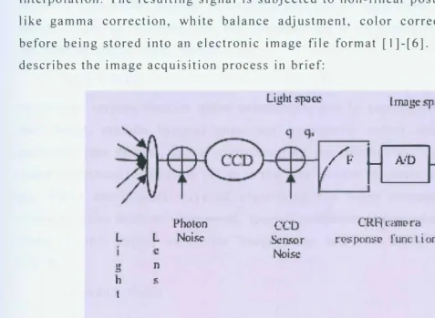
Different noise sources accumulate in images during the image acquisition life cycle. Modern high-end cameras do post processing to improve image quality by suppressing such noise. In an ideal digital camera, light reflected by the object under capture hits individual pixels in an imaging sensor array, a CCD or CMOS, covered with a color filter array (CFA) so that each pixel registers exactly one color out of Red, Green and Blue (RGB). The total color value for each pixel is later obtained through color interpolation. The resulting signal is subjected to non-linear post processing functions like gamma correction, white balance adjustment, color correction, sharpening etc before being stored into an electronic image file format [I]-[6]. The following figure describes the image acquisition process in brief:

L L

g n

h :S t

Li �ht space

P'hoton

CCD

Noise- _Scnc;or

Noise-/F

I mn

�c-sp.i1Cc-��

,Lr

CR!i cane rn

response func l ion)

Figure 1: CCD Imaging System2

Chao Deng and Bi Bo Lu, "Applying an Improved Neural Network to CCD Noise Removal in Digital Images," in 2009 Second Int. Conference on Inform. and Comput. Sci., 2009 © IEEE, pp. 136, Fig. I, doi: I0.1109/ICIC.2009.143;

[image:12.766.35.513.334.683.2]

CCD NOISE ANALYSIS

From a forensic perspective, to better understand the significance of using PRNU noise as the camera fingerprint, it is deemed important to understand the background of different image noises. This section provides a brief overview of different noise sources that accumulate in a digital image. Based on current discussion, an attempt is also made to describe device identification problem modeling in the light of artificial neural network algorithm.

Ideally, as light hits the imaging sensor, the amount of electrons or charge produced at every pixel of the resultant image should be exactly proportional to the intensity of incident light or the number of incident photons on each pixel. If IN [i] denotes the sensor output or response and Ic [i] denotes the clean signal input at each pixel i of the camera sensor, then ideally,

IN [i] oo Ic [i] ... (1)

In reality, various random noise components due to sensor inefficiency, photon and shot noise, random thermal noise and systematic noises due to vignetting, dust particles, Jens defects, sensor manufacturing inconsistencies, sensor dark current etc. cause variations to equation (I) or to the ideal sensor response IN [i] with respect to le [i]. There are several ways of classifying the noise components based on their characteristics such as - temporal, spatial, temperature dependent, random or pattern noise. In this paper, we divide image noise into two broad categories as follows [l]-[6]:

- Random Noise.

- Pattern Noise.

Random noise - This consists of Dark Current Shot noise and Photon Shot noise.

Photon noise arises due to the difference in the number of incident photons on two equally sized pixel areas on an imaging sensor exposed to the same light intensity. The difference in photon counts varies randomly between pixels, hence the random nature of the noise as described in [17] and [18].

Photo electrons also contribute to Shot noise. The number of electrons at any particular point in the path of an electric current fluctuates randomly giving rise to shot noise as described in [3], [4], [19], [20] and [21]. Random noise under totally dark conditions is called dark shot noise which also includes other signal independent on-chip amplified random noise sources [3].

Pattern noise - This consists of the deterministic component of image noise. This kind of noise is relatively stable in images taken by the same camera (or same CCD sensor) but varies for different CCD chips.

Pattern noise can be further classified into:

Fixed Pattern noise (FPN) or Dark Current noise - Dark noise is introduced by small amount of electric current flowing through a photo sensitive device like CCD in the absence of any incident photons. The number of electrons generated in a second depends on the camera exposure and also the operating temperature of the CCD.

Therefore it is also known as the thermal noise as described in [3]-[4], [19] -[ 22].

Photo response non-uniformity (PRNU) - PRNU pattern noise arises due to non-uniform photo-active areas during manufacturing process of the imaging sensor hardware, CCD3 _{or CMOS}4_{, and due to material properties of silicon. [33] [39]. This} induced noise affects the way pixels on the camera sensor respond to light intensity [l]-[6], is quite stable across images taken by the same camera but varies for different CCD chips. Due to it's properties, PRNU noise is treated as a unique candidate for camera sensor fingerprint. PRNU is mainly dominant in higher signal intensities; part of this noise is also due to low-frequency spatial defects from dust particles on the lens, shape of the aperture, zoom settings and vignetting and contribute to 'dough-nut' pattern noise in the image [l]-[6], [19]-[22].

These different noise sources couple up with the actual signal le [i] to produce a noisy output pixel. Camera fingerprint estimation by current approach requires only

CCD or Charge Coupled Device is a major technology for digital imaging. CCD imaging sensor is a device used mainly for movement of electrical charge. Capacitor bins on the CCD allow incoming photons to transform into electric charge which is then shifted or moved within the device one electron at a time to an area where the charge can be manipulated, for example conversion into a digital value[26];

4 Complementary metal-oxide-semiconductor (CMOS);

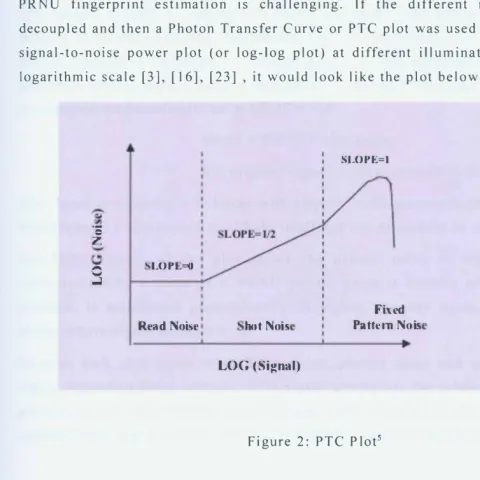
the PRNU coefficients to be separated out from an image's final noisy output. Given the complex factors associated with image denoising due to some of the complex inter-dependencies between different noise sources and image signal, the task of PRNU fingerprint estimation is challenging. If the different noise sources were decoupled and then a Photon Transfer Curve or PTC plot was used to show the average signal-to-noise power plot (or log-log plot) at different illumination intensities on a

logarithmic scale [3], [16], [23] , it would look like the plot below in an ideal case .

• iLOPv=l

=

z

:,

..;i

"LOP1£=11

Read Noise hot Noh

LOG (Signal)

Fiud P'attern Noi,;

Figure 2: PTC Plot5

The above plot can be interpreted as:

X axis - shows the clean image signal strength;

Y axis - shows the noise coefficients strength;

5 Gardner, D. (n.d.). in "Characterizing Digital Cameras with the Photon Transfer Curve". Retrieved from Summit Imaging website: http://www.couriertronics.com/docs/notes/cameras application notes/ Photon Transfer Curve Charactrization Method.pdf, pp. 2, Fig. 2;

[image:15.761.34.515.164.645.2]

The first domain of the plot is characterized by read out random noise where signal to noise ratio is a flat curve. This signifies that read-out random noise is independent of the imaging signal and present in low intensity pixel areas.

The second domain of the plot is characterized by shot noise. Shot noise can be defined as an impulse noise that randomly alters some pixels. Since the time between photon arrivals is governed by Poisson statistics, the uncertainty in the number of photons collected during a given interval also follows Poisson distribution and can be represented mathematically as: u SHOT= ...JS;

where cr SHOT = shot noise;

S = _{original signal, both expressed in electrons [3].}

The signal to noise ratio is linear with slope = _{Y2. Shot noise is therefore more signal} dependent, is a characteristic of light itself and not dependent on camera sensor.

The third domain of the plot shows the pattern noise to signal ratio which is characterized by a slope of I. PRNU pattern noise is directly proportional to signal strength, is manifested predominantly in higher intensity areas, and is seen to be absent where signal strength I- 0.

Random dark shot noise or read-out noise, photon noise and pattern noise are all signal dependent noise sources. With signal averaging, the random noise components get suppressed while pattern noise becomes more dominant in the image. In expensive cameras with larger imaging sensors, shot noise is greatly minimized.

MATHEMATICAL MODELING OF SENSOR NOISE

Based on the previous discussion, the ideal sensor output signal from ( 1) is subjected

to additive6 _{random noise, dark current noise and multiplicative}7 _{PRNU noise. Finally}

the signal goes through complex non-linear digital signal processing before being

saved into electronic files. For camera identification, PRNU is our noise of choice. As described in [ l ]-[ 8], to extract on I y the PRNU coefficients out of the noisy fin al sensor output, a ma them a ti ca I mode! of the sensor output sign al IN [ i] at each pix e I i, affected by noise sources, can be given as follows [l]: As compared to equation (1), in reality, the sensor output can be modeled as:

IN= le + Ie*K + D + 8 ... (2)

where IN€ R/\_{(m x n)} = _{Matrix of noisy output signal per pixel i of a 2-D image} sensor;

le€ R/\_{(m x n) = Matrix of clean signal or DC at each pixel i of a 2-D image}

sensor; This is the true incident light intensity transformed through a linear photon to electron transfer curve without any additional sensor response added or multiplied.

K € !Rl,"(m x n) = Matrix of PRNU coefficients at each pixel i of the 2-D image sensor;

D = Dark Current;

e = Other random noise sources.

Additive Noise: If random noise coefficient is added to the true pixel intensity to generate noisy output, the noise is additive [31].

Multiplicative noise: If random noise coefficient is multiplied to the true pixel intensity to generate noisy output, the noise is multiplicative [31 ] ..

We can describe the manifestation of PRNU noise in image scene as, the true image scene matrix le being laid over by noise matrix K modulated by signal le (noise matrix k = element wise product of matrices true image scene le and PRNU coefficient K) (33]. Following statistical concept, at a particular exposure and temperature, PRNU coefficient value at each pixel can be modeled as an independent, identically

distributed (i.i.d)9 _{Gaussian random noise variable}10 _{that multiplies to the true incident}

intensity value of that pixel. The Gaussian probability density function11 _{of PRNU}

coefficients per pixel is characterized by a local standard deviation cr[i,j] and local

mean µ[i,j] = 0 at pixel position (i,j) of a 2-D image. To observe PRNU characteristic

K [ i ,j ] from ( I ) an d ( 2) , we need to de r i v e ( 3 ) as fo II ow s :

IN =le +le *K ... (3)

In (3), K € JR"<m x n), that is, K can take any random value on the Real Number line between negative and positive infinity. However, PRNU values in digital cameras are generally restricted between -1 and +I (33].

Also the noise strength K cannot be detected where le � 0 or if le > sensor pixel saturation. Therefore, PRNU cannot be observed in too dark or saturated sensor pixels. Pixels with highly non-uniform photo response may give rise to very bright or very dark points compared to the rest of the image.

i.i.d noise: Independent Identically distributed noise. Independent means, the joint probability density function of all the random noise coefficients in the image can be expressed as the product of individual probability density functions. Identically distributed means, all the noise coefficients follow identical probability density functions [31 ).

10 Gaussian noise: Random noise value at each pixel position (ij) that affects the true pixel value is drawn from a Gaussian probability density function with meanµ (ij) and standard deviation cr (ij) [31).

11 _{Probability density function: If data vector y} = (y, .... Yn) _{is a random sample drawn from an unknown population of samples,} where a population is defined by a unique probability distribution characterized by unique parameter w, the probability density function is a statistical computation to determine the most probable population that generated the sample, given data vector Y and parameter W [34).

SECTION IV: PRNU ESTIMATION

CURRENTLY PROPOSED APPROACH

For PRNU computation, the image noise acquisition physical phenomenon is exposed as the sensor output mathematical model as previously mentioned in equation (2).

From equation (2),

IN= le + Ie*K + D + e

where IN€ Il�:"(m' nJ = Observed noisy output signal.

le € R"(m' nJ = Clean signal or DC at each pixel i of a 2-D image sensor; This is the true incident light intensity through a linear photon to electron transfer curve without any additional sensor response added or multiplied.

K 8 �A_{(m x n)} = Matrix of PRNU coefficients at each pixel i of the 2-D image sensor;

D = Dark Current;

8 = Other random noise sources.

Current Assumptions for devising PRNU Estimation Algorithm are

• Working with RAW format images: The Nikon DSO camera used for this

experiment was programmed to output RAW format images (.NEF) without any kind of scaling on the raw intensities registered at each output pixel of the CCD sensor. The assumption is that, since cameras generally apply non-linear post processing like white balancing, gamma correction etc. on the raw sensor output before finally storing the image data in electronic format in memory, this added non-linearity may further obstruct our PRNU estimation. Therefore, we will work with raw sensor output images in proposed approach.

• Opted out of color channel interpolation: As previously described in section Ill, due to the CFA in front of the camera sensor, each pixel of the sensor registers only one color out of Red, Green and Blue or RGB if the camera color profile is RGB based. This is implemented with a Bayer pattern filter that looks like this:

Figure 3: Bayer filter pattern [3612 ]

In our case, Nikon D50 uses RGB color space for imaging. To obtain the final pixel output for a true color image from a gray scale Bayer pattern filtered image, the camera applies a non-linear interpolation so that every pixel has RGB data to produce the true scene color. Since this interpolation will also add to the signal non-linearity, once we have our raw frames (non-interpolated), an algorithm is devised to figure out a way to identify and separate the R, G and B channels from the gray-scale non-interpolated raw images and save them into separate color channel frames [Appendix A]. The concept is shown in the figure below. Once that is achieved, we only work with the green channel frame since it has the maximum data.

12 From Wikipedia article on Bayer filter website Bayer filter.(2013, April 23). Retrieved April 30, 2013, from Wikipedia website: http:! /en. wikipedia.org/wiki/Bayer _filter

[image:21.764.17.505.66.358.2]

Incoming light

Filter layer

Sensor array

II

II

• Result;ng pattern

Figure 4: Separate RGB channels [3613_]

• Working with white images: As stated in the noise characterization section, PRNU is modulated by the clean image signal. Therefore, for PRNU calculation from previously taken images by the target fingerprint camera, it is desirable for sample images to have flat illumination gradient, like image of a white board (if clicked indoors) or blue sky (outdoor photography). Since properly lit images without scene are flatly illuminated, true PRNU values are easier to estimate without much modulation by fluctuating signal intensities from real scenery.

• Dark noise removal: Dark current D, which also qualifies as pattern noise, 1s most prominent in dark frames. Dark noise can be removed by subtracting a master dark frame from the white image averaged signal to nullify dark current pattern noise contribution to PRNU.

• Frame averaging: Random noise components like photon or shot noise can be easily suppressed by frame averaging. Therefore, for PRNU coefficients estimation per pixel, we work on final signal averaged over multiple white images by the same camera.

• Based on equation (2), after dark current removal and random noise suppression from observed noisy signal IN, we are left with:

13 From Wikipedia article on Bayer filter website Bayer filter.(2013, April 23). Retrieved April 30, 2013, from Wikipedia website: http:! /en. wikipedia.org/wiki/Bayer _filter

[image:22.756.58.520.73.612.2]

h - D - 8 = (le + Ie*K + D + 8) - D - 8

le + Ie*K

IN' = le + Ie*K ... (3)

This resultant signal IN' has PRNU factor K as the dominant noise pattern. • Photo-response coefficient esti ma ti on: In equation (3 ), the derived s igna I

IN' = (clean signal le)+ (signal non-uniformity lc*K).

The assumption is that, if we can estimate the clean signal le as le' and divide IN' by estimated le', we will obtain the PRNU factor K as:

IN' = _{le+ lc*K}

(IN'

I

le')

=

(le + le*K)/le' ... ( 4)

Further, based on the accuracy of DC estimation, the assumption is, estimated le' and true le will cancel out.

(IN'/ le')= (I + K) when le == _{le' ... (5)}

CLEAN SIGNAL OR DC ESTIMATION - CURRENT APPROACH

The proposed algorithm is applied to PRNU coefficient estimation from a plain, flatly illuminated white image as well as a real image with content. Images used in the experiment are from the Nikon D50 camera. An adaptive, kernel based standard deviation algorithm, as devised in current approach, is described below:

o After averaging multiple white image frames to suppress random noise and then subtracting a master dark frame from the averaged white frame, we get the reference frame based on which PRNU coefficients for the camera sensor will be estimated. At this stage, we are at equation (3).

0 Next, the averaged frame containing the signal IN' from (3) is segmented into N square kernels, each of size n by n, for processing.

o Assumption is that, instead of considering the whole image for clean signal estimation, we only look at the 'smooth' kernels; 'smooth kernels' are those with relatively low signal variance or standard deviation compared to the rest of image. This facilitates PRNU estimation and detection since a hot pixel in the center of a smooth kernel neighborhood will indicate a non-uniform pixel response compared to surrounding smooth pixels. Once we find all such kernels that qualify as smooth, we average only the smooth kernel pixels to find averaged clean signal or estimated DC.

0 Once we have the estimated DC, we divide observed IN' by estimated DC or le' following equation (4) to arrive at equation (5) as given above.

o Algorithm for finding relatively smooth kernels is as follows:

1. Go through each pixel in the image.

2. For current pixel, construct an k x k kernel neighborhood considering the current pixel as the kernel center.

3. Find standard deviation of current kernel. Do not include the central kernel pixel data in the standard deviation calculation. For computation, the assumption is that the center is the hot pixel as compared to the smooth surrounding.

4. Repeat 2 and 3 for every pixel and kernel neighborhood around that pixel across the whole image, including corner pixels. This will give an array of kernel standard deviations. Note: Since the corner pixels of an image will not yield a full k x k kernel neighborhood, we work on partial kernel data. This is appropriate for DC estimation since we don't want to skip any observed signal data.

5. From 4, find the minimum standard deviation, this is our smoothest kernel.

6. Go through each pixel neighborhood kernel standard deviation value as calculated from step 4.

7. If (current kernel standard deviation)<= (minimum standard deviation + 1/10 * (maximum standard deviation - minimum standard deviation)), consider the current kernel pixels for estimating DC signal. By

calculating (minimum standard deviation + 1/10 * (maximum standard deviation - minimum standard deviation)), we create a very simple low pass filter that penalizes the upper 90% of the signal intensities while selecting only lowest 10% as the smooth kernel intensities. Here

(minimum standard deviation + I /10 * (standard deviation range)) is the filter upper threshold.

8. Once we have compiled all such smooth kernel pixels, we average the pixels, this time including the hot central kernel pixel to arrive at our estimated DC.

o To give a brief example of how the kernel based calculation will find the smoothest block, here is an example:

*******3 X 3 KERNEL NEIGHBORHOODS************

1 2 I 11 1 9 I 11 1 2 1 11 I 2 I 11 9 2 9 11 I 9 I 11 2 9 I 11 9 9 9 11 1 1 I 11 I 9 I 11 1 2 1 II 1 9 2 II 2 I 2 II I 2 I II 9 1 9 II *Kl *ll*K2* ll*K3* ll*K4*ll*K5*

The above example shows 5 hypothe tical 3 by 3 kernels - K 1, K2, K3, K4 and K5 with pixel data, such that, kernels K 1, K2, K3 and K5 have hot pixels in the kernel center while kernel K4 is truly a smooth kernel. Following shows the basic comp utation in the c urrently proposed DC estimation algorithm above. Since K4 is the only smooth kernel here, the comp utation resul ts in selecting kernel K4 for pixel averaging to

estimate DC. This is how the proposed clean signal estimation program would work.

* DC SIGNAL KERNELS ARE KERNELS WHERE:

Kernel Standard Deviation <= (Minim um Standard Deviation +

-

-

-

-1 /-1 O(Standard Deviation range across the whole image)

* COMPUTE:

* Kl Std Without Center_{- -} = _2.61397. * K2 Std Without Center_- = 3.85501.

-* K3 Std Without Center_{- - -} = 3.77492.

* K4 Std Without Center_- = _0.44096.

-

-* MIN STANDARD DEV:-

-K4 Std Without Center_{- - -} = _0.44096.

*MAX STANDARD DEV:_-

-K2 Std Without Center_{- -} = _3.85501.

-*(MAX_STANDARD _DEV - MIN_STANDARD _DEV) /10 0.341405.

RANGE

*MIN STANDARD DEV + RANGE = 0.44096+0.341405 = _{0. 7 82365.}

*ONLY ***** K4 Std Without Center***** = 0.44096 _{- - -} < 0.782365. K4 is indeed the smoothest kernel here. This example shows that

currently proposed algorithm is able to find the smoothest signal for DC estimation. Including the central kernel pixel while DC averaging allows adaptive filtering of signal (IN') when divided by estimated DC le'. That is, higher intensity kernels will have a higher DC versus lower intensity kernels. Subtracting 1 from (5) leaves us with,

K' = (IN' I le') - I = ( 1 + K) - 1 = K ... (7)

Here, K' is the estimated photo response. From (6), when K' = K = 1, it is uniform photon to electron transfer response. Based on K < 0 or K >O, the otherwise uniform sensor response will be amplified or suppressed due to PRNU factor K.

WAVELET FILTERING PRNU COEFFICIENT ESTIMATION

1. At higher intensities, the PRNU random noise coefficients are overshadowed by additive shot noise which is modeled as a white Gaussian noise distribution in this approach.

2. The sensor output mathematical model given in equation (2) can also be represented as in [33): IN= K *(le + shot-noise) + D + 9 ... (8)

This approach attempts to improve the signal of interest to noise ratio by wavelet based filtering of this non-stationary Gaussian white shot-noise.

3. From (8), after suppressing random noise components by averaging white frames and subtracting dark current from the master white signal matrix IN, we

arrive at:

IN= (K*(lc +shot-noise)+ D +

e) -

D -

e.

K * (le + shot-noise)

le* K + K *shot-noise ... (8.1)

4. Then wavelet filtering as described in [1] is applied to filter out white Gaussian noise coefficients from (8.1). The filtering results in IN' with signal and PRNU but denoised of white Gaussian noise.

IN'= F(IN ). IN'= K * (le)+ (c) ... (8.2)

where c is non-linear response introduced by the wavelet denoising filter

Here PRNU defective component Ic*K is the signal of interest.

5. Since this white Gaussian noise is not independent of PRNU, the denoising affects PRNU strength reduction. Currently proposed approach does not rely on white Gaussian noise filtering in this way. It is assumed that averaging multiple frames suppresses random noise components like white Gaussian shot noise.

6. This denoising also introduces an additional non-linear random component to our mathematical model in (2). Current approach introduces no such additional component to the observed data.

7. Finally, to obtain K from 8.2, it is assumed that K is very weak compared to le and therefore le assumed to be independent of K.

Therefore dividing by le on both sides of equation (2.4) yields,

IN'/ le.= K +(€)/le .. (8.3)

SECTION V: PROPOSED BACK PROPAGATION ARTIFICIAL

NEURAL NETWORK

Before describing currently proposed neural network algorithm and results from current experiments, in this section I will introduce briefly the historical background of machine learning algorithms and their value addition to traditional programming. This may be beneficial to understanding the inspiration behind proposed neural network approach for camera identification.

Artificial Neural Network (ANN) Machine Learning (ML) algorithms are favored for tasks like object recognition, pattern recognition, speech recognition, prediction etc. Problems like these are fairly easy for a human brain to solve while computer programs need very complex algorithms. The complexity stems from the fact that computer programs need every step of the problem and solution to be hand coded for writing good programs and we need to decode how the brain exactly works out the problem. The human brain is immensely complicated and much research is going on in neuro-science in determining how it exactly works. ANN is a novel learning algorithm inspired by the brain and implemented by parallel distributed computing.

To give a simple understanding of how artificial neural network machine learning algorithm is different in approach from previously proposed methods for camera detection, I refer to the following two definitions of machine learning (ML): Field of study that gives computers the ability to learn without being explicitly programmed (Arthur Samuel, defined 1959) [8].

A computer program is said to learn from experience E with respect to some task T and some performance measure P, if its performance on T, as measured by P, improves with experience E (Tom Mitchel I, defined 1998) [8].

To extend the given definitions of machine learning to our problem context, defined below are some basic ML terminologies as mentioned in [8], [ 12]:

- Task being learned. In this case, the task is PRNU pattern recognition by approximating a hypothesis function that best fits signal to PRNU noise behavior.

- The training or experience E. This can be supervised, unsupervised or reinforcement training as explained in [8], [ 12]. Proposed algorithm in current thesis applies supervised training on images.

- Goal of training. This indicates some prediction, diagnostic or summarization that the problem cares about [8] [12]. This is the desired outcome. In this case, the desired outcome is correct prediction of photo response non-uniformity coefficients per pixel of a 2-D camera sensor.

- Output of machine learning hypothesis. While in a regression problem, the outputs of a neural network learning algorithm are continuous values, in case of a classification problem, it is generally a binary output unit that gives a linear decision boundary that divides the solution space into two classes. In current thesis, the output of the neural network algorithm is a continuous value € R, depicting the PRNU coefficient of each sensor pixel.

Stitching the terminologies together, a machine learning algorithm uses the experience gained from training examples to learn the functional mapping between some feature vector X and the target label Y such that in future it'll be able to predict Y based on new but similar category of features X. Work done in [8], [12] are good sources to gain more background in machine learning in general.

THESIS: DIGITAL CAMERA IDENTIFICATION USING NEURAL NETWORK ALGORITHM AND PATl ERN NOISE IN IMAGING

BIOLOGICAL NEURON

In biological terms, a neuron is a functional unit in the brain that communicates with other neurons by means of electrical signals or sparks [36].

• Each neuron receives inputs from other neurons.

• The effect of each input is governed by the synaptic weight.

• An electrical spark gets generated at the synapse and injected to other neighboring neurons through the dendritic trees.

• The weights adjust themselves to learn problems and produce required outcomes.

• A collection of multiple neurons forms a functional neural network that enables the brain to work the way it does. In human brain, there are about 10/\ ₁₁ neurons each with about l 0/\ _{14 weights.}

Figure 5: Structure of biological neuron 14

14 _{Axon hillock. (n.d.). Retrieved May I, 2013, from Wikipedia website: https://www.google.com/search?}

q=axon+hillock&safe=_off&tbm=_isch&tbo=_u&source=_univ&sa=_{X&ei=sTe8Udr6KKbEigLAwlHAAQ&ved}=_OCDsQsAQ &biw=_l536&bih=_776#imgrc=_{WgF-2HmU57C7_M%3A%38Xe3E07hTrlmM5M%38http%253A%252F}

%252Fwww.seattlerobotics.o rg%252Fencoder°/o252F200205%252Fprj3%252Fabionin _fig I .jpg%3 8http%253 A %252F %25 2 Fwww .seattlerobotics.org% 2 52 F encoder%2 52 F20020 5%2 52 F ab ion i n.htm%3 83 8 7%3 8220

ARTIFICIAL NEURAL NETWORK (ANN)

An artificial neural network (ANN) is a machine learning algorithm that tries to mimic the brain [30]. Each neuron is implemented as a processing unit or node and a collection of such functional nodes forms an artificial neural network that is capable of modeling any given problem, based on the amount of information that the network can store or process, depending on the related network complexity. Data heavy or feature rich problems may make neural networks computationally expensive, however modern computer technology today is gaining faster processing speed to cope with this state of the art technology [ 16], [7] and [8].

PERCEPTRON

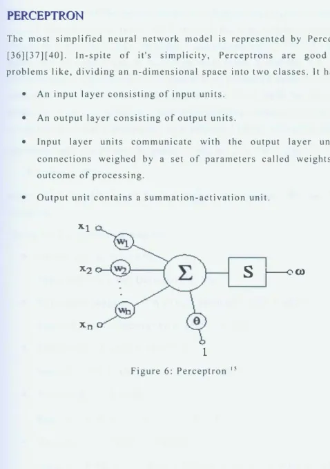
The most simplified neural network model is represented by Perceptron [7][12][30] [36][37][40]. In-spite of it's simplicity, Perceptrons are good at classification problems like, dividing an n-dimensional space into two classes. It has:

• An input layer consisting of input units.

• An output layer consisting of output units.

• Input layer units communicate with the output layer units by means of connections weighed by a set of parameters cal led weights that control the outcome of processing.

• Output unit contains a summation-activation unit.

x1

X2

s

L...,__/'\

m

Xn

1 Figure 6: Perceptron 15

15_{Figure from Dawson, M. R. (2004, November 17). Rosenblatt. Retrieved May I, 2013, from}

Biological computation project artificial neural network software website: http://www. bcp. psych. ual berta .ca/-m i ke/ Software/Rosen b I att/

[image:34.761.43.522.74.754.2]

The above figure of Perceptron shows an n-dimensional training data vector X={x1, x2 .

... xn} from the input layer travel through the connections, parametrized by weight vector W = {w1, W2, .... wn}, to reach summation unit L· The

I

unit is placed right before the activation unit S. Based on total input X and the hypothesis function or activation he(x ), parametrized by vector 8, an estimated value for the target label w is generated. The summation unit generates the total input by summation of the dot product of each incoming input and corresponding connection weight. The dot product is compared against a activation value generated by the activation function he(x ).

Mathematically, total input X, parametrized by vector 0 is given by [8]:

X= (0oxo +0 1x1);

where Xo is input bias and X1 is a single input feature. 80 and 81 are connection parameters.

The activation function S may be: • Linear, y = ho (x) = x*s.

Span: -inf< y <inf.Derivative d: I *s.

• Hyperbolic tangent, y = h 0 (x) = tanh(x) = 2/( 1 + expc-2•s•x>) - 1.

Span: -1 < y < 1. Derivative d: s*(l - (y*y)). • _{Logistic, y = h e (x) = ( 1 +e-s*x)-1.}

Span: 0 < y < 1. Derivative d: s*y*( 1-y).

• Threshold, y

=

he (x).

Span: x < 0 -> y = 0, x >= 0 -> y = 1. • _{Gaussian, y = h 0 (x)} = _e(-x2/2).

Span: y = 0 when x = -inf, y = l when x = 0, y = 0 when x = _inf. Derivative d: -2*x*s*y*s.

MULTIL AYERPERCEPTRON(MLP)FEE DF ORWARDNET WORK

In MLP network, the input units do not directly communicate with the output units. Instead, there is at least one hidden layer of nodes in between the input and output layers. Given inputs to the input nodes, it forward passes the signal to the hidden or inner nodes of the network which do the main processing. Upon feeding the initial input values to the network's input layer, each input gets multiplied by the weights of the connections it traverses. At each receiving node in the hidden layer, a summation unit sitting right before the node's activation unit, accumulates all (inputs*weights) values coming into that node via weighted connections. The output of each hidden node. based on the input strength (inputs*weights), is then accumulated in a similar fashion and propagated to each output layer node. The activation output of a node is high only if the input vector lies within the node's decision boundary. The hidden layer function can be seen as logical AND operation, each producing independent predictions based on the total input and individual node's decision boundary. While the output layer can be seen as a logical OR operation where the goal is, to depict the most probable outcome for current input out of all the possible outcomes. After the input signal traverses through all the nodes of the hidden and the output layer, the final output of the network is compared with a desired outcome and if they are not the same, an error is calculated. This series of transformations from the inputs to the output is called Feed forward neural network training.

Error E: 1/2 * I(h0(xi) - Yi)2· where he(xi) = output from ANN node j.

Yi= Desired output from node j.

As the output changes in favor of or against the final desired outcome, the output error rate changes. Since output of a node is the activation response due to (inputs*weights), the connection weights going into the node are adjusted accordingly such that the mean square error between desired and calculated outcome is minimized over a set of training data. However, desired outcomes are specified only for the output layer. Therefore, instead of considering the hidden layer activities as desired state, the error derivative with respect to hidden layer activity is considered for perturbing incoming weights to hidden layer nodes, a novel approach in MLP called

Back-propagation algorithm. This allows all the network wights, including the output and hidden layers to be adjusted.

MLP LEARNING RULE & WEIGHT ADJUSTMENT THROUGH

BACK

-

PROPAGATION

• MLP requires the activation function to be differentiable to calculate the error derivative.

• Logistic, Gaussian, Hyperbolic tangent are all examples of differentiable activation functions.

In currently proposed algorithm, the hidden layer activation function 1s designed to be Gaussian symmetric while the output activation function 1s Hyperbolic Tangent (tanh) to limit the output between -1 and 1.

Hyperbolic Tangent activation function:

h o (z) = tanh(z) = 2/( I + exp<_·2•2>) · 1 where

z = b + Li (x;*w;) is the total input to an activation unit and b = bias ... (9)

• In back-propagation, the weight adjustment follows the chain rule to get the derivatives needed for learning all the weights of the network. The chain rule is given as follows:

� Find derivative of output with respect to activation which is calculated as: dy/dz = (1 - y2_{) •••••••••••••••••••••••••••••••••••••••••••••••••••• (10)}

� Find derivative of activation with respect to incoming inputs and weights as: 0 z/ 0 w;= _{X; and O z/ 0 X;} = _{W; ... ( 11)}

o Find derivative of output with respect to weights in order to perturb the weights for better network performance. This is calculated as: 8 y/ a w; = (8 zl

a

w i) (

a

y /

a

z)

• From (I 0) and ( 11 ), we have,

a

y/

a

W; = X; (1 - y2) •.•..•. ( 12 )

• Finally for perturbing incoming connection weights to hidden units, find the derivative of error with respect to weights as:

a

El

a

W; = Ln (8 y"/ 8 W;)( 8 E/ 8 y") ... (14) where n total

number of output units.

• From (13), a yl a wi = xi (I - y2). Therefore, fitting value of 8 yl a wi into

(14), we get, 8 El 8 wi = Ln ( X;" (1 - y2") (hn - Yn ) ) ... (15)

• Here x;" * (hn - Yn ) is called the delta rule which is used for changing weights

in linear neurons. And (1 - y2_{") is the slope of hyperbolic tangent function.} Equation (15) is the MLP learning rule.

BACK PROPAGATION

Based on the above derivatives a back propagation algorithm works like: [45]

I. Instead of using activities of hidden units as desired outcomes, the error derivative with respect to hidden layer activities are observed. The hidden layer, as the name suggests, consist of the inner working of the ANN based on complex mathematical computations and is often considered a black-box in terms of the visibility of operations.

2. Since a single node in hidden layer affects all the nodes in the output layer, if there are multiple output nodes, the error derivatives of individual output node with respect to the hidden layer activities need to be accumulated.

3. Following the learning rule above in equation (15), once the error derivative of outputs with respect to hidden layer activities are computed, the error derivatives with respect to incoming weights to hidden layer can be computed following the chain rule above.

4. Find error derivative between each output and it's target as in equations ( I 0) -(15) for the output layer nodes.

5. Find error derivative in hidden layer from error derivative in the output layer. This is assuming there is only one hidden layer, which is the case in proposed algorithm.

6. Use the computed error derivatives with respect to ANN activity to compute error derivatives with respect to incoming weights.

IMPLEMENTATION OF ANN ALGORITHM

PRNU characteristics follow a mutually independent, identically distributed Gaussian distribution with a local mean of O and a local standard deviation value of sigma at each pixel.

Hypothesis

In proposed hypothesis, a MLP Back-Propagation ANN will be set up that takes reference PRNU fingerprint pattern data as inputs. The expected output is PRNU percentage or probability at each individual pixel position of the camera sensor. Based on inputs and outputs, given a set of training examples, the hypothesis is that, the ANN will be able to learn the PRNU pattern for a particular camera sensor.

Expectation

Based on proposed training algorithm, the ANN will produce significantly low Mean Square Error (MSE) while recognizing PRNU pattern in test images from the same camera whose fingerprint the ANN got trained on.

During the training of ANN, it should be able to find the most optimal set of weights which preserve the information about the reference camera PRNU fingerprint.

Network architecture

o The network implemented is a Back Propagation MLP ANN comprtsing of one input layer, one hidden layer and one output layer.

0 There are 80 nodes in the input layer, hidden layer, and 1 output node in the

output layer.

o Activation Units Hidden & Output Layers: The hidden layer operation is a logical AND, where every node in the layer will act on the incoming inputs independently depicting potential camera PRNU candidates (probabilities). The activation function for hidden and output layer is set to Hyperbolic Tangent. Based on equation (6),

(IN' I le') = K + 1.

(IN' / le') - 1 = K ... (7)

Therefore, based on current computation, values of K will range from -1 to +l. Accordingly, the Back Propagation ANN hidden and output layers' activation units are chosen as smooth bounding Hyperbolic Tangent function whose outputs vary from -1 to +I as shown in the figure below.

o Training Data:

ianb.r

4

Figure 7: Hyperbolic Tangent Curve 16 .r

Inputs and outputs: The devised back-propagation ANN objective is to learn the PRNU pattern for a camera from it's sensor output. Therefore, the DC filtered sensor output with PRNU matrix K as generated in equation (7) is used for ANN training data. Output from (7) containing PRNU matrix K is broken down into 9 by 9 kernels, skipping the corner pixels of the sensor frame. Only whole 9 by 9 kernel neighborhoods are considered. The neighborhood pixels of each kernel center, in this case, 80 total neighboring pixels skipping the central pixel, are fed to the 80 input nodes in the devised ANN's input layer. This is done for all retrieved kernels from the sensor frame. The central pixel of a kernel is set as the desired ANN output. Therefore, our ANN has only a single output. Therefore, in one training session, the

16 _{Weisstein. Eric W. "Hyperbolic Tangent." From MathWorld--A Wolfram Web}

Resource. http://mathworld.wolfram.com/Hyperbol icTangent.html

o ANN will be given ((m x n) I (k x k) - skipped kernels) number of input and output example, where each input example is a feature vector of 80 PRNU values in a kernel neighborhood while each output example is the kernel's center PRNU value.

o The ANN learns a set of parameters for the non-linear PRNU mapping function from such that the hypothetical outputs coincide closely with the desired outcomes or

PRNU probabi 1 ities.

The goal of the training is to learn an optimal set of weights for the neighborhood PRNU percentages, such that, the error between the desired PRNU output vs. what the network computes per central kernel PRNU pixel for a camera sensor is minimized.

Number of hidden layer nodes: We ran the program with different number of nodes rn the hidden layer - from 2 to 40 hidden nodes in order to find the most optimum number of hidden nodes with the best training and testing performance. It is seen that too many hidden units result in over fitting the problem inputs to outputs where the training becomes too specific to the example data shown to the ANN. Therefore, the network does not fair well when new data is presented to it during ANN testing. In proposed experiment, the most optimum number of hidden units was found to be 2.

o Learning rate: The ANN learning rate is used for weight adjustment. A higher learning rate results in bigger weight deltas while a low learning rate indicates small change in network weights when thee is an error. For small mean square errors, the learning rate is generally reduced. Proposed ANN uses learning rate of

.17.

o Slope or steepness of tanh activation function for ANN output node is set to 1 to indicate a hard continuous threshold.

The apparent benefits of machine learning algorithms like artificial neural network over previous methods in PRNU detection lie in its virtue of adaptive learning, efficient modeling of non-linearity and ability to learn without being explicitly programmed as explained in [8] and [12].

SECTION VI: EXPERIMENTS AND RESULTS

DCRAW

For decoding RAW format .NEF and .CR2 images from Nikon D50 and Cannon Rebel EOS cameras respectively, the open-source free software DCRAW [42] is used.

The fol lowing command is used to decode native camera format and generate raw image data.

Decoded .NEF (from Nikon camera) and .CR2 (from Cannon) images are saved with extension .raw to disk after decoding.

/usr/bin/dcraw -4 -d -o O -T f<image_filename>

The options are described as follows: [42]

- 4 = "Linear 16 bit."

- d = "Show the raw data as a gray-scale image with no interpolation. Good for photographing black-and-white documents."-o [0-5]

- o - 0 = "Select the output color space when the -p option is not used:O Raw color (unique to each camera)."

- T = "Write TIFF with meta data instead of PGM/PPM/PAM."

EXPERIMENTAL SET UP FOR PRNU CALCULATION

1. Two different cameras are used for the experiment:

- Nikon DSO.

- Canon Rebel EOS.

2. 60 images of a uniformly lit white board are taken at settings, exposure of 30 seconds, ISO 200 and lens completely out of focus for a uniform diffusion of 1 ight over the entire image surface.

3. The average of the 60 white frames is calculated.

4. Capture 60 dark images - Experimental set up: o _{Camera exposure at 30 secs.}

o _{Lens completely out of focus.}

o _{ISO setting at 200.}

o _{Note room temperature since dark noise is temperature dependent.}

0 Put lens cap on the shutter to block any light from reaching the CCD.

o _{Keeping the above set up fixed, click at least 60 dark frames.}

o _{Calculate average over the 60 dark frames.}

5. Subtract the master dark frame from master white frame from step 3.

6. After subtracting the noise components as described above, the resultant image contains signal as given in equation (3).

DC ESTIMATION ALGORITHM

As given in Section V - Estimating Clean signal or DC to estimate photo response coefficients.

WAVELET FILTERING PRNU ESTIMATION

For wave I et based filtering of white averaged image for PRNU coefficients estimation, Daubechies D8 transform is used. Daubechies wavelet transform is named after it's inventor Ingrid Daubechies.

Wavelet transformation is a method of multi-resolution image convolution in time, frequency and spatial domains using a wavelet function and scaling function. The wavelet function approximates the coefficients of a band-pass filter while the scaling function scales the whole image resolution by 1/2 at each step of the transformation

[43][44].

At each level of transformation,

1. The whole image is scaled to I /2 the resolution and split in halves. Then the

scaled image is filtered along the horizontal, diagonal and vertical axes with a band-pass filter.

2. This gen er ates four coefficient sub-bands:

o _{Low-Low or approximation coefficients sub-band,}

o _{Low-High or horizontal coefficients sub-band,}

o _{High-Low or vertical coefficients sub-band and,}

o _{High-High or diagonal coefficients sub-band.}

The horizontal, vertical and diagonal sub-band are called detail coefficients.

3. The diagonal coefficients or the highest frequency band coefficients are then modeled as unscaled white noise and used to denoise the image with a soft fixed form threshold in MATLAB.

4. The synthesized denoised image is treated as the reference PRNU coefficient matrix frame.

5. Current implementation uses Daubechies D8 Level 4 Transformation which has 8 wavelet coefficients and 8 scaling coefficients at each level of

transformation.

By D8 Level 4 it means that, at each level, the image resolution is broken down to (image row/2i) by (image column/2i) where i = 0, 1,2,3. If the scaling

coefficients are denoted as hO, h 1, h2 and h3 , the wavelet coefficients are then represented as:

gO = h3; gl = -h2; g2 = h 1;

g3 = -hO·

'

The averaged white image from Nikon D50 after wavelet denoising using DB8 Level 4 in MATLAB is shown in the results section.

NEURAL NETWORK TRAINING USING BACK PROPAGATION &

TESTING

The devised Back-propagation Multilayer Perceptron ANN is given 12 images to train from. Each of the images is generated from averaging white frames and subtracting master dark frame from averaged master white, following the steps given in the PRNU approximation calculation above.

1. Load 12 averaged white frames.

2. Go through each of the 12 averaged frames.

3. For each averaged frame,

- Estimate the DC signal.

- Divide each pixel of current frame with the estimated DC signal. This leaves with with a reference frame matrix of photo response coefficients or K for Nikon D50 camera sensor.

- Divide the current averaged, DC suppressed frame into overlapping 9 by 9 kernels, skipping the corner pixels which produce partial kernels.

- Go through each kernel.

- If current kernel is smooth, load current kernel neighborhood pixels into ANN training vector.

- The central kernel pixel is not included in the input vector.

- Set the kernel center as the desired output for current training vector.

- Repeat this for all smooth kernels.

Therefore, the ANN training consists of a set of training input vectors, where each input vector