Almost sure exponential stabilisation of stochastic systems by state-feedback control

Almost Sure Exponential Stabilization of Stochastic Systems

by State-Feedback Control

⋆

Liangjian Hu

a,b

, Xuerong Mao

b

a

Department of Applied Mathematics, Donghua University, Shanghai 200051, China

b

Department of Statistics and Modelling Science, University of Strathclyde, Glasgow G1 1XH,UK

Abstract

So far, a major part of the literature on the stabilisation issues of stochastic systems has been dedicated to mean square stability. This paper develops a new class of criteria for designing a controller to stabilise a stochastic system almost surely which is unable to be stabilised in mean-square sense. The results are expressed in terms of linear matrix inequalities (LMIs) which are easy to be checked in practice by using MATLAB Toolbox. Moreover, the control structure in this paper appears not only in the drift part but also in the diffusion part of the underlying stochastic system.

Key words: stochastic stability; stabilisation; mean square stability; almost sure stability; ; linear matrix inequality (LMI).

1 Introduction

As it is well-known, there are several different concepts of stability in the literature on stochastic systems, such as asymptotic stability in probability, almost sure expo-nential stability and mean square expoexpo-nential stability etc. Generally speaking, mean square exponential sta-bility and almost sure exponential stasta-bility do not imply each other, although both of them imply asymptotic sta-bility in probasta-bility. However, in many situations, e.g. linear systems, mean square exponential stability implies almost sure exponential stability (Mao, 1997).

In the last decades, a major part of the literature on the stabilisation issues of stochastic systems has been ded-icated explicitly or implicitly to mean square stability (El Ghaoui, 1995; Wang, Qiao & Burnham, 2002; Xu & Chen, 2002; Chen & Zhang, 2004; Dragan, Morozan & Stoica, 2004; Yue & Han, 2005; Xu etal, 2006). Upon the mean square stability concept, noises always pay a destabilisation impact on system stability, namely, an unstable system is noway stabilised by bringing in noises. On the other hand, the literature on the stability and stabilisation issues of mechanics system (Roberts

⋆ _{This paper was not presented at any IFAC meeting.}

Cor-responding author L. J. Hu. Tel. 21-67792089. Fax +86-21-67792085.

Email addresses: [email protected](Liangjian Hu),

[email protected](Xuerong Mao).

& Spanos, 1986; Nolan & Sri Namachchivaya, 1999; Tylikowski, 2005), jump parameter systems (Ezzine & Kavranoglyu, 1997; Fang, 1997; Fang & Loparo, 2002; Lee & Dullerudb, 2006) and finance market systems (Fernholz & Karatzas, 2005) has been frequently ad-dressed on almost sure stability.

Since 1980’s, it has been observed that noise can be used to stabilise a given unstable system almost surely (Khas-minski, 1980). The research implies that noise can also play a stabilisation role for system stability. Systems which are unable or very difficult to be mean square sta-bilised may be stasta-bilised almost surely by utilising noise signal.

For instance, take into account a simple one-dimensional linear stochastic control system

dx(t) = (ax(t) +bu(t))dt+ (cx(t) +f u(t))dw(t), (1)

where a, b, c, f are scalar constants. Consider a state-feedback controlu(t) = kx(t), the explicit solution of the closed-loop system

dx(t) = (a+bk)x(t)dt+ (c+f k)dw(t) (2)

with initial datax(0) =x0is

x(t) =x0exp{[a+bk−(c+f k) 2

whose second moment is

E[x(t)]2

=x2

0exp{[2(a+bk) + (c+f k) 2

]t}. (4)

It is evident that the second moment will tend to infinite ifa+bk >0 when the deterministic part is not stable, nonetheless, the sample paths tend to the origin almost surely ifa+bk−(c+f k)2

/2<0. An interesting case isb= 0 when the deterministic part is not stabilizable and the stochastic system is not mean square stabiliz-able, while there are many choices of a feedback gaink

to stabilise the system path-wisely, that is to say, the system can be stabilised by noise almost surely or with probability one.

The problems of stabilisation of differential equations by noise have been studied by many authors and we here mention Arnold, Crauel & Wihstutz (1983); Pardoux & Wihstutz (1992); Mao (1994); Kwieci´nska (2002); Ap-pleby & Mao (2005); Caraballo & Robinson (2004); Yuan & Mao (2004). The results demonstrate that after adding a stochastic term to a deterministic differential equation the top Lyapunov exponent becomes smaller, i.e. the stochastic system turns to be more stable than the de-terministic one. However, these studies have not taken the structure of feedback control (which is in terms of control engineering) into account. There are a few recent papers dealing with the control design problem in the almost sure sense, for example, Yuan & Lygeros (2005) but the criteria there are in terms of nonlinear matrix inequalities.

In this paper, we will develop a class of LMI conditions for designing a controller to stabilise a stochastic system almost surely which may not able to be stabilised in mean-square sense. The LMI conditions are easy to check in practice by using MATLAB Toolbox. Moreover, the control structure of this paper appears not only in shift part as in Yuan & Mao (2004) and Yuan & Lygeros (2005) but also in diffusion part of the stochastic system. We will comment a bit more about this issue in Section 2 below.

The rest of the paper is organised as follows. Some def-initions and lemmas on stochastic stability are recalled in Section 2. In Section 3, we investigate the almost sure stabilisation problem of stochastic linear time invariant (SLTI) systems, where the design method is deduced to LMIs. An example is discussed for illustration in Section 4. Finally, we conclude the paper in Section 5.

2 The Concepts of Stochastic Stability

Notations: Throughout this paper, Rn _{and R}m×n

de-note, respectively, the n dimensional Euclidean space and the set ofm×n real matrices.|·|denotes the Eu-clidean norm inRn.Indenotes the identity matrix of

di-mensionn(Sometimes, the subscriptnis omitted when

no confusion can arise).AT _{denotes the transpose of}

vec-tor or matrixAandkAkis the operator norm ofA, i.e.

kAk = sup|x|=1{Ax} =

p

λmax(ATA). For a

symmet-ric matrixA inRn×n_{, λ}

min(A) and λmax(A) mean the

smallest and largest eigenvalue, respectively. For sym-metric matricesPandQ,P >0 means thatPis positive definite,P > QmeansP −Q >0. Symbols≥, <,and

≤for matrices are defined similarly. Matrices, if not ex-plicitly stated, are assumed to have compatible dimen-sions. A star symbol ’*’ in a symmetric matrix denotes the transposed element at the symmetric position.

Consider the following stochastic differential equation

dx(t) =f(x(t))dt+g(x(t))dw(t), t≥0, (5)

withx(0) =x0∈Rn, wherex(t)∈Rn denotes the state

vector, and w(t) = [w1(t), w2(t),· · · , wm(t)]T denotes

anm-dimensional Brownian motion or Wiener process. The vector or matrix-valued functionsf(x) andg(x) are assumed to be of appropriate dimensions. The solution of (5) is denoted byx(t, x0) orx(t). For the purpose of

stability study, we assume that f(0) = 0 and g(0) = 0. Hence the origin x(t) ≡ 0 is the trivial solution or equilibrium of (5).

Definition 1. 1) The equilibrium of (5) is said to be mean square exponentially stable (m.s. stable, for short) if there exists a pair of positive constantsλandαsuch that

E |x(t, x0)| 2

≤λ|x0| 2

exp(−αt) for allt≥0andx0∈Rn. Namely,

lim sup

t→∞

1

t logE|x(t, x0)|

2

<0

for allx0∈Rn.

2) The equilibrium of (5) is said to be almost surely ex-ponentially stable (a.s. stable, for short) if

P(lim sup

t→∞

1

t log|x(t, x0)|<0) = 1

for allx0∈Rn.

The mean square exponential stability can ensure the internal stability defined in Hinrichsen & Pritchard (1998). Both the mean square exponential stability and the almost sure exponential stability imply the globally asymptotic stability(GAS) in Deng & Krstic (1997), and Pan & Basar (1999). Under some usual conditions (Mao, 1997), the mean square exponential stability implies the almost sure exponential stability.

LetC2

inx. Two Itˆo stochastic differential operators onC2

(Rn) are defined as

LV(x) =∂V

∂x(x)f(x)

+1 2trace[g

T_(x)∂

2

V

∂x2(x)g(x)], (6)

HV(x) =∂V

∂x(x)g(x). (7)

According to the Itˆo stochastic differential rule, we have

dV(x(t)) =LV(x(t))dt+HV(x(t))dw(t). (8)

Lemma 1. (Mao, 1997)[page 121] Assume that there exists a functionV ∈ C2

(Rn_{)and constantsp >0,c}

1 >

0,c2∈R,c3≥0such that

V(x)≥c1|x|p, (9a) LV(x)≤c2V(x), (9b)

(HV(x))2 ≥c3V

2

(x), (9c)

c3>2c2 (9d)

for all x ∈ Rn_{. Then the equilibrium of (5) is almost}

surely exponentially stable.

Note thatLV(x) in Lemma 1 could be positive. This surprising attribute differentiates the almost sure expo-nential stability from both expoexpo-nential stability of deter-ministic system and mean-square exponential stability of stochastic system.

3 Almost Sure Stabilisation

Given an unstable stochastic linear time invariant (SLTI) system

dx(t) =Ax(t)dt+

m

X

i=1

Cix(t)dwi(t), (10)

we are required to define a state-feedback controlu(t) so that the corresponding controlled system

dx(t) = [Ax(t) +Bu(t)]dt+

m

X

i=1

[Cix(t) +Diu(t)]dwi(t)

(11) become a.s. stable. HereA andCi’s are inRn×n while

B and Di’s in Rn×l and the controlu(t) is Rl-valued.

We note that the controlu(t) appears in both shift and diffusion parts, although in many papers it appears only in the shift part (see e.g. Yuan & Mao (2004); Yuan & Lygeros (2005)) or in the diffusion part (see e.g. Arnold, Crauel & Wihstutz (1983); Pardoux & Wihstutz (1992); Mao (1994)). The reader may wonder if this is a sim-plification of the problem, since the more control power

you have the easier it is to achieve the a.s. stabilising controller. But there are two reasons for us to do so: (i) There are lots of systems which cannot be stabilised al-most surely if the control is restricted only in shift or diffusion part (see Example 1 in Section 4). (ii) The the-ory developed in this paper can be applied directly to the case when the control is only in shift or diffusion part (see Corollary 1 in Section 3).

In this paper, we look for a linear state-feedback control of the formu(t) =Kx(t), whereK ∈Rl×n_{. Hence, the}

closed-loop system is

dx(t) = (A+BK)x(t)dt+

m

X

i=1

(Ci+DiK)x(t)dwi(t).

(12) The stabilisation problem is therefore to find a matrix

Kfor the closed-loop system to be a.s. stable.

Many known results are concerned with the mean-square exponential stabilisation of the system. For example, we cite the following results from El Ghaoui (1995). Theorem 1. (El Ghaoui, 1995) The equilibrium of the stochastic system (12) is mean-square exponentially sta-ble with respect to state-feedback gain K = Y X−1

, if there exists a positive definite matrixX and a matrixY

such that the following LMI holds

Π11 ∗

Π21 Π22

!

<0, (13)

whereΠ11= (AX+BY)T+(AX+BY),Π21= [(C1X+

D1Y)T,(C2X+D2Y)T,· · · ,(CmX+DmY)T]T,Π22=

diag(−X,−X,· · ·,−X).

Of course, under the condition of Theorem 1, the equi-librium of system (12) is also almost surely exponen-tially stable. However, the underlying system may not be stabilised in the mean-square sense. In this case, our following new results may be used to design a state-feedback controller to stabilise the systems in the almost sure sense.

Theorem 2. The equilibrium of the stochastic system (12) is almost surely exponentially stable with respect to state-feedback gainK=Y X−1

, if there exists a positive definite matrixX, a matrix Y and real numberαi ≥0

(1≤i≤m) such that following LMIs hold:

Π11−αX ∗

Π21 Π22

!

<0, (14a)

and, for eachi= 1,2,· · ·, m, either (CiX+DiY)T + (CiX+DiY)−

√

2αiX >0 (14b)

or

(CiX+DiY)T + (CiX+DiY) +

√

whereΠ11,Π21,Π22 are the same as those in Theorem 1

andα=Pm

i=1αi.

Proof. SetP =X−1

>0 and defineV(x) =xT_{P xfor}

x∈ Rn. Clearly, equation (9a) is satisfied with p= 2 andc1=λmin(P). Applying operator (6), we compute

LV(x) =∂V

∂x(A+BK)x

+1 2

m

X

i=1

[(Ci+DiK)x]T

∂2

V

∂x2(Ci+DiK)x

=xT_[(A+BK)T_P+P(A+BK)

+

m

X

i=1

(Ci+DiK)TP(Ci+DiK)]x.

Thus, there exists ac2< αsuch that equation (9b) will

hold if

(A+BK)TP+P(A+BK)

+

m

X

i=1

(Ci+DiK)TP(Ci+DiK)−αP <0. (15)

Noting thatX =P−1

andY =KX, and pre- and post-multiplying (15) byX yields

(AX+BY)T _+AX+BY

+

m

X

i=1

(CiX+DiY)TX−

1

(CiX+DiY)−αX <0,

which is equivalent to (14a) by the Schur complement lemma (Boyd etal, 1994). In other words, (9b) withc2<

αis guaranteed by (14a). To verify ((9c), we compute, by equation (7), that

HV(x) = 2xT_P((C

1+D1K)x,· · ·,(Cm+DmK)x),

which gives

(HV(x))2

=

m

X

i=1

[xT_((C

i+DiK)TP+P(Ci+DiK))x]

2

.

Hence (9c) will hold with c3 = 2α if, for each i =

1,2,· · ·, m, either

(Ci+DiK)TP+P(Ci+DiK)−

√

2αiP >0

or

(Ci+DiK)TP+P(Ci+DiK) +√2αiP <0.

But these are equivalent to (14b) or (14c), respectively. In other words, (9c) withc3= 2αis guaranteed by (14b)

or (14c). Finally, we clearly have c3 > 2c2. We have

therefore verified all the conditions of Lemma 1 so the assertion of this theorem follows.

Let us now return to the case where the control is re-stricted only in shift or diffusion part. For illustration we only consider the later, namely the stochastic controlled system

dx(t) =Ax(t)dt+

m

X

i=1

(Ci+DiK)x(t)dwi(t). (16)

For this we have the following corollary which follows from Theorem 2 simply by settingB = 0.

Corollary 1. The equilibrium of the controlled system (16) is almost surely exponentially stable with respect to state-feedback gainK=Y X−1

, if there exists a positive definite matrixX, a matrix Y and real numberαi ≥0

(1≤i≤m) such that the LMIs (14a) and either (14b) or (14c) hold butΠ11 in (14a) is now defined byΠ11 =

(AX)T _+AX.

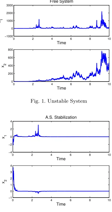
Before we proceed to study more general problem, let us discuss an example to illustrate our theory so far. Example 1. Consider a 2-dimensional linear system

dx(t) =Ax(t)dt+C1x(t)dw1(t), (17)

where

A= 3 1 0 1

!

, C1=

3 0.2 0 1

!

.

It is easy to show that this system is a.s. unstable (Fig.1). Assume that we are required to define a state-feedback controlu(t) =BKx(t) only in the shift part so that the corresponding controlled system

dx(t) = [A+BK)x(t)dt+Cix(t)dw1(t) (18)

becomes a.s. stable, where B = (1,0)T _{is given while}

K∈R1×2

is to be designed. However, given the structure of B, it is easy to see there is no suchK for equation (18) to be a.s. stable, sincex2(t) obeys

dx2(t) =x2(t)dt+x2(t)dw1(t)

whencex2(t)→ ∞a.s.

Let us now further consider the stochastic controlled system

dx(t) = (A+BK)x(t)dt+ (Ci+D1K)x(t)dw1(t), (19)

whereD1= (−1,2)T. Noting thatdEx2(t)/dt=Ex2(t),

we observe thatEx2(t)→ ∞ast→ ∞for anyx2(0)6= 0

0 2 4 6 8 10 −1000

0 1000 2000 3000

Time x1

Free System

0 2 4 6 8 10

0 200 400 600 800

[image:5.612.63.254.25.385.2]

Time x 2

Fig. 1. Unstable System

0 2 4 6 8 10

−4 −2 0 2 4

Time x1

A.S. Stabilization

0 2 4 6 8 10

−1 0 1 2 3 4

Time x2

Fig. 2. a.s. Stabilisation

in mean-square sense. However, by settingh = 1, and solving LMIs (14a) and (14b) forα=h,2h,· · ·, we find

α= 15, X = 0.3786 −0.0153

−0.0153 0.1770 !

andY = (0.0290, 0.1886). By Theorem 2 we can con-clude that chosing

K= (0.1203,1.0760)

we make system (19) a.s. stable (Fig.2).

4 Stabilization of Uncertain Systems

Let us now generalise our theory to cope with the uncer-tainty of system parameters. More precisely, let us

con-sider the uncertain stochastic control system of the form

dx(t) = [(A+ ∆A)x(t) + (B+ ∆B)u(t)]dt

+

m

X

i=1

[(Ci+ ∆Ci)x(t)

+ (Di+ ∆Di)u(t)]dwi(t), (20)

with the state-feedback control u(t) = Kx(t). The closed-loop system is

dx(t) = (A+ ∆A+ (B+ ∆B)K)x(t)dt

+

m

X

i=1

(Ci+ ∆Ci+ (Di+ ∆Di)K)x(t)dwi(t). (21)

HereA, Betc. are the same as before while the uncertain matrices are assumed to have the following structures

∆A=N0F0NA, ∆B=N0F0NB,

∆Ci=NiFiNCi, ∆Di=NiFiNDi

fori= 1,2,· · · , m, whereN0, NA, NB, Ni, NCi, NDi are

known real constant matrices with appropriate dimen-sions but Fi’s are unknown and obeyFiTFi ≤I. Such

structure uncertainty has been used by many authors e.g. Wang, Qiao & Burnham (2002); Xu & Chen (2002).

The following theorem provides an LMI method to de-sign a robust controller to stabilize the uncertain system almost surely.

Theorem 3. The equilibrium of the uncertain stochas-tic system (21) is almost surely exponentially stable with respect to state-feedback gain K = Y X−1

, if there ex-ists a positive definite matrixX, a matrixY and positive scalars αi,γ,εi,δi (i = 1,2,· · ·, m) such that the

fol-lowing LMIs hold:



     

Π11−αX ∗ ∗ ∗

NAX+NBY −γI ∗ ∗

Π31 0 Π33 ∗

Π41 0 0 Π44



     

<0 (22a)

and, for eachi= 1,2,· · ·, m, either

Ωi−δiNiNiT −

√

2αiX ∗

(NCiX+NDiY)

T _δ iI

!

>0, (22b)

or

Ωi+δiNiNiT +

√

2αiX ∗

(NCiX+NDiY)

T

−δiI

!

<0, (22c)

whereα=Pm

i=1αi,

Π11= (AX+BY)T + (AX+BY) +γN0N0T,

Π31 = [(C1X +D1Y)T,(C2X+D2Y)T,· · · ,(CmX +

[image:5.612.321.550.448.635.2]

Π33=diag(ε1N1N1T−X, ε2N2N2T−X,· · ·, εmNmNmT−

X),

Π41= [(NC₁X+ND₁Y)T,(NC₂X+ND₂Y)T,· · · ,(NCmX+

NDmY)

T_]T_,

Π44=diag(−ε1I,−ε2I,· · · ,−εmI),

Ωi= (CiX+DiY)T+CiX+DiY.

Proof. The proof is similar to that of Theorem 2 so we only give an outlined one. SetP =X−1

and letV(x) =

xT_{P xwhich obeys (9a). It is easy to show that}

LV(x) =xT_[(A+BK+N

0F0(NA+NBK))TP

+P(A+BK+N0F0(NA+NBK))]x

+xT_[ m

X

i=1

(Ci+DiK

+NiFi(NCi+NDiK))

T_P(C

i+DiK

+NiFi(NCi+NDiK))]x.

By the fundamental matrix inequalities (see e.g. Wang, Qiao & Burnham (2002); Xu & Chen (2002)), we can get

LV(x)≤xT_[(A+BK)T_{P+P(A+BK)) +γP N}

0N0TP

+ (NA+NBK)T(NA+NBK)/γ]x

+xT

m

X

i=1

[(Ci+DiK)T(X−εiNiNiT)−

1

(Ci+DiK)

+ (NCi+NDiK)

T

(NCi+NDiK)/εi]x

From this we can show in the same way as in the proof of Theorem 2 that LMI (22a) implies inequality (9b) with

c2< α. Moreover, we have

(HV(x))2

=

m

X

i=1

xT_[(C

i+DiK)TP +P(Ci+DiK)

+ (NiFi(NCi+NDiK))

T_P

+P(NiFi(NCi+NDiK))]x

2

.

For eachi= 1,2,· · · , m, it is easy to show

−δiP NiNiTP−(NCi+NDiK)

T

(NCi+NDiK)/δi ≤NiFi(NCi+NDiK))

T_P+P(N

iFi(NCi+NDiK) ≤δiP NiNiTP+ (NCi+NDiK)

T

(NCi+NDiK)/δi.

From these we can show in the same way as in the proof of Theorem 2 that (9c) withc3= 2αis guaranteed by (22b)

or (22c). Hence the assertion of this theorem follows from Lemma 1.

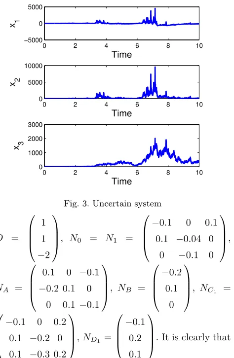
Example 2. Consider system (20) with m = 1 and

A= 

  

−1 2 0 1 3 1

0 0 1 

  

, B =     1 1 0    

, C = 

  

−2 −1 −1

−1 −3 −0.2

0 0 −1



   ,

0 2 4 6 8 10

−5000 0 5000

Time

x 1

0 2 4 6 8 10

0 5000 10000

Time

x 2

0 2 4 6 8 10

[image:6.612.312.549.30.393.2]

0 1000 2000 3000 Time x 3

Fig. 3. Uncertain system

D =     1 1 −2    

, N0 = N1 =



  

−0.1 0 0.1 0.1 −0.04 0

0 −0.1 0 

   ,

NA =



  

0.1 0 −0.1

−0.2 0.1 0 0 0.1 −0.1



  

, NB =



  

−0.2 0.1

0 

  

, NC₁ =



  

−0.1 0 0.2 0.1 −0.2 0 0.1 −0.3 0.2



  

,ND₁ =



  

−0.1 0.2 0.1



  

. It is clearly that

this system cannot be stabilised in mean-square sense. However, setting h = 1, and for α = α1 = h,2h,· · ·,

solving LMIs (22a) and (22b) we find the feasible solu-tion for the a.s. stability:

α= 20, X = 

  

1.4076 2.6818 −0.7770

2.6818 5.6305 −2.0732

−0.7770 −2.0732 6.6563 

  

,

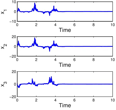
K= (−4.63862.73831.5736), γ= 5.5793, ε1= 0.8032, δ1=

3.4642. The corresponding simulation results shown in Fig.3 and Fig.4 support the stabilisation result.

5 Conclusion

[image:6.612.326.526.453.500.2]

0 2 4 6 8 10 −10

0 10

Time

x 1

0 2 4 6 8 10

−20 0 20

Time

x 2

0 2 4 6 8 10

−20 0 20

Time

[image:7.612.58.256.34.222.2]

x 3

Fig. 4. Robust a.s. Stabilization

Acknowledgements

The authors would like to thank the referee and the as-sociated editor for their helpful comments and sugges-tions. This work is supported by Royal Society / KC Wong Fellowship (UK) under Grant RD3485.

References

Arnold,L., Crauel, H., & Wihstutz, V. (1983). Stabiliza-tion of linear systems by noise.SIAM J. Control. Op-tim, 21(3), 451–461.

Appleby, J.A.D., & Mao, X. (2005). Stochastic stabili-sation of functional differential equations.Systems & Control Letters, 54(11), 1069–1081.

Boyd,S., El Ghaoui,L.,Feron E., & Balakrishnan, V.(1994). Linear Matrix Inequalities in Systems and Control Theory, Philadelphia, PA, USA: SIAM. Caraballo, T. , & Robinson, J.C. (2004). Stabilisation of

linear PDEs by Stratonovich noise.Systems & Control Letters, 53(1), 41–50.

Chen, B.-S. & Zhang, W. (2004). Stochastic H2/H∞

control with state-dependent noise. IEEE Transac-tions on Automatic Control, 49(1), 45 – 57.

Deng, H., & Krstic, M.(1997). Stochastic nonlinear stabilization—Part I: A backstepping design.Syst. Control Lett., 32, 143–150.

Dragan,V., Morozan,T., & Stoica, A. (2004).H2

Opti-mal control for linear stochastic systems.Automatica, 40, 1103–1113.

El Ghaoui, L. (1995). State-feedback control of systems with multiplicative noise via linear matrix inequali-ties.Systems & Control Letters, 24(3), 223–228. Ezzine,J.,& Kavranoglyu,D.(1997). On almost-sure

sta-bilization of discrete-time jump parameter systems: an LMI approach.Int. J. Control, 68(5),1129–1146. Fang, Y.(1997). A new general sufficient condition for

almost sure stability of jump linear systems. IEEE Trans. Automatic Control, 42(3), 378–382.

Fang, Y., & Loparo,K. A. (2002).Stabilization of continuous-time jump linear systems.IEEE Trans. Automatic Control, 47(10), 1590–1603.

Fernholz, R., & Karatzas, I. (2005). Relative arbitrage in volatility-stabilized markets,Annals of Finance, 1(2), 149 – 177.

Hinrichsen, D., & Pritchard,A.J. (1998). StochasticH∞_.

SIAM J. Control Optim., 36, 1504–1538.

Khasminski, R. Z.(1980). Stochastic stability of Differ-ential Equations, Rockville, Maryland: S&N Interna-tional Publisher.

Kwieci´nska, A. (2002). Stabilization of evolution equa-tions by noise,Proceedings of Amarican Mathematical Society, 130(10), 3067–3074.

Lee,J.W., & Dullerudb,G. E.(2006). Uniform stabiliza-tion of discrete-time switched and markovian jump linear systems.Automatica, 42, 205 – 218.

Mao X.(1997).Stochastic Differential Equations and Ap-plications, Chichester, England, UK: Horwood Pub-lishing.

Mao, X.(1994). Stochastic stabilization and destabiliza-tion.Syst. Control Lett., 23,279–290.

Nolan, V. J., & Sri Namachchivaya, N.(1999). On almost-sure stability of linear gyroscopic systems. Journal of sound and vibration, 227(1), 105–130. Pan, Z., & Basar ,T. (1999). Backstepping controller

design for nonlinear stochastic systems under a risk-sensitive cost.SIAM J. Control Optim., 37 (3), 957– 995.

Pardoux, E., & Wihstutz,V. (1992). Lyapounov expo-nent of linear stochastic systems with large diffusion term.Stochastic Processes and their Applications, 40, 289–308.

Roberts, J. B., & Spanos, P. D. (1986). Stochastic av-eraging: An approximate method of solving random vibration problems.Internat. J. Non-linear Mesh, 21, 111–134.

Tylikowski, A.(2005). Stabilization of beam parametric vibrations with shear deformations and rotary inertia effects international.Journal of solids and structures, 42, 5920–5930.

Wang,Z., Qiao,H., & Burnham,K.J.(2002). On stabi-lization of bilinear uncertain time-delay stochastic systems with Markovian jumping parameters.IEEE Trans. Automat. Contr., 47, 640 – 646.

Xu,S.,& Chen,T.(2002). RobustH∞ control for uncer-tain stochastic systems with state delay.IEEE Trans. Automat. Contr., 47, 2089-2094.

Xu,S., Shi,P., Chu, M.,& Zou,Y.(2006). Robust stochas-tic stabilization andH∞control of uncertain neutral stochastic time-delay systems.Journal of Mathemat-ical Analysis and Applications, 314(1), 1–16.

Yuan,C., & Mao, X.(2004). Robust stability and control-lability of stochastic differential delay equations with Markovian switching.Automatica, 40, 343–354. Yuan,C., & Lygeros,J.(2005) On the exponential

Au-tomatic Control, 50(9),1422–1426.