The Market Timing Ability of UK Equity Mutual Funds

City, University of London Institutional Repository

Citation:

Cuthbertson, K., O'Sullivan, N. and Nitzsche, D. (2007). The Market Timing Ability of UK Equity Mutual Funds. SSRN.

This is the published version of the paper.

This version of the publication may differ from the final published

version.

Permanent repository link:

http://openaccess.city.ac.uk/16851/

Link to published version:

Copyright and reuse: City Research Online aims to make research

outputs of City, University of London available to a wider audience.

Copyright and Moral Rights remain with the author(s) and/or copyright

holders. URLs from City Research Online may be freely distributed and

linked to.

City Research Online: http://openaccess.city.ac.uk/ [email protected]

Keith Cuthbertson*, Dirk Nitzsche* and

Niall O’Sullivan**

This version : 18th November 2006

Abstract:

We apply a recent nonparametric methodology to test the market timing skills of UK equity mutual funds. The methodology has a number of advantages over the widely used regression based tests of Treynor-Mazuy (1966) and Henriksson-Merton (1981). We find a relatively small number of funds (around 1.5%) demonstrate positive market timing ability at a 5% significance level, while around 10-20% of funds exhibit negative (perverse) timing and most funds do not time the market. Our findings indicate that the few skillful market timers possess private market timing signals so their performance cannot be attributed to publicly available information. In terms of fund classifications, there are a small number of successful positive market timers amongst equity income and general equity funds, while a few small company funds time a small company rather than a broad market index. We also apply regression based tests of volatility timing and find evidence that a slightly larger (around 5%) of funds successful time market volatility.

Keywords : Mutual funds performance, market timing.

JEL Classification: C14, G11

* Cass Business School, City University, London

** Department of Economics, University College Cork, Ireland

Corresponding Author : Professor Keith Cuthbertson

Cass Business School, City University London 106 Bunhill Row, London, EC1Y 8TZ.

Tel. : +44-(0)-20-7040-5070 Fax : +44-(0)-20-7040-8881

E-mail : [email protected]

1. Introduction

The question of market timing has attracted relatively little attention among studies of UK fund performance. One form of market timing is tactical asset allocation which keeps the composition of a portfolio of risky assets constant but alters the proportion of the portfolio held in cash (non-risky assets) according to the expected future direction of the market. Market timing may also be achieved by using index futures or other derivate positions.1 _{Alternatively, market}

timing may be implemented by rebalancing the fund’s equity holdings to increase (decrease) the fund’s market beta in response to an expected bull (bear) market. To test tactical asset allocation requires information on a portfolio’s composition over time and such data are not readily available for UK mutual funds. However, tests of whether the portfolio beta is conditional on a market benchmark may be conducted with available fund and market returns data.

In this paper we apply regression approaches and, for the first time on UK data, a nonparametric test to examine the market timing performance of individual UK domestic equity funds. Our large survivorship-bias free data base of around 800 (non-tracker, non second-unit) funds is also the most comprehensive used to-date and we extend the data set from the mid-1990s to include the market downturn after 2000.

The nonparametric procedure has several advantages. First, it measures the quality of a fund manager’s timing information rather than the aggressiveness of his response - whereas the widely used regression based methods of Treynor-Mazuy (TM) (1966) and Henriksson-Merton (HM) (1981) cannot separate these two elements. The quality of timing information is of more interest to the investor as he can control the aggressiveness of his position himself simply by adjusting his holdings of risky/non-risky assets. In addition, the nonparametric method requires less restrictive behavioural assumptions and unlike the TM and HM tests which assume the fund’s timing frequency is fixed at the same frequency as sampling interval in the data set used, the non-parametric approach is flexible in this respect. This raises a question concerning the power of different tests for market timing when actual fund timing frequencies differ from data sampling frequencies, and this is discussed further below (Goetzmann et al 2000, Bollen and Busse 2001). Furthermore, in this paper we also examine whether mutual fund managers can improve investor returns based on the quality of the manager’s private market timing information (timing signals) rather than simply relying on publicly available information (Becker et al 1999, Ferson and Khang 2001).

The performance of actively managed mutual (and other) funds, in particular relative to passive funds, is central to recent policy debates. An important question is whether voluntary saving in mutual and pension funds will be sufficient to meet a predicted future savings gap given both projected state pensions and increasing longevity, (Turner 2004, OECD 2003). It is important to evaluate the relative performance of UK actively managed funds to determine the

extent to which such funds truly add value to investors/savers as a means of efficiently allocating their scarce resources to saving instruments for the future. Recent studies have examined this question in relation to security selection skill, usually measured by a fund’s alpha (Keswani and Stolin 2005, Fletcher and Forbes 2002, Quigley and Sinquefield 2000, Cuthbertson, Nitzsche and O’ Sullivan 2005) - here we assess fund’s market timing skills.

The paper proceeds as follows. In section 2 we survey recent findings in the market timing literature. The nonparametric testing methodology is presented in section 3. In section 4 we describe the UK data set, empirical results are reported in section 5 and section 6 concludes.

2. Recent Literature

Two widely applied models of market timing are Treynor and Mazuy (1966) and Henriksson and Merton (1981), henceforth TM and HM respectively. The TM test specifies a quadratic regression of the form

(1) r_i,t+1=α_i+θ_{i m,t+1}(r )+γ_{iu m,t+1}(r ) +2 ε_i,t+1

where the coefficient γ_iu measures market timing ability. r_i,t+1 and r_m,t+1 are the fund and market

excess returns respectively. Admati et al (1986) demonstrate that the model is consistent with a

manager with constant absolute risk aversion whose beta at time t is a linear function of r_m,t+1. The

null hypothesis of no market timing implies γ_iu= 0. In the HM model the conditional portfolio beta

follows a binary response function depending on the manager’s forecast of whether next period’s market return will exceed the risk free rate. The authors show that if the manager can successfully time the market then the coefficient γ_iuin (2) will be positive.

(2) +

i,t+1 i i m,t+1 iu m,t+1 i,t+1

r =α +θ(r )+γ (r ) +ε

where (r_m,t+1)+is defined as max(0,r_m,t+1). Here max(0,r_m,t+1) may also be interpreted as the payoff

to an option on the market portfolio with a strike price equal to the risk free rate. Based on similar models, Ferson and Schadt (1996) control for timing skills which may be attributable to public information by specifying the portfolio beta to be a function of a set of relevant public information variables. The null is then a test of the quality of the fund manager’s private timing signal2.

Several difficulties may arise with the TM and HM tests. Breen at al (1986) using simulation techniques note that the HM test (which ignores heteroscedasticity) is poor both in terms of size and power. 3 A further difficulty with the TM and HM tests concerns their inability to decompose overall fund abnormal performance into its market timing and security selection

2

See also Becker et al (1999) and Ferson and Khang (2001) for further discussion on the effects of conditioning information on timing performance measures. Portfolio managers may also adjust a fund’s exposure to risk factors other than the market or indeed to other benchmark indices according to their year-to-date performance in response to incentives they may face (Chevalier and Ellison, 1997; Brown, Harlow and Starks, 1996).

components, (Admati et al 1986, Grinblatt and Titman 1989). Many studies point to a negative correlation between the market timing and selectivity measures of performance (Jagannathan and Korajczyk 1986, Coggin et al 1993, Goetzmann et al 2000, Jiang 2003). For example, simulations in Jiang (2003) show a negative correlation between the two performance measures in the TM and HM models, even where none exists, whereas the correlation between the nonparametric timing measure and the security selection measure in the regression models is very small (indistinguishable from zero for larger sample sizes). Jagannathan and Korajczyk (1986) suggest that a spurious negative correlation may arise due to the nonlinear pay-off structure of options and option-like securities in fund portfolios. Holding a call option on the market yields a high pay-off in a rising market but in a steady or falling market the premium payment lowers return and appears as poor security selection4_{. However, using (quarterly) holdings data Jiang, Yao and Yu (2005)}

apply a methodology which controls for this option effect and find significant timing ability among some US mutual funds using monthly returns.

A further difficulty in assessing fund timing ability arises if the frequency of the researcher’s observed data differs from the frequency of the manager’s timing strategy (where the latter may not be uniform or even known). Using standard regression tests for market timing and a bootstrap simulation technique, Bollen and Busse (2001) generate synthetic fund returns which mimic the holdings of actual funds using both daily and monthly data and show that while the tests for market timing on daily data yield expected results, the results using monthly data are biased. Then using actual daily data, Bollen and Busse provide stronger evidence of positive market timing ability than when using actual monthly data. Goetzmann et al (2000) similarly demonstrate that the HM test is biased downwards when applied to the monthly returns of daily timers. Bollen and Busse (2005) is the only study to examine persistence in market timing and finds evidence of short term persistence when using daily data.

The bulk of the US empirical evidence on market timing demonstrates no market timing or perverse negative market timing (Wermers 20005_{, Ferson and Schadt 1996, Becker at al 1999,}

Goetzmann et al 2000; Jiang, 2003) - although conditioning on public information is shown to improve the model specification (Ferson and Warther 1996, Ferson and Schadt 1996, Becker at al 1999). Mamaysky, Spiegel and Zhang (2004) use the Kalman filter to model time varying betas (and alphas). With dynamic estimates the authors explore which trading strategies are associated with outperformance. The findings indicate that superior and inferior returns are linked to attempts at market timing rather than stock selection, though in aggregate there is little evidence that investors earn superior returns.

A possible explanation of poor market timing may lie in mutual fund cashflows (Bollen and Busse 2001, Edelen 1999, Warther 1995, Ferson and Warther 1996). Investors increase net

4

The returns on the common stock of highly geared firms may create a similar effect. Thus portfolios heavily weighted in highly (lowly) geared stocks such as small stocks (blue chips) may appear to exhibit stronger (weaker) market timing effects. This may account for the predominant finding of poor or even negative market timing in the literature.

5

cashflows into mutual funds during periods when the market return is relatively high, increasing the fund’s cash position, causing a concurrent lower overall portfolio return. As noted by Bollen and Busse (2001), in the HM model the market timing coefficient is estimated only when the market (excess) return is positive and so the cash-flow hypothesis is asymmetric: it can bias the coefficient downwards but not upwards. The authors also argue that the timing coefficient in the TM test is similarly biased downward.

A further question in the market timing literature is that of volatility timing. If market return and market volatility are unrelated, fund managers may be able to enhance investor utility by reducing market exposure when conditional volatility is high. The latter is often predictable since it persists: periods of high (low) volatility are often followed by high (low) volatility6_{. Busse (1999) has}

shown that US funds do attempt to reduce market exposure when market volatility is high. However, if market return and volatility are positively related then attempts to time volatility may appear as negative market timing. In this paper, we also test for volatility timing as well as joint return and volatility timing.

Overall using standard parametric tests, US daily data provides some evidence of successful market timing but when using monthly data successful market timing seems weak or non-existent. Jiang (2003) proposes a nonparametric test of market timing in order to address some of the issues above and this methodology is described in section 3.

While there have been several recent studies on the ex-ante performance and performance persistence of UK funds (Fletcher and Forbes 2002, Keswani and Stolin 2005, Otten and Bams 2002, Quigley and Sinquefield 2000, Blake and Timmermann 1998), there has been relatively little research carried out on the market timing skills of UK equity unit and investment trusts. Fletcher (1995) applies both the Chen and Stockum (1986) (similar to TM) and HM timing tests. Evaluating 101 unit trusts between 1980 and 1989, Fletcher reports the cross sectional average timing measures to be negative and strongly significant. This is found to be the case for both models of market timing and alternative market benchmark indices. Leger (1997) evaluates UK equity investment trusts between 1974 and 1993 and finds similar results - negative and statistically significant market timing.

3. Nonparametric Test of Market Timing

Because of the difficulties noted above with regression based tests of market timing, Jiang (2003) uses a non-parametric test on US mutual funds, which we outline below. The market model is:

(3) r_i,t+1=α_i+β_{i,t m,t+1}r +ε_i,t+1

where r_i,t+1 is the excess return on fund i, r_m,t+1 is the relevant benchmark market excess return

against which the fund is evaluated, α_i is a security selectivity measure (assumed to be

independent of market timing) and the fund’s betaβ_i,t is assumed to vary with the fund manager’s

market timing information at time t. The fund’s timing skill is determined by the ability to correctly predict market movements. Let _rˆ_{m,t+1= E(rm,t+1| I )t be the manager’s forecast for the next period’s}

market return based on the information set I_t. The parameter vis defined as

(4) ˆ ˆ ˆ ˆ

2 1 2 1 2 1 2 1

m,t +1 m,t +1 m,t +1 m,t +1 m,t +1 m,t +1 m,t +1 m,t +1

v = Pr(r > r | r > r ) -Pr(r < r | r > r )

Under the null hypothesis of no market timing ability v = 0 since the probability of a correct forecast then equals the probability of an incorrect forecast. ν∈[-1,1] where the two extreme values represent perfect negative and perfect positive (i.e. successful) market timing respectively. Equation (4) may also be written as:

(5) ˆ ˆ

2 1 2 1

m,t +1 m,t +1 m,t +1 m,t +1

v = 2Pr(r > r | r > r ) -1

The next step is to link the manager’s forecast of the market return with his response in adjusting β_i,t in (3). For any triplet of market return observations

1 2 3

m,t m,t m,t

{r ,r ,r }sampled from any

three time periods (not necessarily in consecutive order) with

1 2 3

m,t m,t m,t

{r < r < r } an informed

market timer will maintain a higher exposure to the market over the

2 3

m,t m,t

[r ,r ]range than in

the

1 2

m,t m,t

[r ,r ] range. Nonparametric beta estimates for both time ranges are

1 2 1 2 1

t i,t i,t m,t m,t

β = (r - r )/(r - r ) and β_t2 = (r_i,t3 - r )/(r_{i,t2 m,t3}- r_m,t2). Here beta embodies both the precision

of the market return forecast and the aggressiveness of the manager’s response where the latter is affected by risk aversion. Grinblatt and Titman (1989) show that for a fund i with non-increasing

absolute risk aversion and independent timing and selectivity information

ˆ t m,t+1 β > 0 r δ

δ yielding a

convex fund return/market return relationship

(6) 3 2 2 1

3 2 2 1

i,t i,t i,t i,t m,t m,t m,t m,t

r - r r - r

>

r - r r - r

which allows (5) to be written as v = 2Pr(β_t2 >β_t1| r_{m,t +12} > r_{m,t +11} ) -1. A sample statistic of a fund’s

timing ability may be constructed as:

(7) ˆ 3 2 2 1

3 2 2 1

m,t1 m,t2 m,t3

-1

i,t i,t i,t i,t n

m,t m,t m,t m,t r <r <r

r - r r - r

n

θ = sign >

3 r - r r - r

⎛ ⎞

⎛ ⎞

⎜ ⎟

⎜ ⎟ _{⎜ ⎟}

where sign (⋅) = (1, -1, 0) for positive, negative and zero market timing respectively. ˆ

n

θ is the

average sign across all triplets taken from n observations and is a U-statistic with kernel of order

three. ˆ

n

θ can be shown to be √n-consistent and asymptotically normal (Abrevaya and Jiang 2001,

Serfling 1980) with variance:

(8) ˆˆ _{1 2 3} ˆ

n

1 2 3 1 2 1 3

2 -1

n 2

t t t n

θ

t =1 t <t ,t ¹t ,t ¹t

n 9

σ = h(z ,z ,z ) -θ

2 n ⎛_{⎛ ⎞} ⎞ ⎜_{⎜ ⎟} ⎟ ⎜_{⎝ ⎠} ⎟ ⎝ ⎠

∑

∑

where

(9) 3 2 2 1

1 2 3 1 2 3

3 2 2 1

, , , ,

, , , , , , ,

(

t

,

t

,

t

)

i t i t i t i t

|

m t m t m t

m t m t m t m t

r

r

r

r

h z z

z

sign

r

r

r

r

r

r

r

⎛

−

−

⎞

=

⎜

_⎜

>

<

<

⎟

_⎟

−

−

⎝

⎠

Under the null hypothesis of no market timing ˆ ˆˆ

n

n _θ

z = n.θ σ is asymptotically N(0,1).

Note, the calculation in (9) includes triplets h(z ,z ,z ), h(z ,z ,z ), h(z ,z ,z )_{t1 t2 t3 t2 t1 t3 t3 t1 t2} , that is the

same three market return observations drawn in different combinations. However, the sign in (10) is equal in all three cases since it is conditional on r_m,t1< r_m,t2 < r_m,t3. That is, irrespective of the

order in which the market return observations are drawn they are first sorted in ascending order and there can only be one such sorting.

As discussed, one difficulty in examining a fund’s market timing skill is decomposing the quality of the manager’s information regarding the future market return and the aggressiveness of his response in changing the fund’s beta. A rational investor is more concerned with the former as he can control the latter himself by choosing the proportion of his wealth to invest in the fund. The TM and HM market timing measures test for both information quality and aggressiveness of response and hence such tests cannot separate out the two effects. For example, Henriksson-Merton (1981) show that (p +p -1).(_{1 2} η₂-η₁)is a consistent estimate of γ_iu in (2) where p₁ and p₂

are the conditional probabilities of the manager correctly forecasting negative and positive market excess returns respectively in period t+1 and η₁ and η₂are the fund target betas in each case.

Hence the estimated HM timing measure in (2) incorporates both the quality of manager information, p +p -1_{1 2} , and the aggressiveness of response, η₂-η₁. The nonparametric measure

on the other hand simply measures how often a manager correctly forecasts a market movement and acts on it - irrespective of how aggressively he acts on it. This is reflected in the fact that the sign function in (8) assigns a value of 1(-1) if the argument is positive (negative) regardless of the size of the argument.

timing over all triplets of fund returns rather than just consecutive observations and consequently uses more information than parametric tests. Therefore, the nonparametric measure permits the cross-section of fund managers to have different timing frequencies whereas the regression based approaches of TM and HM are more restrictive since they assume the timing frequency of each manager is known and that this (on average) is the same across managers.

However, the nonparametric test also embodies some relatively mild restrictions on behaviour. First, the test requires β_t be a non-decreasing function of ˆ_{rm,t+1. Grinblatt and Titman}

(1989) demonstrate that this requires (i) non-increasing absolute risk aversion, (ii) independently and identically distributed (iid) market returns and (iii) independent selectivity and timing information. First, the requirement of non-increasing absolute risk aversion is less restrictive than that of the TM and HM measures which require specific linear and binary response functions respectively. For example, the linear response function embodied in the TM measure is consistent with the manager maximising a Constant Absolute Risk Aversion (CARA) preference function (Admati et al, 1986). However, such an assumption is questionable if there is non-linearity in the payment to fund managers in respect of benchmark evaluation (Admati and Pfleiderer, 1997), option compensation (Carpenter, 2000) and a non-linear performance-flow responses by investors (Chevalier and Ellison, 1997). Second, the iid assumption rules out heteroscedasticity in market returns and hence volatility timing by fund managers – but empirically this effect appears to be weak (Busse 1999). Third, distinguishing between timing and selectivity skill in the attribution of performance is difficult empirically though independent selectivity and timing information is a common assumption (see Admati et al 1986, Grinblatt and Titman 1989). As discussed previously, Jagannathan and Korajczyk (1986) question this assumption with respect to options and option-like securities with nonlinear pay-offs. The non-parametric measure, option-like that of TM and HM, cannot distinguish between market timing and spurious option related effects. However, all funds examined in this study are comprised of at least 80% UK domestic equity (typically funds hold an even higher percentage) so any distortion due to holding options is likely to be relatively small7.

Finally, the HM regression approach suffers size and power distortion under heteroscedasticty but the asymptotic distribution of the nonparametric timing measure in (8) is unaffected by heteroscedasticity in fund returns.

Conditional Market Timing: Public versus Private Information

The nonparametric test can be applied as a conditional statistic after allowing for market timing skill attributable to public information. This conditional measure involves first calculating both sets of residuals from regressions of the mutual fund returns and market returns on the lagged public information variables. Clearly, these residuals represent the variation in the fund and market returns not explained by the public information. Denote the pairwise fund and market

7

regression residuals as r%_i,tand r%_m,t respectively. The procedure described above in (8) may then

be applied to the residuals to yield a conditional timing measure

(10) 3 2 2 1

3 2 2 1

m,t1 m,t2 m,t3

-1

i,t i,t i,t i,t n

m,t m,t m,t m,t r <r <r

r - r r - r

n

θ = sign >

3 r - r r - r

⎛ ⎞ ⎛ ⎞ ⎜ ⎟ ⎜ ⎟ _{⎜ ⎟} ⎝ ⎠ _{% %}

∑

_{% ⎝ ⎠} % % % % % % % % %

Note, ˆ

n

θ in (8) and θ%_nin (11) can clearly be of different magnitudes but may also be of

different sign. For example, ˆ

n

θ > 0 but θ%_n< 0may indicate a successful market timing manager

whose skill is attributable to public information.

We examine conditional market timing using a set of public information variables which may provide market return predictability (Ferson and Schadt 1996). They include (i) the one month UK Tbill rate, (ii) the market divided yield, (iii) the term spread (20 year – 1 month yields) and (iv) the gilt/equity yield ratio. The gilt/equity yield ratio is the ratio of the coupon yield on a long term government bond to the market dividend yield. It captures the relative attractiveness of bonds versus equity and as such may help predict returns in both markets, (Clare, Wickens and Thomas 1994). We use the yield on a 30 year UK government bond.

Volatility Timing

In addition to timing the market return, fund managers may also attempt to time volatility in the market return - ceteris paribus, the manager will reduce market exposure in anticipation of higher (conditional) volatility. Expressing the fund beta as a linear function of market (demeaned) volatility gives (Busse 1999):

(11)

k

i,t+1 j j,t+1 m,t+1 m,t+1 m t+1 j=1

r =α+

∑

βr +λr (σ -σ ) +ε

where σ_m,t+1represents market volatility. Similar to Busse (1999) we estimate conditional volatility

as8 (12) t 1 n 2 2 mt mti mt

i=1

σ =⎡⎢ (r - r ) ⎤⎥

⎢ ⎥

⎣

∑

⎦

where r_mtiare the nt daily market returns during month t and rj,t+1 (j = 1,2..k) are risk factors in the

equilibrium model of security returns. Successful volatility timing is indicated by a negative value of

λin (11).

Fund managers may also pursue a strategy of jointly timing both the level and the volatility of the market portfolio. Writing beta as a linear function of both market return and volatility yields a return-volatility timing model of the form:

(13)

k

2

i,t+1 j j,t+1 m,t+1 m,t+1 m,t+1 m t+1 j=1

r =α+

∑

βr +γr +λr (σ -σ ) +ε

where γ > 0and λ< 0measure successful market return and volatility timing respectively.

Alternatively, to jointly test market return and volatility timing Chen and Liang (2006) propose a model of the form

(14)

2 k

m,t+1

i,t+1 j j,t+1 t+1 m,t+1

j=1

r

r =α+ βr +γ +ε

σ

⎛ ⎞

⎜ ⎟

⎜ ⎟

⎝ ⎠

∑

where the coefficient γ on the square of the conditional Sharpe ratio of the market portfolio has

the intuitive appeal of measuring the manager’s ability to time periods of high market return relative to volatility. Here such successful timing is indicated byγ> 0. We estimate these three

models of market timing.

4. Data

Our mutual fund data set contains monthly returns on 842 (actively managed) UK equity Unit Trusts and Open Ended Investment Companies. ‘UK Equity’ funds (by definition) have at least 80% of the fund invested in UK equity. This data set represents almost the entire set of UK equity funds which have existed at any point during the period January 1988 – December 20029. By restricting funds to those investing in UK equity, more accurate market benchmarks may be used.

The data set includes both surviving funds (626) and nonsurviving funds (216) in order to control for survivorship bias. Nonsurviving funds are those which cease to exist at some point prior to the end of the sample period. Failure to include nonsurviving funds may bias performance findings upwards if their closure is related to poor performance. Funds are also categorised by investment objectives: equity income funds (162), ‘All Company’ or ‘general equity ’ funds (553) and smaller company funds (127). In addition, funds are also categorized by the location of operation - onshore funds (662) are domiciled in the UK while offshore funds (180) are domiciled in locations such as Dublin, Luxembourg, the Channel Islands and some other European locations, although all funds are UK equity funds. Fund returns are measured before taxes on dividends and capital gains but net of management fees. Hence, we follow the usual convention in using net returns (bid-price to bid-price, with gross income reinvested). Fund ‘second units’ have

been excluded from the analysis. These arise for the most part when a single fund is sold under different pricing structures to different groups of investors such as retail and institutional or when the same fund is sold under agreed but slightly different pricing structures by life assurance companies etc. Second units do not represent separate independent portfolios and hence we exclude them. The market benchmark is the FT All Share Index of total returns (i.e. including reinvested dividends)10. Excess returns are calculated using the one-month UK T-bill rate.

5. Empirical Results

The unconditional market timing tests are presented in Table 1. Row 1 displays the market

timing test statistic, ˆ ˆˆ

n

n _θ

z = n.θ σ at various points in the cross-section of performance ranging

from the best to the worst and this is distributed asymptotically as N(0,1) under the null of no

market timing. Row 2 displays the market timing coefficient, ˆ

n

θ , corresponding to the fund in row

1.11 _{From the z-statistic in row 1, it is evident that there are only a small number of skilled market}

timers: the top 12 ranked funds demonstrate statistically significant positive market timing ability at the 5% significance level (one-tail test) – around 1.5% of the sample of funds12_{. The}

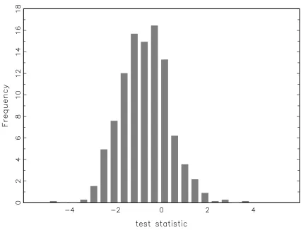
cross-sectional average test statistic is z = -0.738. More specifically, 77% of funds demonstrate negative market timing while 20% are statistically significant negative market timers. Figure 1 plots a histogram of the cross-sectional distribution of the z-statistic where it is clear the distribution is centered on a value less than zero (indicating negative market timing ability on average) with some funds in the tails exhibiting both statistically significant positive and negative market timing.

Overall, the nonparametric test fails to find evidence of timing ability among more than a ‘handful’ of UK equity mutual funds. For comparison, Table 1 (row 3 and row 4) also reports the t-statistics of the market timing coefficients of the TM and HM tests (for the funds as ranked in row 1)13. Interestingly, 10 (11) of the top 12 funds which are found to be statistically significant positive market timers using the nonparametric test are also found to be successful market timers using the TM (HM) procedure at the 5% significance level. However overall, the regression tests indicate somewhat stronger evidence of market timing than the non-parametric z-statistic, since for the TM and HM models 31 and 22 funds respectively, are found to have statistically significant positive timing skill. Correlation coefficients between the market timing test statistics of the three procedures reveals a higher coefficient of 0.95 between the TM and HM procedures than the nonparametric/TM correlation coefficient of 0.81 or the nonparametric/HM correlation coefficient of 0.86. Jiang (2003) reports similar findings and suggests that the higher correlation between the TM and HM measures may arise because these methods capture not only the quality of the fund

10 _{Results are broadly similar when we use the FT 100 index as the market benchmark.} 11

To improve statistical reliability results are reported for funds with a minimum of 12 observations which leaves 791 funds in the analysis.

12

When discussing the proportion (or total number) of funds that have a statistically significant value for z , then strictly speaking we are in a multiple testing framework so the significance level for the overall proportion of significant funds will be different from the 5% significance level for each fund taken individually (because of compound type-I errors) – see Barras et al (2005).

manager’s timing information but also the aggressiveness of response - the nonparametric measure, on the other hand, is unaffected by the aggressiveness of response. This methodological difference may also account for the slightly higher prevalence of positive timing found by the TM and HM methods relative to the nonparametric procedure.

To mitigate survivorship bias we include nonsurviving funds in the analysis14. Of the 791 funds examined, 208 are nonsurvivors. In Table 1, the row denoted ‘Survival’ indicates whether the ranked funds were survivors or nonsurvivors: 1 denotes a survivor, 0 a nonsurvivor. None of the funds which demonstrate statistically significant positive timing ability are nonsurvivors and of the top 20 ranked funds only one is a nonsurvivor. However, nonsurviving funds are not notably bad market timers.

Our (unconditional) market timing results for UK mutual funds are broadly in line with those of Jiang (2003) for the US who reports that between 2% and 5% of funds possess statistically significant positive timing skill (depending on the alternative market indices used) and also reports that the average US fund displays negative timing ability. To examine the question of whether market timing ability is related to the age of the fund, the final row of Table 1 reports the number of (monthly) observations for each of the funds. It is evident that better performing market timers are generally shorter-lived funds15_.

Market Timing Performance by Investment Style and Location

To explore possible differences in timing skill between funds of different investment objectives, i.e. income funds, general equity funds, small stock funds, we present more detailed results by investment objective in Table 2. However, there is some potential for spurious timing inferences across fund investment styles. One difficulty is the assumed independence between security selection and market timing information. A manager’s information in both these areas may be correlated and consequently selectivity and market timing inferences may be difficult to ‘disentangle’ (Admati et al 1986, Grinblatt and Titman 1989). For example, it has been argued that small stock funds may exhibit spurious timing against a market benchmark comprised of large stocks as small stocks may have (call) option-like characteristics, (Jagannathan and Korajczyk, 1986). Alternatively, it may be argued that general equity funds select from the broadest universe of stocks which make up the benchmark market portfolio, again creating an overlap between selectivity and timing decisions.

Notwithstanding the above caveats, comparing row 1 of each panel in Table 2 it is clear that there is some evidence of positive market timing ability using the nonparametric z-statistic

14

However, a fund must possess a minimum of 12 monthly observations to be included in the analysis and this restriction is imposed to improve the statistical reliability of the market timing estimates.

15

both for equity income funds and general equity funds in the extreme right tails of the distribution, while no small company funds exhibit statistically significant positive market timing. For small stock funds, the average timing coefficient is z = -1.55 compared to z = -0.62 and z = -0.57 among the equity income and general equity funds respectively. This comparatively poor performance is also evident in Figure 2 which shows histograms for the performance distributions of the three investment styles - around 15% of funds in equity income and general equity and up to 47% of funds in the small company sectors show statistically significant negative timing. The results of the TM and HM regression tests point to similar conclusions on investment style and timing performance.

We next investigate whether the small company funds attempt to time a small capitalisation market benchmark rather than a broader market benchmark. In Panel C, (Table 2) the row denoted ‘HGSC’ reports the nonparametric test statistics for small company funds measured against the Hoare Govett Small Capitalisation index for UK small stocks. The cross-sectional distribution reported in this row lies further to the right of the distribution presented in row 2 using the broader FTSE All Share market returns. The z-statistics suggest that around 7 of the small company funds have some success in timing the small-cap index and the latter indicates considerably less negative market timing than does the broad market index. Broadly similar results on market timing performance by investment sector are reported for the US by Jiang (2003) who demonstrates very few significant differences in timing ability between funds of different investment objectives – and all sectors except a specialist technology sector are shown, on average, to mis-time the market.

Table 3 presents the market timing test statistics of funds categorised by the fund location. Panel A presents results for the 623 onshore UK funds while Panel B reports results for the 168 offshore funds. A small number of both onshore and offshore funds (around 1% and 2% respectively) exhibit statistically significant positive market timing (at a 5% significance level) when using the nonparametric z-statistic while among onshore funds a higher proportion of funds exhibit statistically significant negative market timing (21%) compared to 14% of offshore funds16.

Conditional Market Timing

Tests of conditional market timing can determine whether our findings of a small number of successful market timers is attributed to public information or whether it represents genuine skill in using price information. Table 4 reports the results from a selection of conditional tests using public information variables: Z1 = 1 month UK Tbill rate, Z2 = term spread, Z3 = market dividend

16

yield and Z4 = gilt/equity yield ratio.17. (The first row is taken from the unconditional tests in Table 1 for ease of comparison). The conditional test statistics correspond to the funds as ranked in row 1. The results are similar to the unconditional timing test and are largely invariant to the choice of conditioning variables, Z. Across the conditional tests there is evidence that around 7 funds (top 1%) have genuine market timing skill (with few exceptions outside the top 7). Hence we cannot reject the hypothesis that a small number of funds successfully time the market - on the other hand around 10% of funds demonstrate statistically significant negative market timing.

Volatility Timing

Funds may attempt to time market volatility as well as market return. We report results from the regression based tests of market return and volatility timing in equations (11), (13) and (14) above. Assessing volatility timing in equation (11) we find evidence that around 7% of funds successfully time volatility (at 5% significance level using a one-tail test). A test of the hypothesis of return and volatility timing (using the Sharpe ratio formulation of equation 14) reveals that only 32 funds (4%) provide evidence of skillful market timing. Finally, using the joint timing test of equation (13), we find that 25 funds positively time the market return with γ> 0 (and a subset of 9

of these funds also successfully time market volatility, λ< 0 ). Looking at the 48 funds which are successful volatility timers (λ< 0), we find a subset of 9 of these are also positive market return timers18,19.

In Table 5 we report the extent of the overlap between funds which successfully time market return by the nonparametric test and funds which successfully time market volatility by the alternative regression based tests. The table reports results for the top 12 funds sorted by the nonparametric tests statistic. (Previously, 12 funds were found to be significant positive market return timers by this test). Of the 12 positive market timers, only 1 fund is found to successfully time market volatility (row 2) but 8 funds are shown to jointly time return and volatility (row 3).

Overall, the evidence of volatility timing among UK equity mutual funds appears to be slightly more prevalent than return timing. However, we find no evidence of a positive relation between market return and volatility in the UK (the correlation between the two measures in our data is – 0.02) indicating that volatility timing does not offer an explanation for the poor market timing results20_.

17_{In results not shown, conditional tests using a number of alternative combinations of the public information variables} were applied and results are similar to those presented.

18 _{All tests use Newey-West autocorrelation adjusted standard errors.} 19

Funds which successfully time market volatility are found in all three sectors of income, general equity and small stock funds as well as both onshore/offshore and survivors/nonsurvivor funds. However, similar to the return timing results reported previously, small stock funds are slightly under-represented.

6. Conclusion

In this paper we have used standard parametric tests and, for the first time on UK data, non-parametric tests to assess the market timing performance of individual UK mutual funds. Our large survivorship free data base of around 800 (non-tracker, non second-unit) funds is also the most comprehensive used to-date and we extend the data set from the mid-1990s to include the market downturn after 2000. The non-parametric approach is less restrictive in its behavioural assumption than the standard regression based tests. It also has the advantage of being able to isolate market timing ability on the basis of the quality of the information used, from the aggressiveness with which funds switch into the market – it is the former in which investors are primarily interested, since they can determine the amount of risk capital to invest themselves after observing the ‘quality’ of the fund’s market timing.

On the basis of our non-parametric tests we find that a relatively small number (around 1.5%) of UK equity mutual funds possess significant positive market timing skill, while a larger proportion of around 20% are shown to mis-time the market. This evidence of market timing (both positive and negative) is found to be less than is suggested by the regression based approaches of Treynor-Mazuy and Henriksson–Merton and this may be because the latter tests incorporate the aggressiveness of the manager’s response to timing signals while the nonparametric measure does not. Similarly, our nonparametric results suggest that while the cross-sectional average timing measure is negative it is not significantly so but this is in contrast to previous UK studies such as Fletcher (1995) and Leger (1997) which use the regression based tests. Our nonparametric results are robust with respect to the choice of benchmark market returns against which funds are evaluated, with respect to whether timing performance is measured unconditionally or conditionally upon public information and results broadly apply to all three investment styles analysed, though small company funds are found to time a small stock index rather than a broad market index.

[image:17.595.58.790.234.378.2]

Table 1: Mutual Fund Market Timing Performance – Unconditional Tests

Table 1 presents results for the unconditional market timing tests. Row 1 reports the nonparametric test statistic, ˆ ˆ_ˆ

n

n _θ

z = n.θ σ which is asymptotically distributed as N(0,1) under the null of no

market timing skill, and funds are presented from worst to best based on this statistic. Row 2 reports θˆ_n, the market timing coefficient, for funds in row 1. Row 3 and row 4 show the t-statistics of the TM and HM timing coefficients respectively. Row 5 reports the nonparametric test statistic, z, using the FT100, rather than the FTSE All Share index, as the market benchmark. Row 6 describes the investment objective of the funds in row 1 where, 1 = equity income fund, 2 = general equity fund, 3 = small stock fund. Row 7 indicates whether the fund is a survivor or non-survivor fund: 1 = surviving fund, 0 = non-surviving fund. Row 8 describes the fund location: 1 = onshore, 0 = offshore fund. Row 9 displays the number of fund observations. Results relate to the period 1988M1:2002M12 and are restricted to funds with a minimum of 12 observations, leaving 791 funds in the analysis.

Unconditional Market Timing Results

min 5.min min5% min10% min40% max30% max10% max5% max3% 20max 15max 12max 10max 7max 5.max 3.max 2.max max

Test Stat, z. -4.927 -3.054 -2.398 -2.071 -1.026 -0.174 0.563 0.956 1.343 1.407 1.549 1.668 1.812 1.952 2.028 2.801 2.861 3.868

ˆ

n

θ _{-0.472 -0.093 -0.077 -0.063 -0.030 -0.007 0.020 0.052 0.127 0.133 0.117 0.101 0.116 0.226 0.128 0.152 0.190 0.231}

t( TM ) -6.438 -3.512 -2.179 -1.792 -1.811 -0.194 -0.330 3.280 1.957 2.394 1.796 1.032 1.119 5.996 3.128 3.025 2.848 4.318

t( HM ) -6.873 -3.569 -2.367 -1.747 -1.469 -0.580 -0.041 2.676 1.532 2.010 1.919 1.887 1.476 4.322 3.004 2.784 3.088 3.957

z (FT100) -6.120 -3.509 -2.855 -2.508 -1.570 -0.808 0.044 0.566 0.817 0.929 1.177 1.285 1.300 1.542 1.814 2.563 3.078 3.092

Style 2 2 3 3 2 2 2 2 2 2 2 2 2 2 2 2 1 1 Survival 1 1 0 1 1 1 1 1 1 0 1 1 1 1 1 1 1 1

Location 1 1 1 1 0 0 1 1 0 1 1 0 1 1 0 1 1 1

[image:18.595.98.524.153.479.2]

Figure 1: Distribution of the Unconditional Market Timing Test Statistic

[image:19.595.104.704.227.493.2]

Table 2: Mutual Fund Market Timing Performance – By Investment Style

Table 2 presents results for the unconditional market timing tests by investment style. In each panel, Row 1 reports the nonparametric test statistic,

n ˆ

n θ

ˆ _ˆ

z = n.θ σ , and the funds are presented

from worst to best based on this statistic. Row 2 reports θˆ_n, the market timing coefficient for funds in row 1. Row 3 and row 4 show the t-statistics of the TM and HM timing coefficients respectively. In Panel A, row 5 reports the nonparametric test statistic, z, using the FT100, rather than the FTSE All Share index, as the market benchmark. In Panel C, row 5 reports the test statistic, z, using the Hoare Govett Small Cap (HGSC) index as the market benchmark. In all panels, rows denoted ‘survival’ indicate whether the fund is a survivor or non-survivor fund: 1 = surviving fund, 0 = non-surviving fund. Rows denoted ‘Location’ indicates fund location: 1 = onshore, 0 = offshore fund. The final row in each panel displays the number of fund observations. Results relate to the period 1988M1:2002M12 with 155 equity income, 514 equity and 122 small stock funds.

Unconditional Market Timing – By Investment Style

Panel A : Equity Income

min 5.min min5% min10% min20% min40% max30% max20% max10% 10max 7max 5.max 3.max 2.max max

Test Stat, z -3.137 -2.275 -1.969 -1.838 -1.520 -0.898 -0.202 0.081 0.517 0.762 1.066 1.401 2.179 2.861 3.868 ˆ

n

θ _{-0.082 -0.296 -0.062 -0.051 -0.048 -0.032 -0.007 0.002 0.022 0.023 0.062 0.044 0.229 0.190 0.232}

t(TM) -3.445 -2.943 -1.832 -0.820 -3.615 -0.611 -0.383 -0.109 -0.499 -0.373 3.062 0.121 2.084 2.848 4.318

t(HM) -3.701 -3.821 -1.892 -1.250 -3.144 -0.556 -0.168 0.018 -0.513 0.056 2.669 0.481 2.090 3.088 3.957

z (FT100) -3.717 -2.855 -2.576 -2.268 -1.907 -1.528 -0.863 -0.613 -0.031 0.346 0.711 0.914 2.563 3.078 3.092

Survival 1 1 1 1 1 0 0 1 1 0 1 0 1 1 1

Location 1 1 1 1 1 1 1 1 0 1 1 1 0 1 1

No. Obs. 180 14 180 180 180 132 132 177 105 132 83 129 32 44 39

Panel B : General Equity

min 5min min5% min10% min20% min40% max30% max20% max10% 10max 7max 5max 3max 2max max

Test Stat, z -4.927 -2.875 -2.331 -1.925 -1.394 -0.821 -0.055 0.221 0.744 1.617 1.812 1.922 2.019 2.028 2.801 ˆ

n

θ _{-0.472 -0.192 -0.144 -0.156 -0.043 -0.026 -0.002 0.007 0.080 0.169 0.116 0.121 0.216 0.128 0.152}

t(TM) -6.438 -3.065 -3.486 -1.727 -2.791 -1.757 -0.232 1.183 1.249 0.395 1.119 3.766 1.742 3.128 3.025

t(HM) -6.873 -3.195 -2.473 -2.596 -2.281 -1.437 -0.204 1.134 0.904 0.549 1.476 3.049 1.924 3.004 2.784

Survival 1 1 0 1 1 1 0 0 1 1 1 1 1 1 1

Location 1 1 1 0 1 1 1 1 1 1 1 1 1 0 1

Panel C : Smaller Companies

min 5.min min5% min10% min20% min40% max30% max20% max10% 10max 7max 5.max 3.max 2.max max

Test Stat, z -3.243 -2.752 -2.658 -2.439 -2.218 -1.806 -1.258 -1.079 -0.513 -0.248 -0.055 0.072 0.573 0.683 0.983 ˆ

n

θ _{-0.094 -0.085 -0.081 -0.132 -0.066 -0.053 -0.049 -0.062 -0.042 -0.022 -0.002 0.003 0.116 0.069 0.116}

t(TM) -3.178 -2.005 -2.289 -2.262 -3.530 -1.973 -1.299 -1.018 -0.495 -0.812 -1.062 -0.641 -0.728 0.859 0.389

t(HM) -3.198 -2.491 -2.343 -1.778 -3.478 -2.130 -1.268 -1.336 -0.621 -0.723 -0.526 -0.372 -0.511 0.425 0.433

z (HGSC) -1.781 -1.445 -1.195 -0.972 -0.567 0.309 0.510 0.787 1.186 1.232 1.698 1.722 1.966 2.058 2.167

Survival 0 0 1 0 1 1 1 1 1 1 0 1 1 1 1

Location 1 1 1 1 1 1 1 1 0 1 1 1 1 0 1

[image:21.595.107.707.224.479.2]

Table 3: Mutual Fund Market Timing Performance – By Fund Location

Table 3 presents results for the unconditional market timing tests by fund location. Row 1 reports the nonparametric test statistic, ˆ ˆ_ˆ

n

n _θ

z = n.θ σ , and funds are presented from worst to best based

on this statistic. Row 2 reports θˆ_n, the market timing coefficient for funds in row 1. Row 3 and row 4 show the t-statistics of the TM and HM timing coefficients respectively. Row 5 indicates whether the fund is a survivor or non-survivor fund: 1 = surviving fund, 0 = non-surviving fund. Row 6 describes the investment objective of the sorted funds: 1 = equity income fund, 2 = general equity fund, 3 = small stock fund. Row 7 displays the number of fund observations. Results relate to the period 1988M1:2002M12 with 623 onshore and 168 offshore funds.

Unconditional Market Timing – By Investment Location

Panel A : Onshore UK Funds

min 5.min min5% min10% min20% min40% max20% max10% 20max 15max 10max 5.max 3.max 2.max max

Test Stat, z -4.927 -3.054 -2.430 -2.11 -1.693 -1.104 0.072 0.544 1.237 1.407 1.574 1.952 2.801 2.861 3.868

ˆ

n

θ _{-0.472 -0.093 -0.072 -0.065 -0.056 -0.032 0.002 0.022 0.066 0.133 0.075 0.226 0.152 0.190 0.232}

t(TM) -6.438 -3.512 -1.596 -2.548 -2.144 -1.415 0.420 0.014 2.691 2.394 1.271 5.996 3.025 2.848 4.318

t(HM) -6.873 -3.659 -2.021 -2.721 -2.088 -1.396 0.026 0.329 2.574 2.010 1.259 4.322 2.784 3.088 3.957

Survival 2 2 2 3 2 2 2 2 2 2 2 2 2 1 1

Style 1 1 1 1 1 1 1 1 1 0 1 1 1 1 1

No. Obs. 15 180 180 180 180 180 180 17 83 25 73 17 55 44 39

Panel B : Offshore Funds

min 5min min5% min10% min20% min40% max20% max10% 20max 15max 10max 5max 3max 2max max

Test Stat, z -2.675 -2.505 -2.332 -1.919 -1.357 -0.754 0.217 0.741 0.525 0.804 1.115 1.473 1.893 2.028 2.179

ˆ

n

θ _{-0.127 -0.170 -0.179 -0.064 -0.059 -0.038 0.046 0.417 0.047 0.028 0.514 0.089 0.108 0.128 0.229}

t(TM) -2.392 -2.578 -1.926 -2.143 -1.018 0.412 0.612 -0.326 -0.188 0.982 0.389 2.978 1.876 3.128 2.084

t(HM) -2.136 -2.434 -2.545 -1.845 -1.308 -0.338 0.047 0.026 -0.106 0.887 0.509 2.833 2.016 3.004 2.090

Survival 2 2 2 2 2 1 1 2 2 2 2 2 2 2 1

Style 1 1 1 1 1 1 1 1 1 1 1 1 1 1 1

No. Obs. 64 47 35 180 143 87 15 56 33 156 96 81 46 79 32

[image:22.595.60.757.228.318.2]

Table 4: Mutual Fund Market Timing Performance – Conditional Tests

Table 4 presents results for the conditional market timing tests. Rows report the nonparametric test statistic, ˆ ˆ_ˆ

n

n _θ

z = n.θ σ , and funds are presented from worst to best based on this statistic. For ease of comparison, row 1 shows the unconditional test statistics. Row 2 to row 6 report the nonparametric test statistics of the conditional market timing tests for the funds as presented in row 1. Public information variables are: Z1 = 1 month UK Tbill rate, Z2 = term spread, Z3 = market dividend yield and Z4 = gilt/equity yield ratio. Results relate to the period 1988M1:2002M12 and are restricted to funds with a minimum of 12 observations, leaving 791 funds in the analysis.

Conditional Market Timing

min 5.min min5% min10% min40% max30% max10% max5% max3% 20max 15max 12max 10max 7max 5.max 3.max 2.max max

Test Stat, z -4.927 -3.054 -2.398 -2.071 -1.026 -0.174 0.563 0.956 1.343 1.407 1.549 1.668 1.812 1.952 2.028 2.801 2.861 3.868

Z1 -3.833 -2.791 -2.015 -1.528 -0.318 0.121 0.528 1.182 1.323 1.133 1.897 1.616 2.068 1.846 2.448 2.083 2.482 2.353

Z2 -1.742 -2.673 -1.702 -1.503 -0.735 -0.117 0.086 1.012 1.253 1.301 1.874 1.522 1.962 2.325 2.753 2.305 2.426 2.114

Z3 -5.416 -2.103 -2.203 -1.512 -0.288 0.019 0.955 0.422 1.428 1.443 1.578 0.635 1.328 1.970 1.593 2.523 2.567 3.715

Z1,Z2,Z3 -1.646 -1.928 -1.665 -1.256 0.035 0.267 0.445 0.827 1.330 0.200 1.378 1.363 0.934 2.790 1.531 1.968 2.121 1.612

[image:23.595.64.657.218.419.2]

Table 5: Mutual Fund Market Return and Volatility Timing

Table 5 presents results for the market volatility and joint market volatility and market return timing tests. Row 1 report the nonparametric test statistic, ˆ ˆ_ˆ

n

n _θ

z = n.θ σ , for the highest sorted 12 funds - significant at 5% (one-tail test). Row 2 shows the volatility timing coefficient, λ, for the funds as sorted in row 1. Newey-West adjusted t-statistic are shown in parentheses. Row 3 presents the joint return and volatility timing coefficient, γ, for the funds as sorted in row 1. Row 4 reports the market return and volatility timing coefficients as indicated for funds as sorted in row 1. In each case Newey-West adjusted t-statistic are shown in parentheses.

Market Return and Volatility Timing

12max 11max 10max 9max 8max 7max 6max 5max 4.max 3.max 2.max max

Nonparametric test statistic, ˆ ˆ_ˆ

n

n _θ

z = n.θ σ _{1.668 1.686 1.812 1.893 1.922 1.952 2.019 2.028 2.179 2.801 2.862 3.868}

k

i,t+1 j j,t+1 m,t+1 m,t+1 m t+1

j=1

r =α+

∑

βr +λr (σ -σ ) +ε 0.001

(0.010) 0.021 (0.511) 0.023 (0.990) 0.031 (0.444) -0.020 (-0.711) 0.095 (1.557) 1.142 (1.198) -0.051 (-1.953) 0.011 (0.786) 0.007 (0.283) 0.029 (0.834) 0.032 (0.997) 2 k m,t+1

i,t+1 j j,t+1 t+1

m,t+1 j=1

r

r =α+ βr +γ +ε σ ⎛ ⎞ ⎜ ⎟ ⎜ ⎟ ⎝ ⎠

∑

0.065 (0.816) 0.060 (2.194) 0.085 (1.602) 0.019 (0.426) 0.108 (3.564) 0.155 (3.303) 0.233 (2.027) 0.109 (2.664) 0.093 (3.023) 0.073 (2.176) 0.129 (2.723) 0.095 (1.623)

γ= 0.010 (0.959) 0.007 (1.468) 0.007 (0.203) 0.008 (1.293) 0.171 (4.668) 0.023 (3.421) 0.031 (1.546) 0.019 (4.325) 0.010 (2.565) 0.015 (2.954) 0.202 (3.249) 0.019 (4.391) k 2

i,t+1 j j,t+1 m,t+1 m,t+1 m,t+1 m t+1

j=1

r =α+

∑

βr +γr +λr (σ -σ ) +ε

[image:23.595.67.761.225.422.2]

[image:24.595.74.336.172.485.2] [image:24.595.375.641.179.321.2]

Figure 2: Distributions of the Unconditional Market Timing Test Statistic – By Investment Style

References

Abrevaya, J. and Jiang, W. (2001). Pairwise slope statistics for testing curvature, working paper, University of Chicago Graduate School of Business and Columbia Business School.

Admati, A., Bhattacharya, S., Ross, S. and Pfleiderer, P. (1986). On timing and selectivity,

Journal of Finance, 41, pp 715-730.

Admati, A. and Pfleiderer, P. (1997). Does it all add up? Benchmarks and the compensation of active portfolio managers, Journal of Business, 70, pp 323-350.

Almazan, A., Brown, K., Carlson, M. and Chapman, D. (2004). Why constrain your mutual fund manager, Journal of Financial Economics, 73 (2), pp 289-321.

Becker, C., Ferson, W., Myers, D. and Schill, M. (1999). Conditional market timing with benchmark investors, Journal of Financial Economics, 52, pp 119-148.

Blake, D. and Timmermann, A. (1998). Mutual fund performance: evidence from the UK,

European Finance Review, 2, pp 57-77.

Bollen, N. and Busse, J. (2001). On the timing ability of mutual fund managers, Journal of

Finance, 56, pp 1075-1094.

Bollen, N. and Busse, J. (2005). Short term persistence in mutual fund performance, Review of

Financial Studies, 18 (2), pp 569-597.

Breen, W., Jagannathan, R. and Ofer, A. (1986). Correcting for heteroscedasticity in tests for market timing ability, Journal of Business, 59, pp 585-598.

Brown, K., Harlow, W.V. and Starks, L.T. (1996). Of tournaments and temptations: an analysis of managerial incentives in the mutual fund industry, Journal of Finance, 51, pp 85-110.

Busse, J. (1999). Volatility timing in mutual funds: evidence from daily returns, Review of

Financial Studies, 12, pp 1009-1041.

Carpenter, J. (2000). Does option compensation increase managerial risk appetite, Journal of

Finance, 55, pp 2311-2331.

Chen, C.R. and Stockum, S. (1985). Selectivity, market timing and random behaviour of mutual funds: a generalized model, Journal of Financial Research, pp 87-96.

Chen, Y. and Liang, B. (2006). Do market timing hedge funds time the market? EFA 2005 Moscow Meetings. Available at SSRN.

Chevalier, J. and Ellison, G. (1997). Risk taking by mutual funds as a response to incentives,

Journal of Political Economy, 105, pp 1167-1200.

Clare, A.D., Thomas, S.H. and Wickens, M.R. (1994). Is the Gilt-Equity yield ratio useful for predicting UK stock returns, The Economic Journal, 104, pp 303-315.

Coggin, D., Fabozzi, F. and Rahman, S. (1993). The investment performance of US equity pension fund managers, Journal of Finance, 54, pp 875-899.

Cuthbertson, K., Nitzsche, D. and O’ Sullivan, N. (2005). Mutual fund Performance: Skill or Luck?, Working Paper, Available at SSRN.

Edelen, R.M. (1999). Investor flows and the assessed performance of open-end mutual funds,

Ferson, W. and Khang, K. (2001). Conditional performance measurement using portfolio weights: evidence for pension funds, Journal of Financial Economics, 65, pp 249-282.

Ferson, W. and Schadt, R. (1996). Measuring fund strategy and performance in changing economic conditions, Journal of Finance, 51, pp 425-462.

Ferson, W. and Warther, V. (1996). Evaluating fund performance in a dynamic market, Financial

Analysts Journal, 52, pp 20-28.

Fletcher, J. (1995). An examination of the selectivity and market timing performance of UK unit trusts, Journal of Business Finance and Accounting, 22(1), pp 143-156.

Fletcher, J. and Forbes, D. (2002). An exploration of the persistence of UK unit trust performance, Journal of Empirical Finance, 9, pp 475-493.

Goetzmann, W., Ingersoll Jr., J., and Ivkovich, Z. (2000). Monthly measurement of daily timers,

Journal of Financial and Quantitative Analysis, 35, pp 257-290.

Grinblatt, M. and Titman, S. (1989). Portfolio performance evaluation: old issues and new insights, Review of Financial Studies, 2, pp 393-421.

Henriksson, R.D. and Merton, S.C. (1981). On market timing and investment performance II: statistical procedures for evaluating forecasting skills, Journal of Business, 54, pp 513-33.

Jagannathan, R. and Korajczyk, R. (1986). Assessing the market timing performance of managed portfolios, Journal of Business, 59, pp 217-235.

Jiang, W. (2003). A nonparametric test of market timing, Journal of Empirical Finance, 10, pp 399-425.

Jiang, G., Yao, T. and Yu, T. (2005). Do mutual funds time the market? Evidence from portfolio holdings. AFA 2005 Philadelphia Meetings Papers. Available at SSRN.

Keswani, A. and Stolin, D. (2005). Mutual Fund Performance Persistence and Competition: A Cross-Sector Analysis, Working Paper, Available at SSRN.

Kothari, S.P. and Warner, J.B. (2001). Evaluating mutual fund performance, Journal of Finance, Vol. 56, No. 5, pp 1985-2010.

Leger, L. (1997). UK investment trusts: performance, timing and selectivity, Applied Economics Letters, 4, pp 207-210.

Mamaysky, H., Spiegel, M. and Zhang, H. (2004). Estimating the dynamics of mutual fund alphas and betas. Yale ICF Working Paper No. 03-03, EFA 2003 Annual Conference No. 803, AFA 2004 San Diego Meetings. Available at SSRN.

OECD, 2003, Monitoring the Future Social Implication of Today’s Pension Policies, OECD, Paris, unpublished.

Otten, R. and Bams, D. (2002). European Mutual Fund Performance, European Financial

Management, Vol. 8, pp 75-101.

Quigley, G, and Sinquefield, R. (2000). Performance of UK Equity Unit Trusts, Journal of Asset

Management, 1, 72-92.

Serfling, R. (1980). Approximation theorems of mathematical statistics, Wiley, New York.

Treynor, J. and Mazuy, K. (1966). Can mutual funds outguess the market?, Harvard Business

Review, 44, pp 131-136.

Turner, Adair, 2004, Pensions : Challenges and Choices : The First Report of the Pensions Commission, The Pensions Commission, The Stationary Office, London.

Warther, V.A., (1995). Aggregate mutual fund flows and security returns, Journal of Financial

Economics, 39, pp 209-235.