Periodic reordering

Periodic Reordering

∗

Peter Grindrod

Desmond J. Higham

Gabriela Kalna

November 9, 2009

Abstract

For many networks in nature, science and technology, it is possible to order the nodes so that most links are short-range, connecting near-neighbours, and relatively few long-range links, or shortcuts, are present. Given a network as a set of observed links (interactions), the task of finding an ordering of the nodes that reveals such a range dependent structure is closely related to some sparse matrix reordering problems arising in sci-entific computation. The spectral, or Fiedler vector, approach for sparse matrix reordering has successfully been applied to biological data sets, re-vealing useful structures and subpatterns. In this work we argue that a periodic analogue of the standard reordering task is also highly relevant. Here, rather than encouraging nonzeros only to lie close to the diagonal of a suitably ordered adjacency matrix, we also allow them to inhabit the off-diagonal corners. Indeed, for the classic small-world model of Watts and Strogatz (Nature, 1998) this type of periodic structure is inherent. We therefore devise and test a new spectral algorithm for periodic reorder-ing. By generalizing the range-dependent random graph class of Grindrod (Phys. Rev. E, 2002) to the periodic case, we can also construct a com-putable likelihood ratio that suggests whether a given network is inherently linear or periodic. Tests on synthetic data show that the new algorithm can detect periodic structure, even in the presence of noise. Further ex-periments on real biological data sets then show that some networks are better regarded as periodic than linear. Hence, we find both qualitative (reordered networks plots) and quantitative (likelihood ratios) evidence of periodicity in biological networks.

∗_{All authors were supported by the EPSRC under grant number GR/S62383/01.}

†_{Department of Mathematics and Centre for Advanced Computing and Emerging} Technolo-gies, University of Reading, RG6 6AX, UK.

1

Background

Large, sparse networks arise naturally when we describe the interconnectedness of components in complex systems [1, 19, 28]. The need to extract useful information creates challenging computational problems that, at least in part, overlap with sparse linear algebra tasks dealt with by numerical analysts. In this work we look at a matrix reordering problem that arises naturally from recent work in network modelling and computational biology. The reordering comes with a twist—a periodic analogue of the more usual “envelope reduction” or “two-sum minimization” is required.

The presentation is organized as follows. In the next section we outline some recent random graph models that motivate the inverse problem. In section 3 we give a brief overview of the use of spectral methods for graph reordering, based on the graph Laplacian. We then derive a spectral algorithm for the periodic reordering problem and illustrate its use on specially constructed test data. In section 4 we show that, under the hypothesis that the data comes from a random network class with range-dependent edge probabilities, it is possible to compare the likelihoods of linear and periodic structure. In section 5 we apply the algo-rithm to biological network data and, in some cases, find evidence of periodic structure.

2

Network Models

Classical random graph theory studies models where either (a) an edge is placed between a pair of nodes with some fixed, independent, probability, or (b) a graph with a specified number of nodes and edges is chosen uniformly at random from the collection of all such graphs [8, 9]. Strogatz [28] makes the point that networks in nature and technology do not look like classical random graphs, nor do they look like regular lattices. Watts and Strogatz [32] proposed a new model that aimed to capture this “between order and disorder” appearance. Their model begins with a periodick-nearest neighbour ring, and proceeds byrewiring. Given some fixed probability,ρ say, we consider each edge in turn and with probability

ρwe exchange (rewire) one of its end nodes with a node chosen uniformly across the network. The average degree thus remains constant.

In [20], instead of rewiring, the authors added shortcuts to create a very similar effect. For each node in turn, with some probability ρ we insert a new edge that connects it to another node chosen uniformly across the network. This construction has the benefit of guaranteeing to maintain connectivity, though it increases the average degree.

(neighbours of neighbours tend to be neighbours). They showed via simulations that the rewired periodic ring has the small world property for suitable values of ρ, and also showed that many real life networks are small worlds. Hence, the small world model goes some way to capturing an essential feature of complex networks.

Grindrod [10] proposed a variation of the Watts-Strogatz and Watts-Newman-Moore models called range dependent random graphs (RDRGs) [13]. Here, short-cuts arise with a probability that depends on the lattice distance between nodes; that is, the range. Grindrod argued that this type of connectivity can be used to describe interactions between proteins. The model uses a linear, rather than periodic, node ordering: this assumption was largely pragmatic, anticipating that the number of nodes would be very large in applications.

Definition 2.1 For a given decay function,f, that maps from_{1,2, . . . , N₋1_}to

[0,1], the RDRG, model generates an edge between nodesiandj with independent probability f(_|j₋i_|).

The case of geometric decay, where f(k) = αλk−1 _{for constants α, λ∈ [0,1],} allows for explicit analysis (employing a generating function method) to calculate the clustering coefficient and other macro properties of the network [10]. Here we will focus on the case where α= λ and consider geometric decay f(k) =λk_.

A RDRG is illustrated in the upper left picture of Figure 1.

Given the inherent periodicity in the influential Watts-Strogatz model, it is natural to define a periodic version of the RDRG model in the following manner.

Definition 2.2 For a given decay function, f, that maps from _{1,2, . . . , N ₋1_}

to[0,1], the periodic RDRG, or pRDRG, model generates an edge between nodes

i and j with independent probability f(min_{|j₋i_|, N _{− |}j₋i_|}).

Here we have defined a pRDRG by using periodic lattice distance, or periodic range, in the decay function, so, for example, nodes 1 andN are a unit distance apart; in the RDRG their separation distance would be N ₋1. The upper left picture in Figure 2 illustrates a pRDRG.

We will show that pRDRGs not only form a useful class of test networks, but can also be used to motivate a measure of periodicity.

3

Spectral Reordering

In addition to proposing a model, Grindrod [10] pointed out that there is, in practice, the need to solve a related inverse problem.

short cuts” pattern. (This concept is illustrated on real biological data in sec-tion 5.) This locates (near) cliques close together in the embedded lattice, allow-ing for some long range edges. The resultant orderallow-ing and the inferred interac-tion “ranges” provide insight resulting directly from the imposiinterac-tion of the RDRG structure on the data.

To achieve this in the case of linear structure, Grindrod proposed a discrete reordering technique that attempted to optimize a log likelihood function (that given in (7) below); essentially tackling a discrete optimization problem by genetic search. Higham [12] showed that existing spectral reordering algorithms can be much quicker and more effective. We note that very similar aims arise in many other application areas, including pattern recognition [22], data mining [7], high performance computing [30] and sparse matrix computations [6, 15]. In this work, our aims are

1. to develop a spectral algorithm that reveals “regular lattice plus short cuts” in the case where the underlying regular lattice has a periodic, rather than linear, structure,

2. to devise a computational test that determines whether a network is inher-ently more linear or periodic.

Suppose that A = (aij) _∈ RN×N denotes the adjacency matrix for an un-weighted, undirected graph with N nodes; so aij = aji = 1 if nodes i and j

share an edge and aij = aji = 0 otherwise. A spectral reordering approach can

be motivated by the idea of finding a permutation vector p (a vector containing each integer from 1 toN) so as to minimize the two-sum PN

i=1

PN

j=1(pi−pj)2aij [4, 12, 13, 25, 27, 30]. Here, we must seekpso that the edges tend to arise between nodes that are close in this new ordering. In matrix terms, we require nonzeros to lie near the diagonal in the reordered adjacency matrix. This discrete optimiza-tion problem is computaoptimiza-tionally intractable for large networks, but by relaxing to an optimization over real-valued vectors p _∈RN, and imposing suitable con-straints, we obtain a quadratic positive semi-definite problem that can be solved with an eigenvector. We could look for a periodic version of the two-sum, such asPN

i=1

PN

j=1(min(|pi−pj|, N − |pi−pj|)) 2

aij. Minimizing this quantity would encourage nonzeros to lie either near the diagonal or close to the off-diagonal cor-ners. However, the relaxed version is no longer in the form of a tractable quadratic variational problem. Instead we will look for motivation from the Watts-Strogatz model [32], whosek-nearest neighbour ring can be regarded as a one-dimensional structure embedded into two dimensions. We will therefore look for a projection of the nodes into R2 rather than R1, and then infer a one-dimensional ordering from the angular polar coordinate.

useful. For more detail, the reference [17] covers projection into more than one dimension, and [14] looks at unnormalized versus normalized Laplacians. Our starting point is to consider mapping the kth node into position (xk, yk)T _{∈ R}2 by solving the minimization problem

min N X i=1 N X j=1 xi yi − xj yj 2 2 aij,

where_{k · k}denotes the Euclidean vector norm. Here, we are attempting to place nodes close together if they are connected by an edge. Letx= (x1, . . . , xN)T and y= (y1, . . . , yN)T. Then our expression may be re-written

min xT(D₋A)x+yT(D₋A)y

, (1)

where D is the N _×N diagonal matrix, diag(d1, . . . , dN), containing the vertex

degrees di = PN

j=1aij. We let D

1

2 denote the corresponding half power of D:

diag(d12

1, . . . , d

1 2

N). We also set 1 ∈ RN to be the vector with each component

equal to one.

To avoid trivial solutions and redundancy, we must add some constraints. First, we must normalize the vectorsxand yto keep them away from the origin. We impose

xTDx = 1 and yTDy= 1. (2)

Here, scaling each component by the corresponding node degree has the effect of down-playing the influence of highly connected nodes. Second, we use

1TD12x= 0 and 1TD 1

2y= 0, (3)

to ensure that the nodes are well spread, with the √di scaling forcing relatively well connected nodes to lie closer the origin.

It follows from standard linear algebra arguments, see, for example, [17], that (1) with (2)–(3) has solution given by x = D12v[2] and y = D

1

2v[3], where the

normalized Laplacian, D−1

2(D−A)D−21, has eigenvalues λ₁ ≤ λ₂ ≤ · · · ≤ λN

with corresponding eigenvectors v[1]_{, v}[2]_{, . . . , v}[N]_{. By construction, λ}

1 = 0 and

v[1] _=D1 21/kD

1

21k. The eigenvalues are bounded above by 2, and λ₂ >0 if and

only if the underlying network is connected [30].

0 20 40 60 80 100 0

20

40

60

80

100

−0.04 −0.02 0 0.02 0.04 −0.03

−0.02 −0.01 0 0.01 0.02 0.03 0.04

v[2]

v

[3]

0 20 40 60 80 100 0

20

40

60

80

100

0 20 40 60 80 100 0

20

40

60

80

100

Figure 1: Linear (RDRG) with N = 100 and λ= 0.9 (upper left) and its linear (lower left) and periodic (lower right) reorderings. Scatter plots of v[2] _{and v}[3] (upper right).

Periodic Reordering Algorithm

1 Compute a subdominant eigenvector pair x := v[2] _{and y := v}[3] _{for the} nor-malized LaplacianD−1

2(D−A)D−21.

2 Let θi = tan−1(yi/xi).

3 Construct a permutation vector p according to pi _≤pj _⇐⇒ θi _≤θj.

For comparison, a corresponding linear version [14, 22, 24, 27, 30] could be written:

Linear Reordering Algorithm

1 Compute a subdominant eigenvector x:=v[2]_.

0 20 40 60 80 100 0

20

40

60

80

100

−0.03 −0.02 −0.01 0 0.01 0.02 0.03 −0.04

−0.03 −0.02 −0.01 0 0.01 0.02 0.03

v[2]

v

[3]

0 20 40 60 80 100 0

20

40

60

80

100

0 20 40 60 80 100 0

20

40

60

80

100

Figure 2: Periodic (pRDRG), with N = 100 and λ = 0.9 (upper left) and its linear (lower left) and periodic (lower right) reorderings. Scatter plots ofv[2] _and

v[3] _{(upper right).}

These algorithms are illustrated in Figures 1 and 2. The upper left picture in Figure 1 shows a RDRG with N = 100 and λ= 0.9. The upper right picture scatter plots the components ofv[2] _andv[3]_{. It is clear that the normalized Fiedler} vector, v[2]_{, does a good job of uncovering the linear ordering, and v}[3] _{can add} nothing further. The lower left picture shows the matrix reordered according to the linear reordering algorithm, and the linear range-dependent structure is apparent. The lower right picture shows the result of the periodic reordering algorithm. In this case the algorithm has encouraged some nonzeros into the off-diagonal corners, but we see an unnatural break in the node density as we look down the diagonal.

In Figure 2 we change to a pRDRG. In this case it is clear that bothv[2] _and

v[3] _{carry useful reordering information. The linear algorithm is forced to increase} the spread of nonzeros, whereas the periodic algorithm packs them tightly along the diagonal or in the off-diagonal corners.

4

Likelihood Ratio

In Figures 1 and 2 it is visually obvious whether the graphs are inherently linear or periodic and whether one algorithm is more appropriate than the other. For real networks, of course, the issue will not be so clear cut. The idea in this section is to develop a test that gives a quantitative answer to the linear versus periodic question. Such inference issues require assumptions to be made, either implicitly or explicitly [23], and we will start by assuming that the network comes either from one of the RDRG or pRDRG classes, each with a geometric decay function. We note that Grindrod [10] used the RDRG model in order to define an objective function that could be maximized over all possible orderings; and to find the most likely (linear) ordering under the hypothesis that the data comes from that class. In our case the orderings arise from the two algorithms, corresponding to alternative hypotheses, in section 3, and we compare

(a) the likelihood of the linear ordering given that the data came from the RDRG class with geometric decay, and

(b) the likelihood of the periodic ordering given that the data came from the pRDRG class with geometric decay.

The first step is to fit the geometric decay rate, λ. We do this by matching the total number of edges in the given network to the expected number of edges arising in the RDRG and pRDRG models. In the RDRG case, the expected

number of edges isP P

j>iλj−i, which has the analytic form

Nλ

1₋λ −

λ(1₋λN₎

(1₋λ)2 . (4)

In the pRDRG case, the expected number of edges, P P

j>iλmin(j−i,N−j−i), has

the form

Nλ

1₋λ −

Nλ(N+1)/2

1₋λ (5)

whenN is odd and

Nλ

1₋λ −

1 +λ

1₋λ N

2λ

N/2_{, (6)}

when N is even. In each case a monotonically increasing scalar function in λ

Then for any reordering i_7→ pi, the likelihood of this network arising for the RDRG model is

Llin(p) := Y edge pi↔pj

λ|pi−pj| lin

Y

no edge pi↔pj

1₋λ|pi−pj| lin

. (7)

Similarly, for any reorderingi_7→pi, the likelihood of this network arising for the pRDRG model is

Lper(p) := Y edgepi↔pj

λmin(|pi−pj|, N−|pi−pj|) per

Y

no edge pi↔pj

1₋λmin(|pi−pj|, N−|pi−pj|) per

.

(8) Effectively, the algorithms from section 3 select suitable reorderings that are close to maximising_Llin(p) and_Lper(p) independently. Lettingplinandpperdenote the ordering arising from those linear and periodic algorithms, respectively, the

log likelihood ratio, L, is defined as

L= 2

N(N ₋1)log

Llin(plin)

Lper(pper)

, (9)

with a positive ratio indicating that the network is more likely to be linear and a negative ratio indicating the opposite. Notice that we normalise by the term

N(N₋1)/2, representing the number of possible edges, which corresponds to the number of factors within both (7 ) and (8): this allows us to contrast results for different sized data sets (if we doubleN then we roughly quadruple the number of terms in the sum that forms the log likelihood ratio).

In Figures 1 and 2 we generated RDRG and pRDRG instances withN = 100

and λ = 0.9. In the RDRG case we found λlin = 0.9004 and λper = 0.8908 from (4) and (5), respectively. Since λlin is the closer to λ = 0.9 and the likelihood ratioL= 1.75E₋2 is positive, we conclude that the network is more likely to be linear. In the pRDRG case λlin = 0.9091 and λper = 0.8994. Here λper is closest and the negative likelihood ratio ofL=₋1.37E₋1 supports the hypothesis that the network is more likely to be periodic.

N = 100 200 500 1000 2000

λ= 0.6 0.544 0.570 0.532 0.487 0.541

λ= 0.7 0.898 0.904 0.886 0.860 0.763

λ= 0.8 0.964 0.997 1 1 1

λ= 0.9 0.993 1 1 1 1

λ= 0.95 1 1 1 1 1

λ= 0.99 0.995 1 1 1 1

λ= 0.999 0.025 0.184 1 1 1

Table 1: Linear RDRD networks: frequency with which the likelihood ratio cor-rectly predicted that the network is linear rather than periodic.

N = 100 200 500 1000 2000

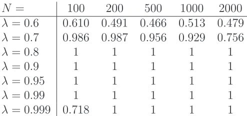
λ= 0.6 0.610 0.491 0.466 0.513 0.479

λ= 0.7 0.986 0.987 0.956 0.929 0.756

λ= 0.8 1 1 1 1 1

λ= 0.9 1 1 1 1 1

λ= 0.95 1 1 1 1 1

λ= 0.99 1 1 1 1 1

λ= 0.999 0.718 1 1 1 1

Table 2: PRDRG networks: frequency with which the likelihood ratio correctly predicted that the network is periodic rather than linear.

a fixed N. This is consistent with the fact that decreasing the sparsity provides more information to the algorithm; the same argument accounts for the slightly improved performance on periodic networks in Table 2 over linear in Table 1. Of course, at the extreme case of λ = 1 all graphs are completely full and hence there can be no meaningful distinction, which explains the poor performance for

λ= 0.999 and small N.

Overall, Tables 1 and 2 give us some confidence that the biological data sets to be studied in the next section are amenable to analysis.

5

Biological Data Sets

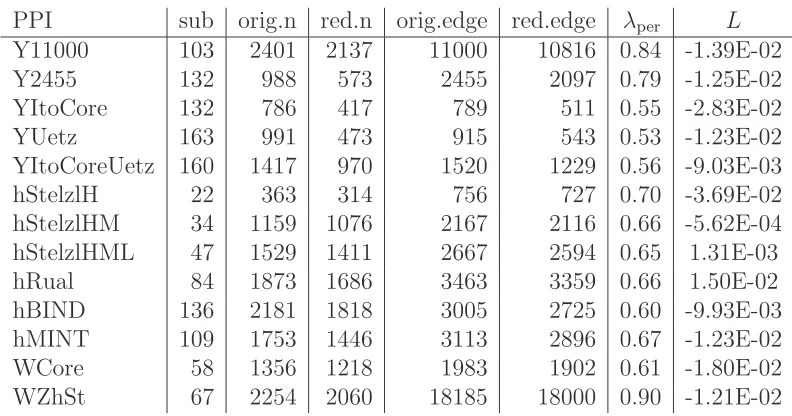
PPI sub orig.n red.n orig.edge red.edge λper L

Y11000 103 2401 2137 11000 10816 0.84 -1.39E-02

Y2455 132 988 573 2455 2097 0.79 -1.25E-02

YItoCore 132 786 417 789 511 0.55 -2.83E-02

YUetz 163 991 473 915 543 0.53 -1.23E-02

YItoCoreUetz 160 1417 970 1520 1229 0.56 -9.03E-03

hStelzlH 22 363 314 756 727 0.70 -3.69E-02

hStelzlHM 34 1159 1076 2167 2116 0.66 -5.62E-04

hStelzlHML 47 1529 1411 2667 2594 0.65 1.31E-03

hRual 84 1873 1686 3463 3359 0.66 1.50E-02

hBIND 136 2181 1818 3005 2725 0.60 -9.93E-03

hMINT 109 1753 1446 3113 2896 0.67 -1.23E-02

WCore 58 1356 1218 1983 1902 0.61 -1.80E-02

WZhSt 67 2254 2060 18185 18000 0.90 -1.21E-02

Table 3: Linear versus period reordering for protein-protein interaction data sets.

real world networks and, consequently, close and long-distance neighbours can be better differentiated with the new algorithm.

We analyzed thirteen PPI networks of three different eukaryotic organisms: yeast, worm and human. Two yeast PPI networks are described in [31]: a network defined by the top 11000 interactions (denoted Y11000 in Table 3) and its high confidence part (Y2455). Here, an increase in confidence corresponds to keeping only those links that are consistent with other sources of biological data, so higher confidence networks have fewer edges and should contain fewer false positives. A further three yeast PPI networks are the “core” from [16], the network from [29] and the union of both, denoted YItoCore, YUetz and YItoCoreUetz, respectively. Human PPI networks used in our experiments include three networks of dif-ferent confidence level: high (hStelzlH), high and medium (hStelzlHM) and high, medium and low (hStelzlHML) from [26] and a network from [21] (hRual). A further two networks were downloaded from databases BIND and MINT [3, 33] (hBIND and hMINT). Finally, two worm PPI networks were tested: WCore de-notes the worm C. elegans “core” PPI network [18] and WZhSt dede-notes the worm PPI network from [34].

Note that PPI networks generally consist of a set of disconnected components orsubnetworks. It is known that if a network hask subnetworks then the lowest

0 1000 2000 0

500

1000

1500

2000

Original Data

0 1000 2000 0

500

1000

1500

2000

Linear

0 1000 2000 0

500

1000

1500

2000

Periodic

Figure 3: Y11000 - PPI network from [31]: 2137 proteins and 10816 interactions: original adjacency matrix, the linear and periodic reorderings. The network is classifed as periodic (L=₋1.39E₋02<0).

ratio L.

We see from Table 3 that eleven out of the thirteen networks studied, including the high and high-medium confidence networks, have a negative likelihood ratio, indicating periodicity. Further, the values of the ratio are comparable with those arising when we tested data generated from the pRDRG and RDRG models.

To back up these results we now show some qualitative pictures. The Yeast PPI network Y11000 consists of 11000 interactions between 2401 proteins. There are 103 subnetworks and the largest component involves 2137 proteins and 10816 interactions. Note that by reducing the original network to its largest subnetwork we removed only 264 proteins (11%) and 184 edges (1.7%). Figure 3 shows the adjacency matrices for linear and periodic spectral reorderings of these 2137 proteins. We see that the periodic reordering places interactions (edges) into the off-diagonal corners, thereby reducing the envelope around the diagonal, relative to the linear version. This supports the negative likelihood ratio ofL=₋1.39E₋

02.

Figure 4 shows linear and periodic reorderings of YItoCore. The largest com-ponent consists of 417 proteins (out of 786) and 511 interactions (reduced from 789). This network is very sparse, with less than two edges per node on average. We obtained narrow envelopes with both reorderings; but in the periodic case the interactions are more tightly arranged along the diagonal, and this is reflected in the negative valueL=₋2.83E₋02.

0 200 400 0

100

200

300

400

Original Data

0 200 400

0

100

200

300

400

Linear

0 200 400

0

100

200

300

400

Periodic

Figure 4: YItoCore - PPI network from [16]: 417 proteins and 511 interactions. The network is classified as periodic (L=₋2.83E₋02<0).

0 500 1000 0

500

1000

Original Data

0 500 1000 0

500

1000

Linear

0 500 1000 0

500

1000

Periodic

Figure 5: hStelzlHML - PPI network from [26]: 1411 proteins and 2594 interac-tions. The network is classified as linear (L= 1.31E₋03>0).

classified as periodic L=₋3.69E₋02<0 rather than linear; see Figure 6.

6

Summary

0 100 200 300 0

100

200

300

Original Data

0 100 200 300 0

100

200

300

Linear

0 100 200 300 0

100

200

300

Periodic

Figure 6: hStelzlH - PPI network from [26]: 314 proteins and 727 interactions. The network is classifed as periodic (L=₋3.69E₋02<0).

AcknowledgementThis manuscript is dedicated to the memory of the late Ron Mitchell. PG and DJH remember him with great fondness as a wonderfully warm and inspirational colleague.

References

[1] U. Alon,An Introduction to Systems Biology, Chapman & Hall/CRC,

Lon-don, 2006.

[2] C. J. Alpert and S.-Z. Yao, Spectral partitioning: The more

eigenvec-tors, the better, Proceedings of the 32nd Conference on Design Automation, (1995), pp. 195–200.

[3] G. D. Bader, D. Betel, and C. W. V. Hogue,BIND: the biomolecular

interaction network database, Nucleic Acids Research, 31 (2003), pp. 248– 250.

[4] S. T. Barnard, A. Pothen, and H. D. Simon, A spectral algorithm

for envelope reduction of sparse matrices, Numerical Linear Algebra with Applications, 2 (1995), pp. 317–334.

[5] C. H. Q. Ding, X. He, H. Zha, M. Gu, and H. D. Simon,A min-max

cut algorithm for graph partitioning and data clustering, in Proceedings of the 1st IEEE Conference on Data Mining, 2001, pp. 107–114.

[6] I. S. Duff, A. M. Erisman, and J. K. Reid,Direct Methods for Sparse

Matrices, Oxford University Press, 1986.

[7] L. Eld´en,Matrix Methods in Data Mining and Pattern Recognition, SIAM,

[8] P. Erd¨os and A. R´enyi, On random graphs, Publ. Math. Debrecen, 6 (1959), pp. 290–297.

[9] E. N. Gilbert,Random graphs, Ann. Math. Statist., 30 (1959), pp. 1141–

1144.

[10] P. Grindrod, Range-dependent random graphs and their application to

modeling large small-world proteome datasets, Physical Review E, 66 (2002), pp. 066702–1 to 7.

[11] P. Grindrod, D. J. Higham, and G. Kalna, Perodic reordering,

06/2008, University of Strathclyde Mathematics Research Report, 2008.

[12] D. J. Higham, Unravelling small world networks, J. Comp. Appl. Math.,

158 (2003), pp. 61–74.

[13] , Spectral reordering of a range-dependent weighted random graph, IMA J. Numer. Anal., 25 (2005), pp. 443–457.

[14] D. J. Higham, G. Kalna, and M. Kibble, Spectral clustering and its

use in bioinformatics, J. Computational and Applied Math., 204 (2007), pp. 25–37.

[15] Y. Hu and J. A. Scott, HSL_MC73: A fast multilevel Fiedler and

pro-file reduction code, RAL-TR-2003-36, Numerical Analysis Group, Computa-tional Science and Engineering Department, Rutherford Appleton Labora-tory, 2003.

[16] T. Ito, K. Tashiro, S. Muta, R. Ozawa, T. Chiba, M. Nishizawa,

K. Yamamoto, S. Kuhara, and Y. Sakaki, Toward a protein-protein

interaction map of the budding yeast: A comprehensive system to examine two-hybrid interactions in all possible combinations between the yeast pro-teins, PNAS, 97 (2000), pp. 1143–1147.

[17] G. Kalna, J. K. Vass, and D. J. Higham,Multidimensional partitioning

and bi-partitioning: analysis and application to gene expression datasets, International Journal of Computer Mathematics, 85 (2008), pp. 475–485.

[18] S. Li, C. M. Armstrong, N. Bertin, H. Ge, S. Milstein, M. Boxem,

S. van den Heuvel, F. Piano, J. Vandenhaute, C. Sardet, M. Ger-stein, L. Doucette-Stamm, K. C. Gunsalus, J. W. Harper, M. E.

Cusick, F. P. Roth, D. E. Hill, and M. Vidal,A map of the

interac-tome network of the metazoan C. elegans, Science, 303 (2004), pp. 540–543.

[19] M. E. J. Newman,The structure and function of complex networks, SIAM

Review, 45 (2003), pp. 167–256.

[20] M. E. J. Newman, C. Moore, and D. J. Watts,Mean-field solution of

the small-world network model, Physical Review Letters, 84 (2000), pp. 3201– 3204.

[21] J. F. Rual, K. Venkatesan, T. Hao, T. Hirozane-Kishikawa,

A. Dricot, N. Li, G. F. Berriz, F. D.Gibbons, M. Dreze, N. Ayivi-Guedehoussou, N. Klitgord, C. Simon, M. Boxem, S. Milstein, J. Rosenberg, D. S. Goldberg, L. V. Zhang, S. L. Wong, G. Franklin, S. Li, J. S. Albala, J. Lim, C. Fraughton, E. Llam-osas, S. Cevik, C. Bex, P. Lamesch, R. S.Sikorski, J. Van-denhaute, H. Y. Zoghbi, A. Smolyar, S. Bosak, R. Sequerra, L. Doucette-Stamm, M. E. Cusick, D. E. Hill, F. P. Roth, and

M. Vidal,Towards a proteome-scale map of the human proteprotein

in-teraction network, Nature, 437 (2005), pp. 1173–1178.

[22] J. Shi and J. Malik, Normalized cuts and image segmentation, IEEE

Transactions on Pattern Analysis and Machine Intelligence, 22 (2000), pp. 888–905.

[23] D. S. Sivia,Data Analysis: A Bayesian Tutorial, Oxford University Press,

second ed., 2006.

[24] D. Skillicorn,Understanding Complex Datasets: Data Mining using

Ma-trix Decompositions, CRC Press, 2007.

[25] A. Spence, Z. Stoyanov, and J. K. Vass, The sensitivity of spectral

clustering applied to gene expression data, in Proceedings of the 1st Inter-national Conference on Bioinformatics and Biomedical Engineering, 2007, pp. 1343–1346.

[26] U. Stelzl, U. Worm, M. Lalowski, C. Haenig, F. H.

Brem-beck, H. Goehler, M. Stroedicke, M. Zenkner, A. Schoen-herr, S. Koeppen, J. Timm, S. Mintzlaff, C. Abraham, N. Bock, S. Kietzmann, A. Goedde, E. Toksz, A. Droege, S. Krobitsch,

B. Korn, W. Birchmeier, H. Lehrach, and E. E. Wanker,A human

[27] G. Strang,Computational Science and Engineering, Wellesley-Cambridge Press, 2008.

[28] S. H. Strogatz,Exploring complex networks, Nature, 410 (2001), pp. 268–

276.

[29] P. Uetz, L. Giot, G. Cagney, T. A. Mansfield, R. S. Judson, J. R.

Knight, E. Lockshon, V. Narayan, M. Srinivasan, P. Pochart, A. Qureshi-Emili, Y. Li, B. Godwin, D. Conover, T. Kalbfleish, G. Vijayadamodar, M. Yang, M. Johnston, S. Fields, and J. M.

Rothberg,A comprehensive analysis of protein-protein interactions in

sac-charomyces cerevisiae, Nature, 403 (2000), pp. 623–627.

[30] R. Van Driessche and D. Roose, An improved spectral bisection

algo-rithm and its application to dynamic load balancing, Parallel Computing, 21 (1995), pp. 29–48.

[31] C. von Mering, R. Krause, B. Snel, M. Cornell, S. G. Oliver,

S. Fields, and P. Bork, Comparative assessment of large-scale data sets

of protein-protein interactions, Nature, 417 (2002), pp. 399–403.

[32] D. J. Watts and S. H. Strogatz, Collective dynamics of ‘small-world’

networks, Nature, 393 (1998), pp. 440–442.

[33] A. Zanzoni, L. Montecchi-Palazzi, M. Quondam, G. Ausiello,

M. Helmer-Citterich, and G. Cesareni,MINT: a molecular

interac-tion database, FEBS Letters, 513 (2002), pp. 135–140.

[34] W. Zhong and P. W. Sternberg,Genome-wide prediction of C. elegans