Rochester Institute of Technology
RIT Scholar Works
Theses Thesis/Dissertation Collections
2011
An Integrated environment for data acquisition
with dynamic changes in wireless sensor networks
Albert Nurgaliev
Follow this and additional works at:http://scholarworks.rit.edu/theses
This Thesis is brought to you for free and open access by the Thesis/Dissertation Collections at RIT Scholar Works. It has been accepted for inclusion in Theses by an authorized administrator of RIT Scholar Works. For more information, please [email protected].
Recommended Citation
An Integrated Environment for Data Acquisition with Dynamic Changes
in Wireless Sensor Networks
Albert Nurgaliev
M. S. Computer Science Thesis
Department of Computer Science
Rochester Institute of Technology
Rochester, New York
Submitted in partial fulfillment of the requirements of a
Master of Science Degree in Computer Science
COMMITTEE
________________________________________________________________________
CHAIR: Professor Leon Reznik DATE
________________________________________________________________________
READER: Associate Professor Minseok Kwon DATE
________________________________________________________________________
OBSERVER: Professor Hans-Peter Bischof DATE
2
Abstract
The wireless sensor network (WSN) is an important technology with a wide variety of
diverse applications in such domains as healthcare, military forces and environmental
monitoring.
Our research aims at developing methods and tools capable of addressing WSN
problems such as energy constraint, low memory, and computation capability of a sensor node
by implementing a new WSN design concept, improving existing and developing new
protocols. Our research goal is to develop novel generic methodologies supporting a higher
level of design flexibility and possible architectural optimization against multiple criteria such
as the quality of data (QoD), quality of service (QoS), and lifetime extension. Application
requirements may vary in terms of abovementioned parameters and consequently there is no
single platform that can be applied to all domains. Moreover, current methods do not provide
opportunities for dynamic changes of either protocols or their parameters, which might
improve WSN agility and survivability in a harsh environment. This problem can be solved
by integrating various protocols at different layers within a single framework and supporting
their dynamic selection in order to adapt the network to varying application requirements.
This thesis develops a mechanism which facilitates structural design and
implementation of an Integrated Environment for Data Acquisition with Dynamic Changes
(IEDADC). It features adaptation and integration of protocols, protocol switching and
automatic or manual selection as well as the implementation of quality assurance and
localization techniques.
The design methodology is tested by implementing a SN prototype consisting of a
base station and sensor nodes. Sun Small Programmable Object Technology is used as a
hardware basis for this work. The software has been developed in Java programming
language including the host and sensor nodes’ applications.
The conducted experiments have confirmed the higher level of design flexibility and
3
Table of Contents
LIST OF FIGURES ... 4
1. INTRODUCTION ... 7
2. BACKGROUND ... 10
3. RELATED WORK ... 15
3.1LOCALIZATION METHODOLOGIES ... 15
3.2A FRAMEWORK DESIGNING METHODOLOGIES ... 16
3.3QOS OPTIMIZATION METHODOLOGIES ... 19
3.4QOD OPTIMIZATION METHODOLOGIES ... 21
4. HYPOTHESIS ... 23
5. DESIGN ARCHITECTURE AND IMPLEMENTATION ... 24
5.1 THE FRAMEWORK ARCHITECTURE ... 25
5.1.1 View ... 25
5.1.2 Model ... 34
5.1.3 Plug-in ... 37
5.1.4 Proxy ... 38
5.2 THE FRAMEWORK IMPLEMENTATION ... 39
6. EXPERIMENTS AND RESULTS ... 45
6.1INVESTIGATION OF THE LOCALIZATION ALGORITHM ACCURACY ... 45
6.2INVESTIGATION OF THE QA MECHANISMS’ OPERATION ... 54
6.3INVESTIGATION OF THE CROSS-LAYER INTEGRATION OF PROTOCOLS ... 56
7. CONCLUSION. MAIN RESEARCH RESULTS ... 69
4
List of figures
Figure 1.1 - An example of a Wireless Sensor Network ... 7
Figure 1.2 - A wireless sensor node’s architecture ... 7
Figure 1.3 - The relationship between the network lifetime and the accuracy of data in a WSN ... 9
Figure 2.1 - Schematic representation of a WSN working under the PEAS protocol ... 11
Figure 2.2 - Wake-up intervals for deterministic sleeping time ... 12
Figure 2.3 – Spreading the wake-up periods throughout the time ... 12
Figure 2.4 - Schematic overview of a network with the degree of coverage set to two ... 13
Figure 2.5.1 - Schematic overview of a WSN, with a low probing range ... 14
Figure 2.5.2 - Schematic overview of a WSN, with a high probing range ... 14
Figure 3.1 - System architecture for habitat monitoring [5]. ... 18
Figure 3.2 - An example of a single-source multiple-path WSN ... 20
Figure 3.3 - An example of a multiple-source single-path WSN ... 20
Figure 3.4 - ESRT operation overview. ... 21
Figure 3.5 - Cluster-based WSN architecture [2] ... 22
Figure 5.1 - The framework architecture... 25
Figure 5.2 - The “Protocol information” tab of the framework ... 27
Figure 5.3 - The “Signal strength” tab of the framework. ... 28
Figure 5.4 - The “Data” tab of the framework. ... 29
Figure 5.5 - The “Clusters” tab of the framework. ... 30
Figure 5.6.1 - Graph view of the network ... 31
Figure 5.6.2 - A graph of an average energy use measured in mA (y-axis) over time measured in minutes (x-axis) ... 31
Figure 5.7 - The “Signals” tab of the framework. ... 32
Figure 5.8 - The “Settings” tab of the framework. ... 32
Figure 5.9 - The references between modules of the IEDADC. ... 35
Figure 5.10 - IEDADC sensor network interaction overview. ... 37
5
6
7
1.
Introduction
A typical wireless sensor network (WSN) is composed from two kinds of nodes [3]
(fig. 1.1). The first is the full-function device (FFD), which serves as a coordinator of the
network. An example to FFD can be a base station, it can also be called a sink node. The
second kind is the reduced-function device (RFD), a simple device with little resource
requirements and computational capabilities. A sensor node is an RFD which is also called a
[image:8.612.135.474.212.436.2]mote.
Fig. 1.1.An example of a Wireless Sensor Network1.
There are four main components in a sensor node: a sensing unit, a processing unit, a
communication unit, and power supply [20] [22] (fig. 1.2).
Fig. 1.2. A wireless sensor node’s architecture2.
1
The figure is taken from [7]. 2 The figure is taken from [2].
3
See the JUNG2 2.0 API at http://jung.sourceforge.net/doc/api/index.html for details.
4 The picture is taken from http://blogs.sun.com/roger/entry/location_location_location_radio
5
8
A sensing unit can be composed of several sensors, which monitor various
environmental characteristics such as temperature, humidity, pressure or light. The processing
unit includes a small storage in a form of flash memory. It is responsible for performing tasks,
processing data and controlling certain functionalities of a sensor node. A communication unit
is represented by a transceiver, which provides receiving and transmitting of data and wireless
communication between nodes. The main power supply for a sensor node is a battery. The
energy constraint is the main problem related to efficient application of a WSN. While energy
is consumed for sensing, data processing and communication, the former task consumes the
majority of energy recourses [20] [22].
Our research aims at developing methods and tools capable of addressing typical WSN
problems such as energy constraint, low memory and computation capability of a sensor node
by implementing a new WSN design concept, as well as improving existing and developing
new protocols. Our research goal is to develop novel generic methodologies supporting a
higher level of design flexibility and possible architectural optimization against multiple
criteria such as the quality of data (QoD), quality of service (QoS), and lifetime extension.
Application requirements may vary in terms of abovementioned parameters and consequently
there is no single platform that can be applied to all domains. Moreover, current methods do
not provide opportunities for dynamic changes of either protocols or their parameters, which
might improve WSN agility and survivability in a harsh environment. Therefore this problem
can be solved by integrating various protocols at different layers within a single framework
and supporting their dynamic selection in order to adapt the network to varying application
requirements.
Although many efficient protocols have been proposed for WSNs [9-11] [21-22] there
is still an open research problem related to cross-layer optimization. Optimizing and analyzing
protocols can improve system performance and determine their benefits and limitations, but
WSN can also benefit from cross-layered approach. For example, depending on the
application, a higher degree of coverage may be required to increase the accuracy of the
sensed data. However, the sensor network lifetime depends on the number of active nodes and
connectivity of the network, so energy must be used efficiently in order to maximize the
9
network lifetime (fig. 1.3). In this case, providing an application layer service on top of the
protocol stack can efficiently resolve the problem of network lifetime extension.
This research mainly concentrates on development and implementation of a design
methodology which determines, regulates and possibly optimizes the following parameters:
network lifetime, cross-layer integration, QoS, data aggregation and localization.
a) High accuracy of sensed
data, low network lifetime.
b) Long network lifetime, low
accuracy of data.
c) An example of a balance
between the network lifetime
and the accuracy of data.
Fig. 1.3. The relationship between the network lifetime and the accuracy of data in a WSN (w – working node,
s – sleeping node).
Developing an efficiently operating platform for WSNs is an important task. Agility
mechanisms must be incorporated in such a way that they are transparent to users and must
introduce minimal functional and performance impacts. These techniques must be employed
in combination with a system-level architecture that links these mechanisms together, to
ensure optimal effectiveness and proper management.
This thesis develops a mechanism which facilitates structural design and
implementation of an Integrated Environment for Data Acquisition with Dynamic Changes
(IEDADC). It features adaptation and integration of protocols, protocol switching and
selection either automatically or manually as well as some other features such as
implementation of quality assurance and localization techniques.
The design methodology is tested by implementing a SN prototype consisting of a
base station and sensor nodes. Sun SPOT (Small Programmable Object Technology) is used
as a hardware basis for this work. The software has been developed in Java programming
10
The organization of this paper is as following. Section 2 provides the analysis of the
protocols used in this work. Section 3 discusses the related work. Section 4 states the
hypothesis for the thesis. Section 5 introduces the design architecture and discusses the
implementation of the optimization techniques used in this work. Section 6 presents the
experiments performed using IEDADC and their results. Section 7 describes the results of this
research and gives conclusion for this work.
2.
Background
According to the TCP/IP model of network architecture there are five layers:
Application Transport Network Data Link Physical
A WSN also borrows this network architecture [22]. However, the sensor network
constraints mentioned previously pushed the researchers to develop more energy efficient
standards and protocols than the popular ad-hoc protocols. These standards take into account
low computational capabilities of sensor nodes, the number of elements present in the
network, which is relatively higher than in ad-hoc networks, and their limited power supply.
As a result of these efforts the IEEE 802.15.4-2006 standard has been developed. This
standard specifies the physical and MAC layers for low rate WPANs, with the main emphasis
made on low-cost, low-speed communication between devices [3]. The standard does not
define higher level layers, so additional specifications exist offering protocols on the higher
layers. These protocols / standards provide additional integral solutions, such as quality of
service, quality of data and topology control. Examples of such additional standards are
ZigBee alliance [24], TinyOS [17] and others. Sun SPOT is not a member of ZigBee alliance,
and IEEE 802.15.4 is the only standard implemented in this technology. This allows
development of a network stack on top of the IEEE 802.15.4 standard. Development of
numerous protocols [7] [9-10] [22] demonstrates the fact that there exist many application
requirements for WSNs. Therefore integrating various protocols at different layers within a
single framework and supporting their dynamic selection would allow for adapting the
11
In order to address the issue of extending the network lifetime in a harsh working
environment, the implementation of PEAS (Probing Environment and Adaptive Sleeping)
[21] protocol is presented in this work. Customization of its parameters affects the network
lifetime, network connectivity and the QoD. Two other protocols are provided as the part of
the radio communication library of the Sun SPOT SDK. This work employs all three
protocols to develop methods for dynamic switching of protocols or altering their network
parameters to fit varying application requirements.
Each node in PEAS protocol can be in three different states: sleeping, probing and
active. All nodes initially start with the sleeping state, from which they periodically enter a
probing state. During this state the sensor will determine whether to activate and provide a
coverage of sensing area or go back to sleep (Fig. 2.1).
Fig. 2.1. Schematic representation of a WSN working under the PEAS protocol; w – working sensor, s –
sleeping sensors, p – probing sensor, r – sensing range of a working sensor.
Probing time needs to be tuned carefully to preserve a balance between energy saving
and robustness. If it is too long, a node failure would be unnoticed for a long time, on the
other hand a probing period that is too short may result in wasted power. Also in this protocol,
the wake-up intervals are spread over time for two particular reasons: preventing extended
sensor outage, and avoiding collisions. For example, if a node fails, the sensing area might be
uncovered for a long time, so a wake-up interval is needed to detect the outage. In case of
many sensor nodes waking up at the same time, collisions can be mitigated by properly
setting the wake-up intervals. The following figures show the wake-up intervals when using
deterministic sleeping time (Fig. 2.2) and wake up intervals, which are spread over time (Fig.
12 Fig. 2.2. Wake-up intervals for deterministic sleeping time. Long gaps between two wake-ups, a lot of sensors
wake-up at the same time.
Fig. 2.3. Spreading wake-up times throughout the time. Short gaps between two wake-ups and no collisions
happen when one sensors wakes-up.
Moreover, the PEAS protocol dynamically adjusts the sleeping time, so that node
failures do not affect the overall spread of waking times. This protocol has been modified to
support dynamic customization of the following parameters: the number of working nodes,
the sleeping time duration and the probing range. Setting up the parameters of this protocol
can influence the overall operation of the network.
The number of working sensors (fig. 2.4) parameter directly affects the network
lifetime duration and the quality of data (QoD) for a certain region. Setting this parameter to
one would maximize the network lifetime, minimizing the accuracy of the received data.
Increasing the number of working sensors would lower the network lifetime, on the other
13 Fig. 2.4. Schematic overview of a network with the degree of coverage set to two; where w – working sensor; s
– sleeping sensor; p – probing sensor; Rp – probing range.
The second parameter, the sleeping time duration, affects the frequency at which
probing is performed by a sensor node. This influences both working and sleeping nodes’
battery discharge levels and how fast the node failures are determined. The battery discharge
level is affected when a probing node sends a probing message and waits for a reply from a
working node(s) for a certain amount of time, while the working node spends its energy by
receiving the probing message and sending back the reply. So the higher the frequency of
entering the probing state, the higher is the energy overhead from using the PEAS protocol.
On the other hand, setting the sleeping time duration higher would result in longer periods
when a failure of a working sensor node would stay unnoticed. Balancing between the energy
overhead and node failure notification is application specific and setting the sleeping time
duration parameter should be considered individually for every case.
The last parameter, the probing range, affects the number of sensors that will enter the
working state in the network. This is not to confuse with the first parameter, which determines
the number of working sensors per one area. The probing range parameter determines the
number of such areas and their size. In the implementation of the protocol we used a threshold
filtering rule regarding the received signal strength [21] as a probing range parameter. This
implies that a sensor will react to a message only if its signal strength of a message is greater
14 Fig. 2.5.1. Schematic overview of a WSN, with a low
probing range. It results in entering the probing node
p to the working state. Rp – probing range; Rt –
transmission range; w – working sensor node; s –
sleeping sensor node; p – probing sensor node.
Fig. 2.5.2. Schematic overview of a WSN, with a
high probing range. It results in having more sleeping
nodes around the working node. Rp – probing range;
Rt – transmission range; w – working sensor node; s –
sleeping sensor node; p – probing sensor node.
The second protocol is called Radiogram. It is a part of a Sun SPOT SDK radio
communication library. It provides datagram based communication between devices and there
are no guarantees that the datagram will be delivered; also datagrams can be delivered out of
order or delivered more than once [13]. As a result of this, the Radiogram protocol is
unreliable. The protocol supports several modes: client-server, broadcast and point-to-point.
When opening the client-server connection, the server side can receive any radiograms sent
on a given port whether they are broadcast packets or packets sent specifically to this sensor.
Broadcast mode delivers radiograms to all listeners with no delivery guarantees.
Point-to-point mode creates connection between two peers only. Along with the payload every
radiogram automatically carries, from one node to another, such information as the signal
strength (measured in dB), the link quality (in %), the timestamp, etc.
The third is the Radiostream protocol, which provides a socket-like peer-to-peer radio
protocol with reliable, buffered stream-based IO between two devices [13]. A connection
using this protocol is reliable, since the delivery of packets is confirmed by sending ACKs
back to the source. Every packet also carries some additional information about the
[image:15.612.78.545.52.372.2]15
3.
Related Work
This section discusses the existing methodologies proposed to address the issues of sensor nodes’ localization, a framework design development, the QoS and the QoD optimizations.
3.1 Localization methodologies
Location awareness is an open research problem in a WSN. Precise location
information may be unavailable due to the energy constraints peculiar to sensor nodes. The
use of GPS for sensor localization is extremely energy-consuming, which makes it impractical
for installation on sensor nodes. However the knowledge of sensor nodes’ location can be
very useful in such applications as tracking an object, route discovery and avoiding sensing
coverage overlap [18]. A direction-based localization scheme (DLS) [18] determines a
direction of a sensor node relative to the sink node. The main idea of DLS is the spatial
locality property, which allows sensor nodes to determine their directions according to the
packets received. The direction of a node is represented in a form of a gray code.
In localization techniques the nodes whose location is initially known are called
anchors. Messages sent by anchors are used by other nodes in the network to calculate their
relative direction. Different strategies are used in [18] to improve estimated correctness of the
localization. Overall, the results of the simulations presented in [18] demonstrate the accuracy
of DLS at around 85%.
In the current work, a localization algorithm is also introduced as a part of the QA
mechanism of the framework. This algorithm calculates the approximate signal strength level
between two sensor nodes. A helper SPOT is referred to as an anchor in this work. The
selection of a helper SPOT is done during the localization process, while anchors in [18] are
selected statically and their location is known in advance. The main idea of our localization
algorithm is the capability to measure an approximate signal strength value between two
nodes by means of triangulation.
Section 5.2 describes the details of our localization algorithm; meanwhile experiment
results demonstrating the correctness of the algorithm and nodes’ signal strength distribution
16 3.2 A framework designing methodologies
The application developed in [6] analyzes the number of neural network (NN)
architectures and signal waveforms to detect novelties in a radio transmission coming from
wireless sensors. In order to increase chances to detect novelties in signals, the application has
different parameters to configure in its GUI, such as NN architecture, its learning rate, novelty
distance, threshold, etc. The application includes twenty-six NN architectures, which a user
can select from the GUI. Based on the choice of NN and its settings, the application detects
novelties in the signal and notifies the user though email or alarm sound. In order to determine
which NN architecture returns the least error with the signal, the user has to manually test the
performance of each NN on the same signal and compare the results. However, the novel
contribution done in this work is the ability to simulate signals, as well as to experiment with
NN (either custom made or already implemented in MATLAB). Interaction with the program
is done through a user-friendly GUI. This contribution opens new ways for developing and
testing NN, serving as a testing field for new NN architectures. The approaches used in
developing the application’s front-end in [6] were used as the basis for the development of the IEDADC’s GUI.
The work in [16] introduces the prototype framework for automated data quality
assessment. In order to understand the problems related to QA consider a situation when three
sensors are measuring the temperature in a room. Apparently, when one of the sensors starts
sending different temperature information than the other two sensors, it seems suspicious,
because the temperature in a room is most likely to stay constant over the area of the room.
QA mechanisms do not try to determine the reasons which stand behind such misbehavior.
Instead the data is assigned a green, a yellow or a red flag. The color of a flag has a certain
meaning: the green flag is a good data, the red flag is a bad data and the yellow flag is the
quality in-between. It is important to note that the red flag does not necessarily mean that the
data is wrong, but instead it indicates that this data and the area from which it was sensed
requires an immediate attention. These approaches are taken as a basis for the development of
the QA aspects in IEDADC.
An Interactive and Extensible Framework for Execution and Monitoring of Wireless
Sensor Networks [4] adds extra distributed services on top of Directed Diffusion protocol to
17
on Directed Diffusion, the framework is extensible to be used by any other network protocol
and distributed services related to the protocol.
The framework in [4] is written in C++ versus Java used in current work. Also, in [4]
Sensoria WinNG sensor devices are used in the research versus Sun SPOTs in the current
work. The current work also focuses on optimization of multiple criteria, while the framework
in [4] puts the emphasis on the network protocol performance only, i.e. average network
traffic per node. In addition, the current work investigates the ways to automate some
processes in the framework, based on the data incoming from the sensor nodes. This would
provide a certain level of intelligence to the system, aiming to reduce the workload from a
user.
Another framework presented in [1] introduces the design and implementation of
MAPS (Mobile Agent Platform for Sun SPOT). It is also a Java-based framework for wireless
sensor networks based on Sun SPOT technology, like the framework presented in the current
work. The authors of the paper utilize an agent-oriented programming paradigm on WSN
applications. Novel contributions of this paper to the WSN programming research area are:
Introducing a platform that allows an effective Java-based development of agent-based
applications;
Investigation of the Sun SPOT technology for supporting mobile agent-based
applications and systems.
The introduced paradigm has already shown its effectiveness and efficiency in
IP-based highly dynamic distributed environments [1], hence the authors of the paper integrate
these paradigms into the MAPS framework to achieve same results in WSN applications.
The experiments in the healthcare domain, which involved real-time monitoring of
human activities, demonstrated the effectiveness and the suitability of the agent-based
approach to program WSN applications. However, the MAPS performance benchmarking
demonstrated that the serialization and transportation of agents are very time and energy
consuming operations [1].
IEDADC intends to harness effectiveness and efficiency of WSN application through
dynamic selection and customization of the protocol parameters, compared to the
18
In [5] authors of the paper incorporate the concept of supply chain into a WSN. They
propose a hybrid data dissemination framework based on the supply chain (SC) methodology.
According to the proposed methodology, a supply chain is a series of links between suppliers
and consumers, which involve such activities as the acquisition of raw materials,
manufacturing, and delivery of produced goods to the end consumers [5].
This concept has been projected to a WSN model. As a result the network is
partitioned into functional regions, each responsible for a certain task reflecting the SC
methodology (fig. 3.1). The authors of the paper use a habitat monitoring example to illustrate
their scheme.
Fig. 3.1. System architecture for habitat monitoring [5].
Nodes in each area are responsible for different tasks. Sensor nodes in a manufacturing
area, for example, are responsible for data acquisition and aggregation. Transportation area is
responsible for delivery of data to the sink nodes. Warehouse area is responsible for providing
a temporary storage of data until it has been requested by a sink node. Service area is where
the sink nodes are located.
This kind of diversification of nodes’ tasks provides such features as flexibility and
scalability of WSN applications as well as improved reliability and energy efficiency of the
network.
The framework developed in [5] uses various routing protocols to different regions in
order to provide better performance in terms of reliability and efficient energy usage. This
contrasts with the current work, which uses a single protocol for the entire network. However,
19
customization of its parameters. Both of the frameworks are designed to have the ability to
extend their functionality by adding other WSN protocols. This feature provides the
scalability of a framework and improves its flexibility for various applications.
Implementation of the SC methodology requires deployment of a comparatively large
number of sensors to maintain functionality of the areas introduced in [5]. Therefore SC
methodology is not applicable in a sparsely deployed network or a network with a small
number of sensor nodes.
3.3 QoS optimization methodologies
The discussion below will define the QoS model used in this work as well as provide
alternative approaches in defining a QoS model. Despite the fact that this parameter is always
application specific, it is usually defined by the following categories: reliability, timeliness
and throughput [19] [23]. Reliability implies certain level of a guarantee to deliver data from
source to destination. The higher the guarantee to deliver data, the more reliable the protocol
is. In terms of protocols, sending acknowledgements for each received packet is a way to
make the protocol reliable. Radiostream is an example of a reliable protocol for WSN. The
second parameter is a timeliness of a data delivery, which means the data should be delivered
within a certain time limit. The throughput is specified as a bandwidth. It is the effective
number of data, transported within a certain period of time [19]. If all of these parameters are
satisfied then in this work we can state that the protocol provides a high QoS.
In order to achieve a high QoS it is always necessary to add some redundancy to the
protocol. Therefore minimizing energy consumption and maximizing QoS are two typically
conflicting requirements [19]. Indeed, acknowledgements (ACKs) used by Radiostream
protocol make it reliable. However, sending ACKs consumes energy, which is vital for
sensors. In general, addition of any kind of redundancy increases the sensors’ workload
resulting in increasing the QoS and trading-off the network lifetime. The problem of keeping
both of these parameters at a high level becomes one of the major problems investigated in
WSN. For this reason multiple alternative approaches addressing this issue exist [2] [7] [9]
[12]. For example, an Adaptive Fault-tolerant QoS Control (AFTQC) algorithm [2] uses
20 Fig. 3.2. An example of a single-source multiple-path WSN.
Determining an optimal redundancy level to achieve a high QoS and long network
lifetime is one of the problems investigated by the authors of the paper. According to the
results of the simulations, it appears that the value of mpset to three is the optimal parameter.
Also they demonstrate that in comparison with the traditional “acknowledgement and
retransmission on timeout” mechanism, AFTQC algorithm performs better in terms of the
network lifetime under various number of redundant paths and sources (ms) [2] (Fig. 3.3).
Fig. 3.3. An example of a multiple-source single-path WSN. S1, S2, S3 is the first, the second and the third
sources respectively.
The algorithm used in Sun SPOT network to find a path between source and sink is
called Link Quality Routing Protocol (LQRP) [13], which is used by default and its
functioning is transparent for a user. The user can only gain some level of control in routing
by setting a routing policy for each sensor through system properties or programmatically
[13]. IEDADC uses only one path to deliver data in comparison with multiple paths used by
AFTQC. Also, our framework uses ACKs, while AFTQC uses redundant paths to guarantee
21
sending ACKs is less energy efficient according to the simulation results from [2], it provides
a basis for further developments of more complex algorithms for high QoS. Furthermore, in
this work we will show that the use of additional service, such as PEAS protocol can increase
the network lifetime, keeping the QoS on a desired level.
The protocol, called Event-to-Sink Reliable Transport (ESRT) [11], measures the QoS
level according to the number of received packets at the sink node and notifications of
congestion in the network. The network in this protocol can operate in one of five states: No
congestion, low reliability (NC,LR), The optimal operating region (OOR), No congestion,
high reliability (NC,HR), Congestion, high reliability (C,HR), Congestion, low reliability
(C,LR). The idea here is that the sink node tries to control the sensors' reporting rate so that
the network is in the OOR. It is achieved by broadcasting a revised reporting rate to the
sensors (Fig. 3.4). The reliability is determined by the number of packets the sink node
receives, while the congestion is detected by the routing nodes, which send notifications to the
[image:22.612.201.399.339.444.2]base station.
Fig. 3.4. ESRT operation overview.
3.4 QoD optimization methodologies
Alternative approaches exist for clustering and data aggregation in WSNs [2]. Data
aggregation and clustering are mainly used to save energy by reducing the number of sensors
sending information to the sink node. It also solves the problem of QA, because
measurements from different sensors after aggregation and processing increase the accuracy
of the sensed data.
The authors of the paper [2] consider a cluster-based WSN to increase the
effectiveness of the energy use in the network. The AFTQC’s clustering algorithm creates a
cluster head (CH) which is responsible for managing the network within a cluster, i.e. send
22 Fig. 3.5. Cluster-based WSN architecture [2].
This algorithm is executed periodically to make every sensor in the cluster a CH and
therefore the workload is spread evenly among nodes.
The clustering algorithm implemented in IEDADC is provided as a part of the QA
mechanism. It is implemented on the host application (the Model module of the framework).
There are no cluster heads present in WSN and all data is sent to the base station for
processing. This approach increases the accuracy of the data. In cases when this parameter is
not prioritized, the degree of coverage can be dynamically reduced. The reason standing
behind clustering on a host application rather than keeping CH is that a CH may fail for some
reason in a harsh environment. It would result in leaving some part of the network without
coverage until another clustering is executed. In the worst case the CH can fail right away,
after the clustering. In that case the area will be uncovered for some period Tc, where Tc is the
interval between two clustering algorithm executions. In our case even if a node fails in the
network, the data is still sent by other sensor nodes in the region. In case PEAS protocol is
enabled and the working sensor fails, the sleeping time duration of every sensor is generated
in such a way that this failure shall be discovered within a short period of time and this failed
node is replaced by a new working sensor node [21].
The source redundancy refers to the use of multiple sensor nodes to report sensing
23
request, the higher the chance that data will be delivered before timeout. In this work the
source redundancy is implemented as a mechanism of QA – as more sensors send data, the
higher is the accuracy of the obtained results.
As we can see, there are multiple approaches for solving one issue. All of them may
have advantages and disadvantages compared to each other. Also the same approach can
serve as a solution for different purposes. Therefore integration of various algorithms within a
single framework would make the interaction with a WSN efficient, effective and easy to use
for many applications.
4.
Hypothesis
This work introduces the design methodology and implementation of IEDADC that
features adaptation and integration of protocols, protocol switching and automatic or manual
selection as well as other features such as an implementation of quality assurance and
localization techniques. Its GUI provides a user with such information about sensor nodes’
state as battery level, signal strength, the temperature in the region, etc. The framework
operates with Sun SPOT sensor nodes and is implemented entirely in a Java programming
language.
Based on the proposed features of the developed environment we state the hypothesis
for the thesis: The proposed design methodology of a WSN brings higher level of design
flexibility and possible optimization for multiple criteria, minimizing energy consumption
under the conditions of supporting the specified levels of QoD and QoS. QoD is assured by
the QA mechanisms employed in this framework such as clustering, data processing and
localization.
IEDADC is employed to conduct an empirical study to confirm the hypothesis.
The empirical study includes:
1) Measuring the average energy consumption of sensor nodes in the network under
various network loads with and without using the PEAS protocol;
2) Measuring the accuracy of the localization algorithm;
3) The examination of the clustering algorithm and aggregation functions’ operation.
In the following research experiments, two extreme cases are tested to evaluate the
24
using the PEAS protocol, so this service is disabled and sensors use forwarding protocol to
send their data (comparative analysis of two forwarding protocols based on their energy use is
provided). The second case, on contrary, involves only one working sensor, providing the
k-coverage parameter set to one. Also different forwarding protocols are used in combination
with the PEAS protocol to evaluate its performance (in terms of network lifetime) under
different network loads.
The results from these two experiments will demonstrate us the best and the worst
cases for energy consumption of sensor nodes in a WSN. According to these results a user can
customize the parameters of the protocol to achieve other goals, such as better QA. Further
discussion of the effects from varying each of the PEAS protocol parameters will help to
maintain the changing application demands in a WSN.
The accuracy of the localization algorithm is determined by comparing the calculated
signal strength value to the expected value in that region. The experiment involves placing
groups of sensor nodes at various distances from each other. The calculated signal strength
value is considered to be accurate if its value does not deviate from the signal strength value
of a sensor node located in the same group.
The aggregation functions’ operation is evaluated by examining the calculated
temperature values in a cluster against the real temperature values of the sensors. The
operation of the clustering algorithm is demonstrated by placing one of the sensor nodes in a
cluster into a colder environment than other nodes and observing the automatic changes made
in clustering of nodes. Section 6 describes these moments in greater details.
5.
Design architecture and implementation
Based on the problem specification, an Integrated Environment for Data Acquisition
with Dynamic Changes (IEDADC) has been developed. This framework includes two
protocols provided by Software Development Kit (SDK) and one protocol described in
section 2, as well as the implementation of a QA and localization techniques. Sun SPOT
(Small Programmable Object Technology) [15] is used as a hardware basis for this work.
25
5.1 The framework architecture
Generally, the architecture of the framework has to be simple and scalable. It must be
simple to use from the user or a developer point of view. This means that the GUI must
support simple user interactions with the WSN and human readable real-time networking
information. It must be scalable, so that new features can be added (protocols on different
network layers, plug-ins) to the framework with no or minor modification of the architecture
[4].
The architecture of the framework is composed of four modules: view, model, proxy
and plug-in. The schematic view of this architecture is shown below:
Fig. 5.1. The framework architecture.
5.1.1 View
The View module is responsible for user interaction, control and visualization of a
WSN architecture and operation. It provides the following information: the network structure
in a form of a table and a graph, where each node is a sensor and edges are the links between
sensors; the state of each sensor, such as the sensor's signal strength, the quality of data. This
module also supplies the user with more analytical, text- or table-based information about the
WSN for its further analysis.
Below is the detailed description of the front-end.
The first tab is “Protocol information” (Fig. 5.2).
On top left corner is the “Address” label, which displays the address of the base
26
have the base station start listening to the sensor nodes for connection, the user needs to press
the “Connect” button. Before connecting, it is possible to choose the protocol that will be used
from the dropdown box, next to the Connect button. Label below shows the protocol currently
in use. “Switch protocol” button allows switching current protocol used to another one
selected from the dropdown box. “Radio policy” button allows changing the policy used to control the radio antenna of sensors (see the developer’s guide for more details of how the Radio policy affects the sensors’ behavior). The Enable service button allows selecting a
distributed service from the dropdown box in order to enhance some parameters of the current
protocol. In the current implementation, this is the PEAS protocol.
The right column contains the table of currently connected sensors. First column of the
table shows the address of the sensor, the second displays the status of the sensor. The status
can be either connected or not. The third column shows the state of a sensor when running
PEAS protocol. It is either “working” or “sleeping”. As it has been mentioned, there are three
states in PEAS protocol: sleeping, probing and working, but since importance of the probing
state is not so high, this state is not displayed in the View. In terms of implementation, this
implies the sensor notifies the base station only if it is about to enter working state; if there
was no such notification, by default the state is considered as “sleeping”. It is clear when the
status of a node is “Connected”, however, some elaboration is needed regarding status “Not
connected”. When the sensor node first connects to the base station its address is displayed at
this table and will never be removed from it (only after restart of the framework). Its status
can be changed to “Not connected” when the base station losses the connection to that sensor
27 Fig. 5.2. The“Protocol information” tab of the framework.
Several operations can be performed with the sensor nodes using this table. The button
“Collect data” can work in two modes: if the address of the sensor node is selected from the
table the command to collect the sensing the data is sent to this particular sensor. However, if
no sensor node has been selected, this command is sent to all of the nodes. “Deselect” button
allows clearing the selection of the table. “Reconnect” button sends the command to the
sensor node (its address is selected from table) to reestablish the connection to the base
station. The same command, but sent to every node is done using the “Reset” button on the
bottom left. Current version supports these commands only with the Radiogram protocol.
The next set of buttons provides IEDADC with the emulator capabilities. The “Add
virtual SPOT” button creates a virtual sensor with default values of the signal strength to the
base station and helper SPOT – these are 100 to the base station and 61 to the helper SPOT
(on a 1 to 121 scale), temperature (t0C) and battery level as percentage. Two text fields next to the “Set signal strength” button set the signal strength to the base station (first field) and to the
helper SPOT (the second field). Corresponding buttons can change all these values. When
creating a virtual sensor, the address is generated according to the size of the sensor nodes
table. For example, if there are four entries in the table and a user decides to create a virtual
28
obvious that this SPOT is virtual, however apart from that the user doesn’t see any difference
in the behavior of a real and virtual SPOTs.
Last two buttons: Start/Stop SPOT – allows manual opening/closing connection from
the base station to the SPOT.
The last button “Exit” closes the application, but prior to closing it informs the sensors
about it, so that they can start sending advertisements about their availability for further
connection.
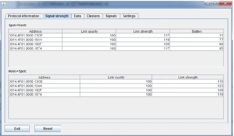
The second tab is “Signal strength” (Fig. 5.3).
The host application supports variety of Over-The-Air (OTA) commands, which can
be sent from a base station [13]. “Hello” command is one of them. It is used to discover the
sensors in the radio range of the base station (more information on the OTA commands can be
found in the Sun SPOT developer’s guide). It is possible to get a number of parameters about
current state of a sensor using this command. The upper table shows the link quality and
strength from a sensor node to the base station, while the bottom one shows the same
parameters, only from the base station to a sensor node. The battery level of a sensor is shown
as a percentage. Link Quality is uniquely determined by the CORR value: CORR is a
correlation measure provided directly by the radio part. Link Quality values range from 100%
(the best, corresponding to a CORR value greater than 100) to 0% (the worst, which means
the CORR value is less than 50) [13]. The signal strength value ranges from 1 (weakest) to
[image:29.612.114.514.469.702.2]121 (strongest). In order to convert this value to dB a user needs to subtract 106 from it.
29
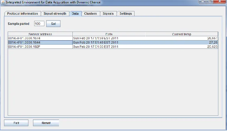
The third tab is “Data” (Fig. 5.4).
The table present in this tab consists of sensing data information: the address of a
sensor, date of last measurement and the sensing data itself – in this case it is temperature in
Celsius.
The sample period represents the time interval (in milliseconds) between two
successive temperature measurements. Also when using Radiogram protocol, the datagram
fits six samples, thus in order to increase efficiency of energy use and to increase the quality
of data (six measurements are better than one) the datagram will not be sent until it is full.
Therefore, even though the sample period is one value, when using Radiogram protocol, the
entry in the table will be updated six times slower. For example, if the sample period is set to
[image:30.612.129.497.327.542.2]one second, the measurements will arrive every six seconds.
Fig. 5.4. The “Data” tab of the framework.
This feature is not supported when using Radiostream protocol, because this protocol
opens a stream connection between two peers, instead of sending datagrams of certain fixed
size. Virtual sensors possess the same behavior as real sensors, so this is true for both real and
virtual sensors.
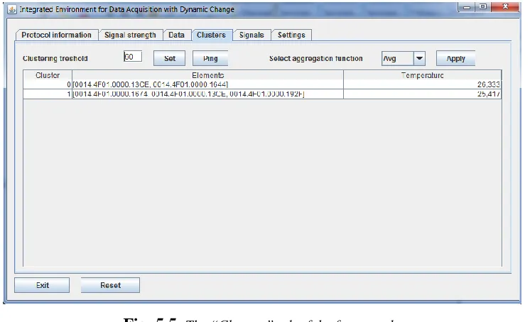
The next tab is “Clusters” (Fig. 5.5).
The table in this tab represents clusters to which sensors belong to. First column shows
30
temperature within the cluster, calculated with a certain aggregation function. The aggregation
functions implemented in the current version of IEDADC are the average and vote functions.
The value of the calculated temperature in a cluster is displayed when the sensors start
[image:31.612.128.501.138.365.2]sending their data to the base station.
Fig. 5.5. The “Clusters” tab of the framework.
The elements are put in a cluster according to the clustering threshold (measured in
dB), which can be customized at the top left of the panel. One element can be in several
clusters (details on how the clustering algorithm works can be found in section 5.2). Also the
aggregation function can be selected from the dropdown box on the right.
In IEDADC the “Ping” button has broader capabilities than sending a Hello command
OTA. Additionally, it calculates signal strengths between sensor nodes, clusters them and
draws a graph view of nodes according to the signal strengths between them (Fig. 5.6.1). It
also plots a graph of average current being drawn from the batteries (mA) with respect to the
time in minutes (Fig. 5.6.2). Section 5.2 provides details about this process.
The graph layout in this framework implements the Fruchterman-Reingold
force-directed algorithm for node layout3. Among the parameters that affect the graph layout are the attraction and repulsion multipliers. First multiplier determines how much the edges try to
keep their vertices together and the second multiplier determines how much the vertices try to
31
push each other apart. The graph represents the network where signal strength between nodes
is the weight of an edge in the graph and vertices are the sensor nodes.
Fig. 5.6.1. Graph view of the network. Vertices
have labels of last four characters of a sensor
node’s address. Weights of edges are the signal
strengths between two nodes.
Fig. 5.6.2. A graph of average energy use measured in
mA (y-axis) over time measured in minutes (x-axis).
Green line represents the use of the Radiogram
protocol, blue line represents the usage of
Radiostream protocol.
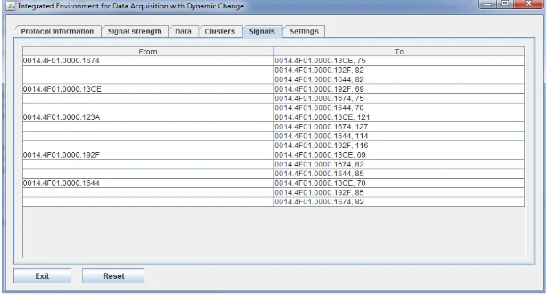
The “Signals” tab (Fig. 5.7) shows the signal strengths between nodes. The table
structure can be described in the following way: left column shows the node in point A and
right column shows the node in point B with the signal strength between these nodes. The
blank value in the left column means that the node in point A is the same. For example, in the
figure below, the node with the last four characters of its address being 1674 has signal
32 Fig. 5.7. The “Signals” tab of the framework.
The last tab, called “Settings” (Fig. 5.8) allows dynamic customization of the protocol
settings and switching protocols. A user may also define settings for triggering actions
automatically such as protocol switching, the period of network state information collection or
the condition for enabling the PEAS protocol.
[image:33.612.109.515.404.654.2]
33
For example, the degree of coverage can be customized in the PEAS protocol settings.
By default this value is set to one. However it is possible to increase this number to attain
higher accuracy through the “# of working sensors” filed. The second parameter we can
customize is the sleeping time duration (in seconds), which affects the frequency of probing
rate of sleeping sensors. The Probing range, the third parameter, determines the signal
strength threshold level used by probing and working sensors to determine whether to react to
the incoming messages.
The Controller settings bring some level of automatization to the process of the
interaction with WSN. The user can dynamically customize them by pressing the “Apply”
button. The settings are subdivided into two categories: periodic settings and conditional
settings. The first category lets the controller repeat commands after predetermined periods of
time, which are set in the corresponding text fields. The second category performs the
command only if a certain condition is satisfied. For example, it is possible to switch
protocols between Radiostream and Radiogram after every 300 seconds. The period of
switching can be changed in the text field next to the corresponding check box. The check box
“randomize” lets the period to be generated randomly within the range from the period text
box. This option brings some level of security to the WSN communication. Although the
security concepts are out of the scope of this work, this option enables random changing of
communications protocols, which in turn will make eavesdropping or man-in-the-middle
attacks more difficult. The use of this option can be later investigated in the future work.
Among other periodic settings is the option of periodically pinging the sensor nodes and
collecting data. Conditional settings include an option such as switching forwarding protocol
if the average battery discharge level exceeds the threshold value and enabling the PEAS
protocol if the average battery level of the sensors goes below the threshold value, which is
also set in the corresponding text field.
Moving slider only takes effect when the controller is running. Moving it from one
position to another triggers two commands: switching protocol from one to another and
enabling/disabling PEAS protocol. For example, when the slider is at the Radiogram position,
this means that the Radiogram protocol is currently in use. If it is moved to the Radiostream +
PEAS position, the protocol would first switch to the Radiostream and then PEAS protocol
would be enabled. If the slider is moved back to the Radiogram, the protocol would switch
34
The “Start” button at the bottom left corner of the panel starts the Controller. This
entails that the framework will analyze the incoming data and trigger the corresponding
actions automatically, specifically protocol switching, the period of network state information
collection or the condition for enabling the PEAS protocol. The framework logic in Section
5.2 describes this part in detail.
5.1.2 Model
The Model module is run on a host application, which resides on a computer. It is the
core part of the framework functionality. It is responsible for communicating with and
management of the sensor nodes. The Model provides an overall optimization of the WSN
operation against selected criteria. This way it assures the protocol adaptation to a particular
application by supporting dynamic protocol selection. In this module, all the information from
the sensor nodes is collected and analyzed. Based on this analysis, the Model may trigger
corresponding actions through the Controller component. All actions taken are constantly
reflected on the View, so the user can track down the behavior of the Model. The
management of a WSN involves maintaining the state information about the network on a per
node basis, such as the link status, state of a node (active or sleeping), battery level, and the
sensed data. Communication with the sensor nodes is the means by which the interaction
between the base station and the sensor network is established. The interaction includes
sending the commands to one or multiple nodes as well as retrieving the sensor network state
information or application specific data. Enabling plug-ins and dynamic protocol selection is
the key to flexibility and adaptation of the IEDADC to various WSN applications. Once the
network starts running, the protocol can be selected and the plug-in can be activated either by
a user or automatically, according to the user predefined setting. The plug-in can be
dynamically configured only by a directive from a user.
The model interacts with sensor nodes using the base station. Unlike the sensors,
which run J2ME applications, the host application is a regular J2SE program. In this
framework the base station operates in dedicated mode, meaning that it can be used only by
one application, within the same JVM [13]. As a result, the overall representation of the
network can be described as some number of sensor nodes sending information to a single
35
The model has references to the View module through the corresponding interface and
two other objects: one plots the graph of the average current being drawn from batteries and
the other plots the graph representation of the network (Fig. 5.9).
Fig. 5.9. The references between modules of the IEDADC.
When Model is initiated, it first checks if the base station is present. If true, then it
performs all other necessary initializations, such as creating references to above mentioned
objects. Then it broadcasts its availability and starts listening for the connection requests from
the sensor nodes. The sensor nodes, in turn, try to establish connection to the base station by
periodically broadcasting the request for connection. Once the base station receives the
request, it replies to that node and creates a listening thread for this particular sensor. There is
a separate thread for every sensor establishing connection to the model, including virtual
sensors (Fig. 5.9). When sensor node sends some message to the base station, it is processed
by the thread at the model, and then the message is sent to the corresponding method in the
Model. It also works in the opposite direction: the message sent to a particular node is sent
through the corresponding thread instead of broadcasting.
The Model module implements the localization and clustering algorithms. These
algorithms are provided as part of the QA mechanism of the framework. The clustering
algorithm is implemented in such a way that if the measurement of a sensor deviates by five
degrees Celsius from the measurements of other sensors in the cluster, then this node is
separated in a different cluster. This is done in order to avoid deviation of the calculated value
of a temperature in a cluster and to attract the attention of a user. This approach was inspired
by [16], where every data is given a flag of a certain color, where the green flag is given when
Proxy
Model
View listener
Model listener View
Controller Thread
Graph view
36
the data is “good”, i.e. there is no deviation from the overall measurements and the red flag
otherwise. The paper mentioned that if the data is given a red flag, it does not necessarily
mean that the data is wrong, it only lets the user know that the current data requires attention.
This approach is helpful in the case when there are two sensor nodes located close to each
other, but separated by a window – one measures the temperature indoors and the other one
measures the temperature outdoors, where the temperature can be significantly different.
Also the mechanism of switching the protocols is implemented in this module. The
model keeps track of which protocol is currently in use, so when switching protocol, the
model broadcasts corresponding command to the sensor nodes. Sensor nodes in their turn
reconnect to the base station. When the base station receives the request for connection from
the node to which it already has a connection, it removes the previous connection and creates
a new one with the new protocol in use. The reply message from the base station contains the
information about the protocol which should be used by the nodes.
The framework interaction with the sensor network can be represented as the
following (fig. 5.10). Upon a user’s command, the Model sends commands to the proxy
modules. The proxy modules control a sensor node’s operational mode and, possibly, send
back the reply. The plug-ins can influence the operation of a sensor node through interaction
with the proxy module. Sensor nodes can interact with each other when using miltihop routing
or probing the environment for locating working sensor nodes as part of the PEAS protocol
37 Fig. 5.10. IEDADC sensor network interaction overview.
Another feature of the Model is the support of virtual sensor nodes, which emulate the
behavior of real sensors. In this case no connection is created between a virtual sensor and the
base station. As before, a separate thread is created for each virtual sensor. A user can
manually set the parameters of the virtual sensor through the View module, such as the signal
strength to the base station, the temperature measurement, and the battery level of the sensor.
This information will be taken from the thread by the Model for analysis. Virtual sensor nodes
allow testing the behavior of algorithms implemented in the framework, such as the
localization and clustering algorithms.
5.1.3 Plug-in
The goal of the Plug-in module is to optimize a WSN operation for a particular
application by selecting certain parameter values. The plug-in parameters can be dynamically
customized by the directives from a user. For example, managing the degree of coverage of
the monitoring area by putting the redundant sensor nodes to sleep, keeping only necessary
38
This protocol is implemented as a part sensor application of the framework. However,
the parameters of the protocol, which affect its work, are configured from the GUI by a user.
The new parameter values are broadcasted from the base station to every sensor node.
The following parameters can be configured in this protocol.
As mentioned in section 2, sensor sleeps for exponentially distributed duration
generated according to a probability density function [21], where ts is the
sleeping time duration (measured in seconds) and λ is the probing rate – the frequency of a
sensor node probing the environment for a working node (measured in wake-ups per
seconds). There is also another parameter: λd – desired probing rate. Eventually, after some
time the λ will float around the desired rate, according to the proof provided in [21], with the
help of adaptive sleeping mechanism. These two lambdas are initialized when the protocol
starts. The reason for having two separate lambdas is that initially it is required to establish
working nodes as fast as possible, that is why the value of λ is higher than λd, so that the
network can start operating. The value of sleeping time duration ts directly affects the value of
the λ according to the formula: . Since the frequency of wake-ups is not needed to be
high after the working nodes are found, the value of λd,towards which the λis moving, is
calculated as: . The sleeping time duration parameter can be configured through the
View module.
Another parameter is the number of the working nodes. In order to increase the
accuracy of data, the number of working sensors within one region can be increased from one
to some number k. This parameter customizes the degree of coverage of the sensing area.
It is important to note that pseudorandom generators provided by Java programming
language only return us a uniformly distributed value within certain range. In order to
generate exponentially distributed values, the Inverse Transform Sampling formula is used:
Let , then ,
where λ is the probing rate, U is the uniformly distributed value between 0 (exclusive) and 1
(inclusive) and value of X is the generated sleeping time duration of a sensor node.
5.1.4 Proxy
The proxy is the IEDADC module that is run on a sensor node. It has three main
responsibilities:
![Fig. 3.5. Cluster-based WSN architecture [2].](https://thumb-us.123doks.com/thumbv2/123dok_us/51555.4710/23.612.167.458.57.293/fig-cluster-based-wsn-architecture.webp)