An evolutionary approach to the solution of multi-objective min-max problems in evidence-based robust optimization

(1)

An Evolutionary Approach to the Solution of Multi-Objective

Min-Max Problems in Evidence-Based Robust Optimization

Simone Alicino and Massimiliano Vasile

Abstract— This paper presents an evolutionary approach to solve the multi-objective min-max problem (MOMMP) that derives from the maximization of the Belief in robust design op-timization. In evidence-based robust optimization, the solutions that minimize the design budgets are robust under epistemic uncertainty if they maximize the Belief in the realization of the value of the design budgets. Thus robust solutions are found by minimizing, with respect to the design variables, the global maximum with respect to the uncertain variables. This paper presents an algorithm to solve MOMMP, and a computational cost reduction technique based on Kriging metamodels. The results show that the algorithm is able to accurately approximate the Pareto front for a MOMMP at a fraction of the computational cost of an exact calculation.

I. INTRODUCTION

G

IVEN the model of a system or process, the lower

expectation in the realization of the value of a particular performance index for that system or process can be defined as the degree of belief that one has in a certain proposition being true, given the available evidence. In the framework of imprecise probabilities, it can be seen as a lower bound to the cumulative distribution function of classical probability theory. Its use is therefore interesting in engineering design, as it gives the lower limit of the confidence that the design budgets under uncertainty will be below a given threshold. In this framework both epistemic and aleatory uncertainties can be treated even when no exact information on the probability distribution associated to a particular uncertain quantity is available. Stochastic variables, with associated probability, are replaced by a multivalued mapping from a collection of

subsets of an uncertain spaceU into an envelope defined by

the lower and upper expectation (Belief and Plausibility in the case of Evidence Theory) in the realization of a particular value.

In the preliminary design of an engineering system the type of uncertainty is often mainly epistemic in nature, as in a later stage of the design more information is generally available. It is therefore natural to assign belief masses to intervals of values rather than precise probabilities. The main drawback with the use of multivalued mappings is that the computation of the lower and upper expectations, Belief and Plausibility in the case of belief functions, has a complexity that is exponential with the number of un-certain variables. Recently, Vasile et al. [1] proposed some

Simone Alicino and Massimiliano Vasile are with the Depart-ment of Mechanical and Aerospace Engineering, University of Strath-clyde, Glasgow, United Kingdom (email: {simone.alicino, massimil-iano.vasile}@strath.ac.uk).

This work is partially supported by an ESA/NPI grant ‘Evidence-based Robust Design Optimization’

strategies to obtain an estimation of the maximum Belief with a reduction of the computational cost. The approach starts by translating an optimization under uncertainty into a single or multi-objective min-max problem equivalent to a worst-case scenario optimization problem. Although this approach avoids the intrinsic exponential complexity in the computation of the Belief, it still requires a high number of function evaluations. This paper presents an algorithm that implements special heuristics to increase the probability to find the exact global Pareto front in the case of a min-max problem on multi-modal functions. Also, it presents an approach based on Kriging surrogate models to reduce the computational cost associated to the solution of the MOMMP. The combination of evolutionary algorithms and surrogate models has been object of considerable research efforts in the last decade, as summarized in [2], [3]. How-ever, to the authors’ knowledge, not many papers deal with surrogate-based min-max optimization. Ideas of combining evolutionary optimization and surrogate modelling to solving min-max problems were proposed in [4], [5]. More recently Marzat et al. [6] proposed a non-evolutionary approach using Kriging metamodels to reduce the computational cost of the solution of single objective min-max problem in worst-case scenario optimization.

The approach proposed in this paper addresses specifically multi-objective min-max optimization problems and differs from previous work in the way the surrogate model interfaces with the optimization algorithm. As it will be shown, the ulti-mate goal is to build a surrogate of the maximization process. The paper starts with a brief introduction to Evidence Theory and its use in the context of robust design optimization in Section II. Section III introduces an algorithm to compute a multi-objective optimal design solution under uncertainty. Section IV explains the use of surrogate modelling to reduce the computational cost in multi-objective optimization cases. Section V presents the results on some scalable test cases that were applied to assess the performance of the proposed algorithm.

II. EVIDENCE-BASEDROBUSTDESIGNOPTIMIZATION

Evidence Theory (also known as Dempster-Shafer Theory) [7] allows to adequately model both epistemic and aleatory uncertainty when no information on the probability distribu-tions is available. For instance, during the preliminary design of an engineering system, experts can provide informed

opin-ions by expressing their belief in an uncertain parameter u

being within a certain set of intervals. The level of confidence

(2)

quantified by using a mass function generally known as Basic

Probability Assignment (bpa). Note that the bpa is a belief

rather than an actual probability. All the intervals form the

so-called frame of discernmentΘ, which is a set of mutually

exclusive elementary propositions. The frame of discernment can be viewed as the counterpart of the finite sample space

in probability theory. The power set ofΘis calledU = 2Θ,

or the set of all the subsets of Θ (the uncertain space in

the following). An element θ of U that has a non-zero bpa

is called focal element. When more than one parameter is uncertain, the focal elements are the result of the Cartesian product of all the elements of each power set associated to

each uncertain parameter. Thebpa of a given focal element

is then the product of the bpa of all the elements in the

power set associated to each parameter. All the pieces of evidence completely in support of a given proposition form

the cumulative belief functionBel, whereas all the pieces of

evidence partially in support of a given proposition form the

cumulative plausibility function P l. The BeliefBel and the

Plausibility P lfunctions are defined as follows:

Bel(A) = X

∀θi⊆A

m(θi) (1)

P l(A) = X

∀θi∩A6=0

m(θi) (2)

where A is the proposition about which Belief and

Plausi-bility need to be evaluated. For example, the proposition can be expressed as:

A={u∈U |f(u)≤ν} (3)

where f is the outcome of the system model and the

thresholdν is the desired value of a design budget (e.g. the

mass). Thus, focal elements intercepting the set A, but not

fully included in it, are considered in P l but not in Bel.

It is important to note that the set A can be disconnected

or present holes, likewise the focal elements can be discon-nected or partially overlapping.

An engineering system to be optimized can be modelled

as a function f : D ×U ⊆ <m+n _{→ <}_{. The function}

f represents the model of the system budgets (e.g. power

budget, mass budget, etc.), and depends on some uncertain

parametersu∈U and design parametersd∈D, whereDis

the available design space and U the uncertain space. What

is interesting for the designers is the value of the function

f for whichBel = 1, i.e. it is maximum. This value of the

design budget is the threshold νmax above which the design

is certainly feasible, given the current body of evidence. Ifq

objective functions exist, then the following problem can be solved without considering all the focal elements:

νmax= min

d∈DF= mind∈D[maxu∈U¯

f1(d,u), . . . ,max

u∈U¯

fq(d,u)]T

(4) Problem in 4 is a multi-objective min-max over the design

space D and the uncertain space U¯, where U¯ is a unit

hypercube collecting all the focal elements in a compact set

with no overlapping or holes. The transformation betweenU

andU¯ is given by:

xU =

bu_U,i−bl_U,i

bu_{U ,i}¯ −bl_{U ,i}¯

xU ,i¯ +b l U,i−

bu_U,i−bl_U,i

bu_{U ,i}¯ −bl_{U ,i}¯ b

l ¯ U ,i (5)

wherebu_U,i andbl_U,i(resp.bu_{U ,i}¯ andbl_{U ,i}¯ ) are the upper and

lower boundaries of thei−thhypercube to whichxU,i(resp.

x_{U ,i}¯ ) belongs.

III. A MULTI-OBJECTIVEMIN-MAXEVOLUTIONARY

ALGORITHM

Problem in 4 searches for the minimum of the maxima

of all the functions over U¯ and represents an example of

worst-case scenario design optimization. The maximum of every function is independent of the other functions and corresponds to a different uncertain vector. Therefore, all

the maxima can be computed in parallel with q

single-objective maximizations. The maximization of each function

is performed by running a global optimization overU¯ using

Inflationary Differential Evolution (IDEA). The minimization

over D is performed by means of MACSν, a modified

version of MACS2.

IDEA [8] is a population-based memetic algorithm for single-objective optimization. It hybridizes Differential Evo-lution and Monotonic Basin Hopping paradigms in order to simultaneously improve local convergence and avoid stagna-tion, as demonstrated for some space trajectory optimization problems.

MACS2 [9] is a memetic algorithm for multi-objective optimization based on a combination of Pareto ranking and Tchebycheff scalarization. The search for non-dominated solutions is performed by a population of agents which combine individualistic and social actions. The initial

pop-ulation is randomly generated in the search domain D.

Individualistic actions perform a sampling of the search space

in a neighborhood Nρ of each agent. Then, subsets of the

population perform social actions aiming at following partic-ular descent directions in the criteria space. Social agents im-plement a Differential Evolution operator and assess the new candidate solutions using Tchebycheff scalarization. Current non-dominated solutions are then stored in an archive. Both social and individualistic actions make use of a combination of the population and the archive.

MACSν is the min-max variant of MACS2. Indeed, in a

classical minimization problem two solutions d1 andd2 are

ranked according to which one gives the lower value of the function. In the minimization loop of a min-max problem, the same can be done only if the maximization loop has returned

the actual global maximau˜1andu˜2. However, this is usually

not true. Therefore a mechanism of cross-check such that

also (d1,u2) and (d2,u1) are evaluated is needed in order

to increase the probability that each maximization identifies the global maximum and correctly rank two solutions. For

this reason, MACSν (see Algorithm 1) endows MACS2

(3)

dominant. A cross check is necessary to compare the values of the objective functions for a newly generated design vector against the function values of an already archived solution. Consider, in fact, that a different design vector corresponds in general to a different landscape of the objective functions, and therefore to a different location of the maxima. More-over, the cross-check performs a local search or a simple function evaluation in the inner maximization loop depending on whether the location of the maxima changes or not, respectively, for different design vectors.

At the end of this cross-check, Algorithm 3 is run to select the design vectors to attribute to the next generation, once a new candidate population is generated after either individualistic or social moves. The following heuristics are

implemented: ifd(resp.u) is unchanged, the oldu(resp.d)

is replaced with the new one, if it yields a better value of

the objective function; if bothdanduare different, the new

vectors will replace the old ones.

A validation (see Algorithm 4) is run at the last iteration of

MACSν, after the individualistic and social moves have been

performed. It performs a global search for the extremes in the archive, and replaces the corresponding uncertain vector and objective if the new ones give a better value of the objective function, until there is no more variation in the extremes of the archive. This step is introduced to mitigate the possibility

that the cross-check operators assign the same incorrectuto

alld vectors in the population and archive.

A. Optimization Performance Metrics

In order to assess the Pareto frontf found by MACSνwith

respect to a reference front g, we made use of convergence

Mconv (Equation 6), and spreading Mspr (Equation 7),

defined as:

Mconv= 1

Np Np

X

i=1 min j∈Mp

100

gj−fi

gj

(6)

Mspr = 1

Mp Mp

X

i=1 min j∈Np

100

fj−gi

gi

(7)

whereNp andMp are the cardinality of the frontsf andg,

respectively. As one can see, the lower the value of Mconv

andMspr, the better convergence and spreading, respectively.

In addition, two performance indexes pconv =P(Mconv <

tconv) and pspr = P(Mspr < tspr) compute the success

rate with respect to some thresholds tconv and tspr. These

indexes tell how many times, over a certain number of runs, convergence and spreading are equal to or below such thresholds.

IV. SURROGATEMODELLING

The solution of the min-max problem involves an increase in the number of times the objective function needs to be evaluated. In this context, the use of surrogate models can play a valuable role. The surrogates are constructed using data drawn from high-fidelity models, and provide fast approximations of the objectives at new design points. In this

Algorithm 1 MACSν

1: Initialize population P, archive A = P, nf eval = 0,

= 0.7,δ= 10−6

2: whilenf eval< nf eval,max

3: Run individualistic moves and generate trial

popula-tion Pt

4: for all d∈Pt 5: for all darch∈A

6: if ddarch

7: CROSS-CHECK(Pt, A) .Alg. 2

8: end if

9: end for

10: end for

11: MIN-MAXSELECTION(P, Pt) .Alg. 3

12: Update P andA

13: Z ← kFmax_arch−Fmin_archk

14: Run social moves and generate candidate population

Ps

15: for all d∈Ps 16: for all darch∈A

17: if ddarch orkF(d)−F(darch)k> Z

18: CROSS-CHECK(Ps, A) .Alg. 2

19: end if

20: end for

21: end for

22: MIN-MAXSELECTION(P, Ps) .Alg. 3

23: Update P andA

24: VALIDATION(A) .Alg. 4

25: for all d∈P

26: for all darch∈A

27: if ddarch ord≺darch

28: CROSS-CHECK(P, A) .Alg. 2

29: else ifkF(d)−F(darch)k< δ

30: Replace u∈P withu∈A

31: end if

32: end for

33: end for

34: Fit surrogate model inD with the elements of A

35: end while

paper we propose an approach in which a surrogate is built

in theD space only, as shown in Figure 1(a). The surrogate

in the design space hasd as design sites, andg as response,

and is therefore constructed and updated in the outer loop of

the optimization, i.e. the minimization over D.

The approach can be formalized as follows. Let us con-sider, without loss of generality, Problem 4 in the single-objective case:

νmax= min

d∈Dmaxu∈_U¯ f(d,u) (8)

This can also be written as

νmax= min

d∈Dg(d,u) (9)

where

g(d,u) = max

u∈U¯

(4)

Algorithm 2 Cross-check

1: functionCROSS-CHECK(P, A)

2: for alll∈ {1, . . . , q}

3: if kul_arch−ulk 6= 0

4: Compute local maxima ˜ul_arch and˜ul

associ-ated todanddarch

5: iffl_(darch_,_˜_ul

)≥fl_(darch_,_ul arch)

6: replace ul

arch withu˜ l

7: end if

8: iffl(d,˜uarchl )≥fl(d,ul)

9: replace ul _with_˜_ul

arch

10: end if

11: end if 12: end for 13: returnP, A

14: end function

Algorithm 3 Min-Max Selection

1: functionMIN-MAXSELECTION(P, Pnew) 2: for alll∈ {1, . . . , q}

3: for all (d∈P)S_(dnew

∈Pnew) 4: ifkdnew−dk= 0

5: if fnewl (dnew,unewl )≥fl(d,ul)

6: replaceul _with_ul

new

7: replacefl withfnewl

8: end if

9: else ifkdnew−dk>0

10: if fl

new(dnew,ulnew)< fl(d,ul)

11: replaced withdnew

12: replacefl withfnewl

13: end if

14: end if

15: end for

16: end for 17: returnP

18: end function

i.e. it is the result of the inner loop of the optimization. The aim of this approach is to separate the outer and inner loops. The idea behind this is that the inner loop can be

called only if the surrogate(d, g)needs to be updated. If the

accuracy of the surrogate(d, g)is above a certain threshold,

only the outer loop is run, hence saving computational expense. In addition, such approach allows the surrogate model to be dependent only on the relevant parameters, i.e.

the design vectord for the outer loop (Figure 1(b)).

The surrogate model is built by using the archived solu-tions of the minimization loop as design sites (see Algorithm 1). The surrogate is therefore built and updated only if there are new elements in the archive. Note that a strategy that would build the surrogate progressively as new agents are deployed into the minimization loop, therefore using all the design solutions is not applicable because the design solutions need to be cross-checked. Without these steps, the surrogate would contain design solutions that, while being

Algorithm 4 Validation

1: functionVALIDATION(A)

2: for alll∈ {1, . . . , q}

3: ∆fbest= 1 4: while∆fbest6= 0 5: j= argminfl∈A

6: Run global optimization overU¯ and compute

newf¯l_{and associated} _¯_ul

7: iff¯l_{> f}l

8: replace ul_∈_A_with_u_¯l

9: replace fl_∈_A_with_f¯l

10: ∆fbest= ¯fl−fl

11: end if

12: end while 13: end for 14: returnA

15: end function

f

g1

u1 Ū

g

g1 (u1)

D dopt

d₁

ν_max

(a)

SURR. D

MAX U e > tol e < tol

d

fsurr, Ø f, u

f

(b) Fig. 1

(A) CONCEPTUAL EXAMPLE OF THE SURROGATE MODELLING STRATEGY. THE PLOT REPRESENTS THE SURROGATE IN THEDSPACE. THE DOTS ARE THE DESIGN SITES. NOTICE THATg1= max

u f(d1, u). (B) SCHEMATIC OF THE SURROGATE MODELLING STRATEGY.

non-dominated, do not maximize the inner loop. A further feature of our technique is that the number of design sites

is kept below a user-specified threshold of ns points. Once

the number of sample points overcomes such threshold, the sites to be retained are chosen so that the spreading of the Pareto front is maximized, and the members of the archive evenly distributed. By noting that the design sites are, as explained in the previous paragraph, the current archive of Pareto set and front, therefore one can define a sector in the criteria space defined by the origin and the extrema of

the front. Then, such sector is divided into ns−1 smaller

sectors of equal angle, and the design sites to be retained

are the ns ones which distance to the boundaries between

the sectors is minimum. This allows for the surrogate to approximate accurately the current Pareto front, and also to keep the surrogate to a reasonable size.

A. Kriging Predictor

(5)

use of a regression function and a correlation model to predict the response of a function at a desired point. Being an interpolation method, it gives an exact prediction of the response at the sample points. Moreover, it assumes that the output function values are correlated in design space, i.e. closer points are more highly correlated. A complete derivation of the Kriging model can be found in Jones [10].

If we suppose to have a set of n design sites (x,y), the

correlation matrix R of the design points can be expressed

as

R= [Rij] = exp

"

−

d

X

l=1

θlkxil−xjlkpl

#

(11)

where i, j = 1, . . . , n. In the same way, the correlation of

the new point x∗ at which we want to predict the response

ˆ

y(x∗), with the design points can be expressed as

r= [ri] = exp

"

−

d

X

l=1

θlkx∗l −xilk pl

#

(12)

The correlation model depends on two parameters θ andp.

They can be found to be the ones that minimize the mean

squared error between the predicted responseyˆand the actual

response y. Therefore an optimization is to be performed

during the training phase. Under the assumption that the regression function is a zero-th order polynomial, i.e. it is

an×1vector of ones 1, the predictionyˆ(x∗)can be found

to be

ˆ

y(x∗) = ˆµ+rTR−1(y−1ˆµ) (13)

where

ˆ

µ= 1 T_R−1_y

1TR−11 (14)

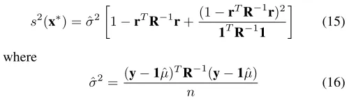
One of the key benefits of Kriging is the provision of an estimated error of its predictions. The estimated mean squared error (MSE) for a Kriging model is

s2(x∗) = ˆσ2

1−rTR−1r+(1−r

T_R−1_r)2 1TR−11

(15)

where

ˆ

σ2= (y−1ˆµ) T_R−1

(y−1ˆµ)

n (16)

is the estimated variance.

The availability of an estimate of the prediction error is a very convenient feature, as it can be exploited in the surrogate

update strategy. Letting ymin be the current best function

value, and Y(x) a random variable normally distributed,

with mean yˆ(x) and standard deviation s(x), describing the

uncertainty about the function’s value, an improvement I

is achieved if I(x) = ymin−yˆ(x) > 0. In this paper we

consider a method based on the probability of improvement, that is deemed to be one of the best two-stage methods to the Kriging update [10] [11]. The main advantage of this method is that the probability of improvement is independent of magnitude and units of the function value.

The probability of an improvement is the area of the PDF,

with meanyˆ(x)and standard deviations(x), calculated from

ymin to−∞. That is

P(I(x)) = Φ (u(x)) (17)

whereΦis the normal cumulative distribution function, and

u(x) =ymin−yˆ(x)

s(x) =

I(x)

s(x) (18)

One can set a thresholdτon this probability of improvement,

and update the Kriging predictor ifP(I)≥τ. The advantage

of such method is that the threshold τ is a simple

non-dimensional probability measure, therefore independent of the magnitude and units of the function value.

The probability of improvement can be extended to the case of multiple objectives. In this case, an improvement is achieved when the new point dominates at least one member of the archived non-dominated points. Considering

two uncorrelated objectives, the improvement I(x) is then

defined as y1P −yˆ1(x)>0 ∪ y2P−yˆ2(x)>0, where

y1P and y2P represent the members of the archived Pareto

front. If the Pareto front is composed of NP members, by

defining

ui₁(x) = y i

1P−yˆ1(x) s1(x)

, ui₂(x) = y i

2P−yˆ2(x) s2(x)

(19)

for i= 1, ..., NP, the probability of improvement is

P(I(x)) = Φ u11(x)

+ NP−1

X

i=1

Φ ui₁+1(x)−Φ ui1(x)

×Φ ui₂+1(x)

+h1−ΦuNP

1 (x) i

ΦuNP

2 (x)

(20)

This expression can be obtained by integrating the Gaussian

distribution underlying the improvement I for the two

ob-jective functions between −∞and the Pareto front [12].

V. TESTCASE

[image:5.612.50.300.503.578.2]

The surrogate-based optimization algorithm described in the previous sections was tested on six bi-objective test cases. The chosen functions, reported in Table I, have the property of being easily scalable. More in detail, functions MV9, MV10, and EM1 present very challenging landscapes, with multiple maxima that can change significantly with the design vector. Function MV10, in particular, is characterized by having the maxima located on top of multiple sharp, steep peaks. The six test cases are composed of the functions in Table I as reported in Table II. The dimension of the design

vectord, as well as the uncertain vectoru, is 8, for a total of

(6)

TABLE I TEST FUNCTIONS.

Function Parameters

MV1 f=Pn i=1diu2i

d∈[1,5]n

u∈[−5,3]n MV2 f=Pn

i=1(di−ui)2

d∈[1,5]n

u∈[−5,3]n MV3 f=

Pn

i=1(5−di) (1 + cosu1) + d∈[1,5]n + (di−1) (1 + sinui) u∈[−5,3]n MV8 f=Pn

i=1(2π−ui) cos (ui−di) d∈[0,3] n

u∈[0,2π]n MV9 f=Pn

i=1(di−ui) cos (−5ui+ 3di) d∈[1,3] n

u∈[−π 2 ,

3π

2]

n MV10 f=

Pn

i=1(di+ui)× d∈[−4,2π]n

cos (−ui(5|d|+ 5) + 3di) u∈[π,2π]n EM1 f=Pn

i=1(ui−3di) sinui+ (di−2)2

d∈[0,2π]n

u∈[0,20]n

vs. outer loops, total number of agents and number of social

agents for MACSν, and F vs. CR for IDEA. Note that,

as shown in [9], F and CR of MACSν do not have a

big impact. The sensitivity analysis was run for test case TC4. The results were assessed in terms of success rate of finding the global maximum in the inner loop, indicated

as s.r.(fi), as well as convergence and spreading as per

Equations 6 and 7. Results in Tables III - V show that the best success rate, convergence, and spreading are obtained for 20

agents for MACSν, half of which perform the social actions,

and F = 1, CR = 0.1 and 200n function evaluations for

IDEA. The Kriging predictor makes use of a zero-th order polynomial regression function and a Gaussian correlation function. The number of design sites is kept below 20. Three thresholds for the surrogate update have been tested, and they were set to 0.3, 0.5 and 0.9, i.e. 30%, 50% and 90% probability of improvement. The reference solution, i.e. the real front in Figures 2 - 4, was computed by merging the results of 200 runs of the same problem without using the surrogate model and with a number of function evaluations of

106_{. Tables VI to VIII summarize the performance metrics of}

the surrogate-based optimization for the six test cases at the several thresholds for the surrogate update. The results are the average performances obtained from the 200 runs needed to achieve a confidence interval of 95% on the success rate

being within a ±5% interval containing its estimated value

[8]. The columnInner/Outercontains the percentage of times

that the inner loop was called. The columns Mconv and

Mspr contain the mean value and, in brackets, the standard

deviation of Mconv and Mspr respectively. The columns

pconvandpspr contain the success rate of computing a front

which convergence and spreading are below the thresholds

tconv andtspr, that for this paper were set equal to 5 and

10, respectively.

From Tables VI to VIII it can be seen that the inner loop is called progressively less times as the surrogate update threshold increases, as expected. However, there is a variability among the test cases for the same thresholds. This is due to the fact that certain functions are more or less complicated to approximate by the surrogate model. Note also that there is little difference in the percentage of

TABLE II TEST CASES.

Test Case Function n

TC1 f1= MV1,f2= MV3 8

TC2 f1= MV2,f2= MV8 8

TC3 f1 = MV2,f2 = EM1 8

TC4 f1= MV8,f2= MV9 4

TC5 f1 = MV8,f2 = EM1 4

TC6 f1= MV10,f2= MV9 4

TABLE III

SENSITIVITY OF THE ALGORITHM TO THE NUMBER OF AGENTS

s.r.(f1, f2) Total agents

(Mconv, M spr) 5 10 20

Social/total

1/3 (100, 46.1) (100, 42.5) (100, 46.9)

(4.5, 6.8) (3.9, 5.9) (2.6, 4.8)

1/2 (100, 44.1) (100, 41.4) (100, 46.3)

(4.6, 6.7) (3.9, 6.1) (2.7, 5.0)

1 (100, 38.8) (100, 40.2) (100, 50.7)

(5.1, 7.9) (3.9, 6.1) (2.5, 4.7)

calls to the inner loop when the surrogate update threshold passes from 50% to 90%. This is an indication that the surrogate is able to approximate well the functions, and therefore there are only few points where the probability of improving the surrogate is above 0.9. By and large, the

surrogate-based MACSν produces good results for all the

test cases when the surrogate update threshold is 30%, with a computational saving of about 10%. Increasing the update threshold obviously causes the computational saving to be higher, as high as 50% for some cases, because less points are found that have 50% probability of improving the surrogate. This also causes a decrease of the quality of the results in terms of both convergence and spreading. Nevertheless, the solution found is good for four of the six test cases. When the surrogate update threshold is pushed as high as 90%, performances, as well as computational saving, only slightly

TABLE IV

SENSITIVITY OF THE ALGORITHM TOFANDCRIN THE INNER LOOP

s.r.(f1, f2) F

(Mconv, M spr) 0.1 0.5 1 2

CR

0.1 (99.9, 31.2) (100, 41.4) (100, 46.6) (99.9, 37.8)

(5.5, 7.0) (3.9, 6.1) (3.1, 5.3) (4.5, 6.4)

0.5 (100, 27.3) (100, 31.9) (100, 36.2) (100, 30.5)

(6.4, 8.1) (5.6, 7.3) (4.2, 6.3) (5.4, 6.9)

0.9 (100, 23.8) (100, 23.6) (100, 27.8) (100, 22.7)

(8.5, 9.5) (7.6, 8.4) (6.2, 7.6) (8.3, 9.0)

TABLE V

SENSITIVITY OF THE ALGORITHM TO THE NUMBER OF FUNCTION EVALUATIONS

s.r.(f1, f2) Outer loop

(Mconv, M spr) 1e5 2e5 3e5 4e5

Inner

loop

50n (100, 19.5) (100, 23.1) (100, 23.9) (100, 25.2)

(6.7, 9.4) (6.9, 8.7) (7.7, 9.1) (6.7, 7.8)

100n (100, 33.3) (100, 35.3) (100, 35.7) (100, 41.4)

(3.5, 7.0) (3.9, 6.5) (4.0, 6.3) (3.9, 6.1)

100n (100, 50.6) (100, 54.1) (100, 59.9) (100, 60.0)

(7)

[image:7.612.52.301.190.274.2]

TABLE VI

PERFORMANCE METRICS FOR SURROGATE UPDATE THRESHOLD OF30%.

Test Case Inner/Outer Mconv Mspr pconv pspr TC1 99.1% 1.4(0.8) 9.9(5.4) 100% 60% TC2 92.4% 0.8(0.1) 3.9(1.5) 100% 100% TC3 87.9% 0.7(0.3) 3.6(1.9) 100% 100% TC4 89.2% 2.4(1.5) 4.1(1.2) 96% 100% TC5 92.6% 2.6(2.4) 1.9(1.1) 90% 100% TC6 87.0% 3.8(0.8) 11.0(4.9) 95% 51%

TABLE VII

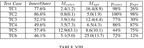
TABLE VIII

decrease with respect to the 50% threshold.

The Pareto fronts for the six test cases are shown in Figures 2 to 4 for the three surrogate update threshold of 30%, 50% and 90%. It can be seen that, as mentioned, the surrogate-based optimization algorithm is able to correctly identify the Pareto front for test cases TC2, TC3, TC5, and TC6. Test case TC4 presents a disconnected front, and while the region in the objective space where the real front lies could be identified, the surrogate-based algorithm could not identify the disconnected portions of the front. Test case TC1 proved to be more challenging to solve. Note that some points in the fronts seem to dominate the real solutions. Such points derive from an imperfect approximation by the surrogate.

VI. CONCLUSION

An algorithm for surrogate-based multi-objective worst-case optimization has been presented. The algorithm, called

MACSν, has the peculiarity of performing a number of

checks and cross checks to increase the probability to find the global optimum. In this paper, the optimization algo-rithm is coupled with surrogate modelling. The aim is to create a surrogate model that approximates the mapping between design parameters and function values, so that the expensive inner loop of the min-max algorithm is called only a fraction of the times. The algorithm was tested on six challenging bi-objective test cases made of scalable test functions, presenting multiple maxima and some of them disconnected fronts. An analysis of sensitivity of the parameters of the algorithm was carried out, showing how

several combinations of total vs. social agents,F vs.CR, and

number of function evaluations affected the performance of the algorithm. Moreover, three surrogate update thresholds were testes. The results were good for four out of six test cases, with a good approximation of the real Pareto front obtained with a computational cost of 50% of the exact one. In the case of disconnected fronts, the computed front lays on the real one, though the disconnected portions of the front where not identified. However, this study is limited to the use of the probability of improvement as surrogate update strategy. Other techniques, such as the expected improve-ment, were proposed in the framework of surrogate-based

optimization, and their use in conjunction with MACSν is

under investigation. A real case application of MACSν is

the maximization of Belief function, which finds importance in engineering robust design, for example, as it gives the value of the design budgets for which the design is certainly feasible under uncertainty.

ACKNOWLEDGMENTS

The Kriging predictor used for this work is the one implemented in the DACE Toolbox by Nielsen,

Lophaven and Sondergaard, and freely available at

http://www2.imm.dtu.dk/ hbni/dace/. The authors would like to thank the anonymous reviewers for helping to improve the quality of the paper. This work is partially supported through an ESA/NPI grant ‘Evidence-based Robust Design Optimization’.

REFERENCES

[1] M. Vasile, E. Minisci and Q. Wijnands, “Approximated Compu-tation of Belief Functions for Robust Design Optimization,” 53rd AIAA/ASME/ASCE/AHS/ASC Structures, Structural Dynamics, and Materials Conference, Apr. 2012.

[2] M. Bhattacharya, “Surrogate based Evolutionary Algorithm for Design Optimization,”World Academy of Science, Engineering and Technol-ogyvol. 1, 2007

[3] Y. Jin, “Surrogate-Assisted Evolutionary Computation: Recent Ad-vances and Future Challenges,”Swarm and Evolutionary Computation

vol. 1, pp 61-70, 2011

[4] A. Zhou and Q. Zhang, “A Surrogate-Assisted Evolutionary Algorithm for Minimax Optimization,”2010 IEEE Conference on Evolutionary Computation (CEC 2010), Jul. 2010.

[5] Y.-S. Ong, P. B. Nair, K. Y. Lum, “Max-Min Surrogate-Assisted Evolutionary Algorithm for Robust Design,”IEEE Trans. Evol. Comp.

vol. 10, pp 392-404, 2006

[6] J. Marzat, E. Walker and H. Piet-Lahanier, “Worst-case Global Opti-mization of Black-Box Functions through Kriging and Relaxation,”J. Global Optim.vol. 55, pp. 707-727, 2013.

[7] G. Shafer,A Mathematical Theory of Evidence.Princeton University Press, Princeton, NJ, 1976.

[8] M. Vasile, E. Minisci and M. Locatelli, “An Inflationary Differential Evolution Algorithm for Space Trajectory Optimization,”IEEE Trans. Evol. Comp.vol. 15, pp. 267-281, Apr. 2011.

[9] F. Zuiani and M. Vasile, “Multi Agent Collaborative Search Based on Tchebycheff Decomposition,” Computational Optimization and Applications, March 2013, DOI 10.1007/s10589-013-9552-9. [10] D. R. Jones, “A Taxonomy of Global Optimization Methods Based on

Response Surface,”J. Global Optim.vol. 21, pp. 345-383, 2001. [11] A. I. J. Forrester and A. J. Keane, “Recent Advances in

Surrogate-based Optimization,”Prog Aerosp Sci.vol. 45, pp. 50-79, 2009. [12] A. J. Keane, “Statistical Improvement Criteria for Use in

(8)