City, University of London Institutional Repository
Citation
:
Chen, T. & Zeng, Y. (2009). Classification of traffic flows into QoS classes by unsupervised learning and KNN clustering. KSII Trans. on Internet and Information Systems, 3(2), pp. 134-146. doi: 10.3837/tiis.2009.02.001This is the published version of the paper.
This version of the publication may differ from the final published
version.
Permanent repository link:
http://openaccess.city.ac.uk/8212/Link to published version
:
http://dx.doi.org/10.3837/tiis.2009.02.001Copyright and reuse:
City Research Online aims to make research
outputs of City, University of London available to a wider audience.
Copyright and Moral Rights remain with the author(s) and/or copyright
holders. URLs from City Research Online may be freely distributed and
linked to.
City Research Online: http://openaccess.city.ac.uk/ [email protected]
The research was partially supported by the U.S. National Science Foundation when Yi Zeng was previously at Southern Methodist University, Dallas, Texas, USA.
DOI: 10.3837/tiis.2009.02.001
Classification of Traffic Flows into QoS
Classes by Unsupervised Learning and KNN
Clustering
Yi Zeng1 and Thomas M. Chen2
1San Diego Supercomputer Center, University of California
San Diego, CA 92093 - USA [e-mail: [email protected]]
2
School of Engineering, Swansea University Swansea, Wales SA2 8PP – UK [e-mail: [email protected]] *Corresponding author: Thomas Chen
Received Mach 5, 2009; revised March 25, 2009; accepted April 10, 2009; published April 25, 2009
Abstract
Traffic classification seeks to assign packet flows to an appropriate quality of service (QoS) class based on flow statistics without the need to examine packet payloads. Classification proceeds in two steps. Classification rules are first built by analyzing traffic traces, and then the classification rules are evaluated using test data. In this paper, we use self-organizing map and K-means clustering as unsupervised machine learning methods to identify the inherent classes in traffic traces. Three clusters were discovered, corresponding to transactional, bulk data transfer, and interactive applications. The K-nearest neighbor classifier was found to be highly accurate for the traffic data and significantly better compared to a minimum mean distance classifier.
1. Introduction
N
etwork operators and system administrators are interested in the mixture of traffic carriedin their networks for several reasons. Knowledge about traffic composition is valuable for network planning, accounting, security, and traffic control. Traffic control includes packet scheduling and intelligent buffer management to provide the quality of service (QoS) needed by applications. It is necessary to determine to which applications packets belong, but traditional protocol layering principles restrict the network to processing only the IP packet header.
Deep packet inspection (DPI) can classify traffic by examining and decoding the higher layer protocols carried within packet payloads. The protocol field in the IP packet header will indicate the transport layer protocol (usually TCP or UDP); then the port numbers in the TCP/UDP header will indicate the application layer protocol if the port numbers are well-known. However, DPI has major drawbacks that limit its usefulness. If the packet payload is encrypted, the TCP/UDP header will be unreadable. Some applications, notably peer-to-peer protocols, do not use well-known or even predictable port numbers. In addition, some believe that DPI is an invasive technology that raises privacy issues.
Research in traffic classification has searched for methods to determine the composition of traffic, without recourse to examining the packet payload. For the purpose of traffic control, it is not necessary to classify individual packets as to their specific application; this would require detailed knowledge of all application layer protocols. The usual goal is more modest. Traffic flows are classified into a number of QoS classes, where flows within the same QoS class share similar QoS requirements. The fundamental idea of traffic classification is to differentiate flows based on flow and packet statistics that can be easily observed without examining payloads. Routers and switches with NetFlow or sFlow capabilities can collect traffic flow statistics, such as flow duration, number of packets and bytes, and packet length statistics. Our aim is to make use of the collected flow statistics to determine the QOS requirements for each flow.
There are three major research issues in flow classification. First, which flow statistics are the most useful features for differentiating flows? We could use as many statistics as possible but in practice, it is preferable to minimize the feature set by ignoring features that contribute little. In this paper, we investigate the usefulness of several features in four hour-long traffic
traces. Second, what are the QoS classes? They could be decided either a priori or preferably
without a priori assumptions using unsupervised clustering algorithms to discover the QoS
classes naturally inherent in traffic data. We experimented with unsupervised clustering using self-organizing map and K-means clustering. Third, how will new flows be classified into QoS classes? Many machine learning techniques such as neural networks, Bayesian classifier, and decision trees are possible. We compare K-nearest neighbor with minimum mean distance classification.
In Section 2, we review the previous work in traffic classification. Section 3 addresses the question of useful features and number of QoS classes. We describe experiments with unsupervised clustering of real traffic traces to build classification rules. Given the discovered QoS classes, Section 4 presents experimental evaluation of classification accuracy using k-nearest neighbor compared to minimum mean distance clustering.
Research in traffic classification, which avoids payload inspection, has accelerated over the last five years. It is generally difficult to compare different approaches, because they vary in the selection of features (some requiring inspection of the packet payload), choice of supervised or unsupervised classification algorithms, and set of classified traffic classes. The wide range of previous approaches can be seen in the comprehensive survey by Nguyen and
Armitage [1]. Further complicating comparisons between different studies is the fact that
classification performance depends on how the classifier is trained and the test data used to evaluate accuracy. Unfortunately, a universal set of test traffic data does not exist to allow uniform comparisons of different classifiers.
A common approach is to classify traffic on the basis of flows instead of individual packets.
Trussell et al. proposed the distribution of packet lengths as a useful feature [2]. McGregor et
al. used a variety of features: packet length statistics, interarrival times, byte counts,
connection duration [3]. Flows with similar features were grouped together using EM
(expectation-maximization) clustering. Having found the clusters representing a set of traffic classes, the features contributing little were deleted to simplify classification and the clusters were recomputed with the reduced feature set. EM clustering was also studied by Zander,
Nguyen, and Armitage [4]. Sequential forward selection (SFS) was used to reduce the feature
set. The same authors also tried AutoClass, an unsupervised Bayesian classifier, for cluster
formation and SFS for feature set reduction [5].
Roughan et al. experimented with k-nearest neighbor (KNN) and linear discriminant analysis (LDA) to classify flows into four QoS classes: interactive, bulk data, streaming, and
transactional [6]. This was an example of supervised classification where the number of
classes is known. Their chosen features included packet length statistics, flow rate, flow duration, number of packets, interarrival times, and TCP connection statistics. The main features were connection duration and mean packet length. In comparison, we do not decide
on QoS classes a priori. We discover a set of QoS classes using unsupervised clustering.
Moore and Zuev employed supervised Naive Bayes classification of flows into several
classes [7]. Their features included flow duration, TCP port number, interarrival times,
payload sizes, and effective bandwidth. While Naïve Bayes classification achieved 65 percent accuracy for real Internet traffic, the accuracy increased to 93 percent with the combination of kernel density estimation and 94 percent when Naïve Bayes was combined with FCBF (fast correlation-based filter). A later study followed up on Bayesian classification with a more
detailed discussion of features [8]. Ten, of a large set of features, were chosen as the most
useful. Unfortunately, the features include TCP header fields that require inspection of packet payloads. In comparison, our approach does not use TCP/UDP header fields, since they reside in the packet payloads.
BLINC followed a different approach to examine flow patterns to classify the behavior of
hosts on three levels: social, functional, and application [9]. Only flow statistics are used
without payload inspection. Empirically observed flow patterns are represented in “graphlets,” and host behaviors are classified by matching their traffic to the closest graphlet. Our goal differs from that of BLINC. Whereas BLINC uses traffic patterns to characterize hosts, our goal is to characterize each traffic flow in terms of its QoS requirements.
Bernaille et al. suggested that flows could be classified based on the first five packets [10]. The packet lengths constitute a vector, and similar vectors are grouped by k-means clustering. The study aim was to find a minimum number of packets to reasonably classify a flow.
Williams et al. compared five machine learning algorithms and concluded that Bayes
chosen a priori. Analysis of 22 features concluded the most useful features to be: number of packets in the flow (minimum, maximum, and mean), protocol (TCP or UDP), interarrival time (minimum, maximum), and flow duration. In contrast, our approach includes a data exploration phase, where the traffic classes are learned by unsupervised clustering.
Erman et al. compared unsupervised clustering algorithms: k-means, DBSCAN, and
AutoClass [12]. A later study used k-means clustering with 25 features that were reduced to:
number of packets, mean packet length, mean payload size, number of bytes, flow duration,
and mean interarrival time [13]. K-means clustering was also tried by Yingqiu et al. [14]. Our
methodology differs in that unsupervised clustering is used for data exploration to discover an inherent set of traffic classes in the data, and then supervised clustering is used for flow classification.
Crotti et al. proposed the idea of a “protocol fingerprint” characterized by three flow
statistics: packet length, interarrival time, and arrival order [15][16]. The proximity of a flow
to a protocol fingerprint is measured by the anomaly score.
NetADHICT used a divisive hierarchical clustering algorithm [17]. After clusters are
determined, packets are classified by decision trees based on features called (p,n)-grams.
These are substrings at fixed offsets within packets (p is the offset and n is the length of the substring). The NetADHICT algorithm finds and groups packets containing similar bit patterns. The approach fundamentally differs from our approach that assumes packets are already associated into flows and uses flow statistics for classification into QoS classes.
Decision trees were also investigated by Cao et al. to differentiate BitTorrent, HTTP,
SMTP, and FTP flows [18]. Their traffic data was limited to these four specific applications,
whilst our data contain a much wider range of applications.
In a different direction from clustering approaches, Wright et al. proposed the use of
hidden Markov models for packet lengths and times [19]. Similarly, Dainotti et al. use hidden
Markov models for joint distributions of packet payload size and interarrival time [20].
3. Unsupervised Clustering
3.1 Self-Organizing Map
We start with minimal assumptions and make no a priori assumptions about classes and
features to build classification rules. Some researchers have called this exploratory phase of traffic analysis, unsupervised clustering or off-line classification. The goal of unsupervised clustering is to discover the inherent classes in the traffic and secondarily to discover the most useful features for classification. Using a large set of features leads to high complexity and computation costs that may be unnecessary. Often some features little affect classification and can be ignored with no loss of accuracy.
We analyzed traffic data with two unsupervised clustering algorithms, self-organizing map (SOM) and K-means clustering, to discover the number of classes and useful features inherent in traffic data. We used four publicly available traffic traces (http://ita.ee.lbl.gov), each consisting of an hour of Internet traffic recorded by Digital Equipment Corp. (designated dec1, dec2, dec3, dec4). The traffic was separated into flows defined in the usual way by the quintuplet {source address, destination address, protocol, source port, destination port}. The traces have a mix of common applications including HTTP, NNTP, SMTP, FTP, DNS, telnet, and SSH.
• packet level features: packet length statistics (maximum, minimum, mean, variance);
• flow level features: statistics of number of packets per flow, number of bytes per flow,
flow duration, interarrival times;
• TCP connection level features: statistics of packets per TCP connection, bytes per
connection, connection duration.
From the literature, we expected that the most useful features would be the mean packet length and flow or connection duration. From experiments, we found that connection level features and flow level features captured nearly equivalent information. We chose to favor connection level features over flow level features in subsequent experiments.
A self-organizing map is an unsupervised neural network method. It has properties of both
vector quantization and vector projection algorithms [21]. SOM can be viewed as a nonlinear
generalization of principal component analysis (PCA) traditionally used for feature extraction. SOM has been found to be particularly helpful as a visualization tool for data clustering and analysis. A self-organizing map consists of neurons organized on a regular low-dimensional (usually two dimensional) grid or map. The number of neurons can range from a few to a thousand. Thus, whilst other unsupervised clustering algorithms are possible, SOM is appeals for visualizing high dimensional data in low dimensional views. Each neuron is represented by
a d-dimensional vector called a codebook vector m=[m1,m2,K ,md] , where d is the
dimension of input feature vectors. The neurons are connected to adjacent neurons by a neighborhood relation; this determines the topology of the map.
SOM is trained iteratively. In each training step, one sample vector x from the input data
pool is chosen randomly, and the distances between it and all the SOM codebook vectors are calculated using some distance measure. The neuron whose codebook vector is closest to the
input vector is called the best-matching unit (BMU), denoted by mc:
x−mc =min
i x−mi (1)
where ⋅ is the Euclidean distance, and
{ }
mi are the codebook vectors.After finding BMU, the SOM codebook vectors are updated, such that the BMU is moved closer to the input vector. The topological neighbors of BMU are also treated this way. This procedure moves BMU and its topological neighbors towards the sample vectors. The update rule for the ith codebook vector is:
mi(n+1)=mi(n)+αr(n)hci(n)[x(n)−mi(n)] (2)
where n is the training iteration number, x(t) is an input vector randomly selected from the
input data set at the nth training, αr(n) is the learning rate in the nth training, and hci(n) is the
kernel function around BMU mc. The kernel function defines the region of influence that x
has on the map.
The training is performed in two steps. In the first step, coarse training is made using a large initial learning rate and large neighborhood radius. In the second step, the learning rate and neighborhood radius are chosen to be relatively small for fine training. After training, neighboring neurons have similar prototype vectors. We used segments from all four traffic traces for training.
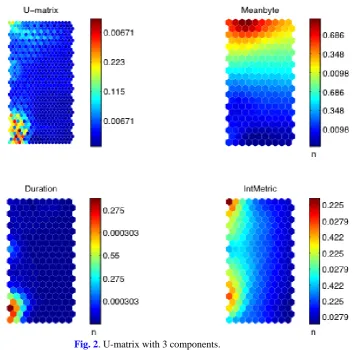
We use a unified distance matrix (U-matrix) to visualize the cluster structure of the map. From the U-matrix map, distances between neighboring map units can be visualized. This helps perceive how the clusters distribute in the map. High values of the U-matrix indicate a cluster border, whilst uniform areas of low values indicate clusters.
mean to standard deviation of interarrival times); total number of packets per connection; total number of bytes per connection; and root mean square of packet length.
Since the SOM algorithm uses the metric of Euclidean distance between vectors, the components of the data set must be normalized before any visualization. The common way to normalize is to linearly scale all variables, such that the variance of each variable becomes one, and the mean becomes zero. Typically, a Gaussian distribution is assumed for the variable, but we noticed that the Gaussian assumption was incorrect for the training data; the variables could not be normalized based on unit variance. Instead, we linearly scaled the value ranges of all the components to the range [0,1]; thus, none of the components could dominate the distance calculation.
[image:7.595.166.506.401.707.2]Fig. 1 shows the U-matrix and the components planes for the feature variables. The U-matrix is a visualization of distance between neurons, where distance is color coded according to the spectrum shown next to the map. Blue areas represent codebook vectors close to each other in input space, i.e., clusters. Red areas represent cluster separators, where codebook vectors are more separated in input space. Several observations we made from the map. First, there are at least three clusters in the map. Second, variable1, variable4, and variable7 are similar in shape. This indicates that the three features are highly linearly correlated. Third, variable5 and variable6 are highly linearly correlated. Fourth, there seems to be some correlation between variable3, variable5 and variable6.
We subsequently confirmed the linear correlation between feature components by plotting component-versus-component scatters. From the results, we chose to keep variable1, variable2 and variable3 as the most useful features. The remaining features were either correlated with another variable or not as important for clustering.
The U-matrix map was drawn using the reduced three feature variables. We noticed that some applications such as HTTP, SMTP, and FTP had a much larger number of connections than the other applications. We randomly selected equal samples from these applications to balance the
number of samples from all the applications to prevent data from these applications
dominating the map. The resulting U-matrix map is shown in Fig. 2. This map is a little
different, but resembles the previous map, still showing at least three clusters. Again, blue areas indicate clusters, whilst red areas indicate cluster separators. We applied the K-means
[image:8.595.157.515.312.662.2]clustering algorithm to the data set for further analysis.
Fig. 2. U-matrix with 3 components.
3.2 K-Means Clustering
The K-means clustering algorithm starts with a training data set and a given number of clusters
K. The samples in the training data set are assigned to a cluster based on a similarity
Er= xj−ci
2
j=1
n
∑
i=1
K
∑
(3) where K is the number of clusters and n is the number of training samples, ci is the center ofthe ith cluster, x−ci is the Euclidean distance between sample x and center ci of the ith
cluster.
We applied the K-means algorithm to segments from all four traffic traces with different
values of K, and ran the algorithm multiple times for each K. The best results were selected
based on the sum of squared errors. The Davies-Bouldin index was calculated for each
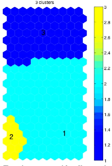
clustering. Fig. 3 shows the Davies-Boulding clustering index that is minimized with best
clustering. The Davies-Boulding index indicated that there are three clusters, consistent with the results from the self-organizing map.
After determining the presence of three clusters from both SOM and K-means clustering, we investigated the typical applications in each cluster. To check how different applications corresponded to the clusters in the data, we used so-called “hit” histograms in the self-organizing map. They are formed by taking a data set, finding the BMU of each data sample from the U-matrix map, and incrementing a counter in a map unit each time it is the BMU. The hit histogram shows the distribution of the data set on the map. From the hit histograms, it became evident that the three clusters were predominantly represented by four main applications: DNS in cluster 1, Telnet and FTP control in cluster 2, and HTTP in cluster 3.
We examined the features of packet length and connection duration of the applications to investigate the reference data set for the three classes. The mean and standard deviation of the features were plotted for individual applications. Inspection of the results suggested that the applications of interest could be clustered into three regions. The first region includes transactional applications, exemplified by DNS. The applications in this region have small average packet size and short connection duration time. The second region includes interactive applications, exemplified by Telnet and FTP control. Applications in this region have small average packet size, but long connection duration. The third region includes HTTP and represents the bulk transfer class. Applications have medium or large average packet size, but low or medium connection duration. Whilst our discovery of these three traffic classes is
consistent with the traffic classes proposed by Roughan et al. [6], we arrived at these traffic
classes by an unsupervised learning procedure, rather than making a priori assumptions. The
results of our procedure lend support to the intuitive arguments put forth in [6].
4. Experimental Classification Results
The previous section identified three clusters for QoS classes and features to build up classification rules through unsupervised learning. In this section, the accuracy of the classification rules is evaluated experimentally. For classification, we chose the K-nearest neighbor (KNN) algorithm. Experimental results are compared with the minimum mean distance (MMD) classifier.
classification, thus the importance of dimensionality is reduced.
Fig. 3. Three clusters suggested from K-means clustering.
In the KNN algorithm, we first calculate the Euclidean distance of a new data point Xi to all
the training data points Xi−Xj ( j=1,K ,K0), then the K nearest neighbors of Xi vote with
their class index C and the class Ci with highest proportion is assigned to data point Xi. In
some respect, the KNN approach can be viewed as an approximation to Bayesian classification.
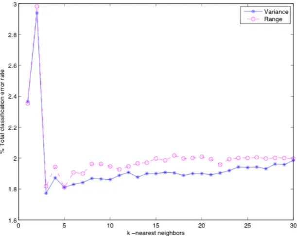
Since KNN uses the Euclidean metric to measure distances between vectors, the scaling of variables is important. Generally, the way to normalize data is to scale all variables so the variance of each variable equals one, but the underlying assumption is that the variables are Gaussian. Since the three feature variables we used in the classification are not Gaussian distributed, we compared variance normalization with range normalization, which scales all the variables to be within the range [0,1], by the classification error rates. Experimental results showed that the two normalization methods lead to similar accuracy. The variance normalization method has a slightly lower error rate than the range normalization method. Thus, variance normalization was used in the classifier.
The three feature vectors of the reference data set are shown in Fig. 4. The feature vectors
from different classes were significantly separated. We used the leave-one-out cross validation
method to test the validity of the classification algorithm. This method takes n training
[image:10.595.212.396.165.438.2]Fig. 4. Three feature vectors.
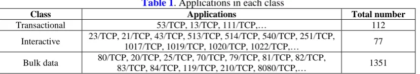
The three features used in the experiments were mean packet length per connection, connection duration, and interarrival variability, with three QoS classes: transactional, interactive, and bulk transfer. The 5NN algorithm was used for classification of all connections in the four traffic traces. Fig. 5, displays the classification error rates of the 5NN classifier for the two normalization methods. The selected application lists for each class and
the number of applications in each class are shown in Table 1.
[image:11.595.152.458.491.734.2]The accuracy of the 5NN classifier was compared to the minimum mean distance (MMD) classifier. The MMD classifier tries to condense information stored in the training data to a
reduced set of statistics, for example, the sample mean of the training data. For class wi, only
the sample mean μw
i of the training data belonging to the class is recorded. A test sample x is
classified to the class wi when μwi is closest to it. However, since the μwi does not contain
the information about the spatial distribution of training samples, but covariance matrix Σi
does, we use the normalized distance, (x−μw
i)
TΣ i
−1
(x−μw
i) , to measure the distance
[image:12.595.100.515.293.366.2]between samples and cluster means. The misclassification rate for the MMD classifier was found to be 7.26%, significantly worse than the 5NN classifier.
Table 1. Applications in each class
Class Applications Total number
Transactional 53/TCP, 13/TCP, 111/TCP,… 112
Interactive 23/TCP, 21/TCP, 43/TCP, 513/TCP, 514/TCP, 540/TCP, 251/TCP,
1017/TCP, 1019/TCP, 1020/TCP, 1022/TCP,… 77
Bulk data 80/TCP, 20/TCP, 25/TCP, 70/TCP, 79/TCP, 81/TCP, 82/TCP,
83/TCP, 84/TCP, 119/TCP, 210/TCP, 8080/TCP,… 1351
5. Conclusions
Traffic classification was carried out in two phases. In the first off-line phase, we started with no assumptions about traffic classes and used the unsupervised SOM and K-means clustering algorithms to find the structure in the traffic data. The data exploration procedure found three clusters corresponding to three QoS classes: transactional, interactive, and bulk data transfer. This result lends experimental support to previous arguments for a similar set of traffic classes. In addition, we found that the three most useful features among the candidate features were mean packet length, connection duration, and interarrival variability. This is not to say that the
discovered set of traffic classes is optimal in any sense. The composition of Internet traffic is constantly changing due to new applications and fluctuations in the popularity of different
applications over time. It is necessary to continually re-examine traffic. This is likely to uncover new traffic classes.
In the second classification phase, the accuracy of the KNN classifier was evaluated for test data. Leave-one-out cross-validation tests showed that this algorithm had a low error rate. The KNN classifier was found to have an error rate of about 2 percent for the test data, compared to
an error rate of 7 percent for a MMD classifier. KNN is one of the simplest classification algorithms, but not necessarily the most accurate. Other supervised algorithms, such as back
propagation (BP) and SVM, also have attractive features and should be compared in future work.
References
[1] Thuy Nguyen and Grenville Armitage, “A survey of techniques for Internet traffic classification using machine learning,” IEEE Communications Surveys and Tutorials, vo.10, no.4, pp.56-76, 2008.
[2] H. Trussell, A. Nilsson, P. Patel, and Y. Wang, “Estimation and detection of network traffic,” in
Proc. of 11th Digital Signal Processing Workshop, pp.246-248, 2004.
machine learning techniques,” in Proc. of 5th Int. Workshop on Passive and Active Network Measurement, pp.205-214, 2004.
[4] Sebastian Zander, Thuy Nguyen, and Grenville Armitage, “Self-learning IP traffic classification based on statistical flow characteristics,” in Proc. of 6th Int. Workshop on Passive and Active Measurement, pp.325-328, 2005.
[5] Sebastian Zander, Thuy Nguyen, and Grenville Armitage, “Automated traffic classification and application identification using machine learning,” in Proc. of IEEE Conf. on Local Computer Networks, pp.250-257, 2005.
[6] Matthew Roughan, Subrabrata Sen, Oliver Spatscheck, and Nick Duffield, “Class-of-service mapping for QoS: a statistical signature-based approach to IP traffic classification,” in Proc. of 4th ACM SigComm Conf. on Internet Measurement, pp.135-148, 2004.
[7] Andrew Moore and Dennis Zuev, “Internet traffic classification using Bayesian analysis techniques,” in Proc. of ACM Sigmetrics Int. Conf. on Measurement and Modeling of Computer Systems, pp.50-60, 2005.
[8] Tom Auld, Andrew Moore, and Stephen Gull, “Bayesian neural networks for Internet traffic classification,” IEEE Trans. on Neural Networks, vol.18, no.1, pp.223-239, Jan. 2007
[9] Thomas Karagiannis, Konstantina Papagiannaki, and Michalis Faloutsos, “BLINC: multilevel traffic classification in the dark,” ACM Sigcomm Computer Communications Review, vol.35, no.10, pp.229-240, 2005.
[10]Laurent Bernaille, Renata Teixeira, Ismael Akodkenou, Augustin Soule, and Kave Salamatian, “Traffic classification on the fly,” ACM Sigcomm Computer Communications Review, vol.36, no.4, pp.23-26, Apr. 2006.
[11]Nigel Williams, Sebastian Zander, and Grenville Armitage, “A preliminary performance comparison of five machine learning algorithms for practical IP traffic flow classification,” ACM Sigcomm Computer Communications Review, vol.36, no.10, pp.5-16, Oct. 2006.
[12]Jeffrey Erman, Martin Arlitt, and Anirban Mahanti, “Traffic classification using clustering algorithms,” in Proc. of ACM Sigcomm Workshop on Mining Network Data, pp.281-286, 2006. [13]Jeffrey Erman, Anirban Mahanti, Martin Arlitt, and Carey Williamson, “Identifying and
discriminating between web and peer-to-peer traffic in the network core,” in Proc. of 16th Int. Conf. on World Wide Web, pp.883-892, 2007.
[14]Liu Yingqiu, Li Wei, and Li Yunchun, “Network traffic classification using k-means clustering,” in Proc. of 2nd Int. Multisymposium on Computer and Computational Sciences, pp.360-365, 2007 [15]Manuel Crotti, Francesco Gringoli, Paolo Pelosato, and Luca Salgarelli, “A statistical approach to
IP-level classification of network traffic,” in Proc. of IEEE ICC 2006, pp.170-176, 2006.
[16]Manuel Crotti, Maurizio Dusi, Francesco Gringoli, and Luca Salgarelli, “Traffic classification through simple statistical fingerprinting,” ACM Sigcomm Computer Communications Review, vol.37, no.1, pp.7-16, Jan. 2007.
[17]Hajime Inoue, Dana Jansens, Abdulrahman Hijazi, and Anil Somayaji, “NetADHICT: a tool for understanding network traffic,” in Proc. of Usenix Large Installation System Administration Conf., pp. 39-47, 2007.
[18]Jin Cao, Aiyou Chen, Indra Widjaja, and Nengfeng Zhou, “Online identification of applications using statistical behavior analysis,” in Proc. of IEEE Globecom 2008, pp.1-6, 2008.
[19]Charles Wright, Fabian Monrose, and Gerald Masson, “On inferring application protocol behaviors in encrypted network traffic,” J. of Machine Learning Research, vol.7, no.12, pp.2745-2769, Dec. 2006.
[20]Alberto Dainotti, Walter de Donato, Antonio Pescape, and Pierluigi Salvo Rossi, “Classification of network traffic via packet-level hidden Markov models,” in Proc. of IEEE Globecom 2008, pp.1-5, 2008.
Yi Zeng received a B.S. degree from Harbin Institute of Technology, China, in 1994, a M.S. degree from Nanjing University of Posts and Telecommunications, China in 1999, and a Ph.D. degree from Southern Methodist University, Dallas, Texas, in 2008. She is currently with the San Diego Supercomputer Center in the University of California, San Diego. Her research interests include Internet data mining, data classification, statistical modeling the Internet traffic, network self-similarity, and machine learning.
Thomas M. Chen is a Professor in Networks at Swansea University in Swansea, Wales, UK. He received BS and MS degrees in electrical engineering from the Massachusetts Institute of Technology, and PhD in electrical engineering from the University of California, Berkeley, USA. He worked at GTE Laboratories (now Verizon) in Waltham, Massachusetts, and then the Department of Electrical Engineering at Southern Methodist University, Dallas, Texas, as an associate professor. He joined Swansea University in May 2008. He is the co-author of ATM Switching (Artech House) and co-editor of Broadband Mobile Multimedia: Techniques and Applications (CRC Press). He is currently editor-in-chief of IEEE Network and was former editor-in-chief of
![Fig. 1. U-matrix with 7 components scaled to [0,1].](https://thumb-us.123doks.com/thumbv2/123dok_us/1618058.114848/7.595.166.506.401.707/fig-u-matrix-components-scaled.webp)