Turing instability in discrete replicator systems

(1)

Rochester Institute of Technology

RIT Scholar Works

Theses Thesis/Dissertation Collections

4-15-2011

Turing instability in discrete replicator systems

Alex Bryce

Follow this and additional works at:http://scholarworks.rit.edu/theses

Recommended Citation

(2)

Turing Instability in Discrete Replicator Systems

by

Alex J. Bryce

Submitted to the School of Mathematical Sciences

in partial fulfillment of the requirements for the degree of

Masters of Science in Applied & Computational Mathematics

at the

ROCHESTER INSTITUTE OF TECHNOLOGY

April 2011

c

Author . . . .

School of Mathematical Sciences

April 15, 2011

Certified by . . . .

Bernard P. Brooks

Associate Professor

Thesis Supervisor

(3)

Turing Instability in Discrete Replicator Systems

by

Alex J. Bryce

Submitted to the School of Mathematical Sciences on April 15, 2011, in partial fulfillment of the

requirements for the degree of

Masters of Science in Applied & Computational Mathematics

Abstract

When analyzing a discrete reaction-diffusion dynamical system, one primary area of interest is locating where in the parameter space Turing instabilities occur. It will be shown that Turing instabilities cannot occur in the react then diffuse equations if all diffusion coefficients are equal. The replicator dynamic is a system of equations that is used in evolutionary game theory applications to study behavior types in animal populations. Conditions for a Turing instability in first order discrete replicator systems will be discussed and illustrated with computer simulations of the results.

(4)

Acknowledgments

First and foremost, I’d like to offer my gratitude to my advisor, Dr. Bernard P.

Brooks for his consistent patience and support as I worked to complete the thesis

while juggling classes, teaching, tutoring, and searching for a job simultaneously. I’d

also like to thank Dr. Michael Radin and Dr. Tamas Wiandt for serving on my

committee. Their questions and comments forced me to think about ways to write

my thesis in order to make it understandable by other readers. Finally, I’d also like

to give special thanks to all of the great math interpreters I’ve had the pleasure to

work with at RIT, especially Deborah Makowski who interpreted my meetings with

Dr. Brooks for the entire year.

Next, I’d like to thank Dr. Jonathan Forde. My passion for dynamical systems

and mathematical biology both stem from the two courses and an independent study

I took with him as an undergraduate at Hobart and William Smith Colleges. His

enthusiasm for these two subjects sparked my own interest, and inspired me to explore

these subjects at RIT. Now that I’m about to receive my graduate degree in applied

mathematics, my next goal is to get a doctorate in mathematical biology.

Last, but not the least, I’d like to thank my family and friends. Their patience,

(5)

List of Figures

2-1 Example of replicator dynamic favoring a Retaliator-Dove distribution 10

2-2 Example of replicator dynamic favoring a Retaliator-only distribution 11

2-3 Example of replicator dynamic favoring a Hawk-Bully distribution . . 12

3-1 Visual example of Turing instability . . . 24

4-1 Graph of the Dove population with and without diffusion . . . 39

(8)

Chapter 1

Introduction

The replicator dynamic has applications in evolutionary game theory, particularly

in the analysis of animal behavior. Dawkins defined replicators as entities which

can make (in theory) an infinite number of perfect copies of themselves, but their

inherent properties can affect their chances of being copied [4]. Hence, sexually

reproducing individuals such as human beings are not replicators (since their children

are not perfect copies of themselves). However, their genes can be considered to be

replicators since genes can be passed on from parent to child indefinitely with an

inherent chance of being mutated or not inherited.

For the purposes of this paper, we will focus specifically on behavior types that are

passed on from a parent to child within a population of a single generic animal species.

Beginning with the discrete replicator dynamic, which describes the changes in the

frequency of behavior types over time, we incorporate diffusion into the dynamical

system and analyze it for instances of Turing instability.

The paper is divided into two parts. The first half will focus on establishing

(9)

into a discrete dynamical system. In the second chapter, we will give a formal

mathematical definition for the replicator dynamic. In addition, we will establish the

framework for applying the replicator system to study the interactions of different

behavior tendencies within a population of a single animal species. We also provide

4-dimensional examples. In the third chapter, we will discuss discrete diffusion and

temporal and spatial stability, and then we will define Turing instability. We will

also construct a general linearized system of equations incorporating diffusion from

which we will derive a Jacobian matrix for analyzing the linear spatial stability of

equilibrium points of the system.

The second half of the paper will focus on analyzing the replicator system for

instances of Turing instability. In the fourth chapter, we will prove that the Jacobian

of a replicator system always has a zero determinant. Next, we will prove that it is

impossible to cause Turing instability in the two-dimensional replicator system. We

will also discuss the possibilities of Turing instability in the three-dimensional and

four-dimensional replicator systems. In the fifth chapter, we will consider a similar

problem of using diffusion to turn unstable equilibrium points into stable equilibrium

(10)

Chapter 2

The Discrete Replicator Dynamic

2.1

Defining the Replicator Dynamic

Consider a population consisting of a single animal species with n behavior

tenden-cies. Letxi(t) be the frequency of typei behavior tendency at discrete time t. Each

of these behavior types is considered to be a replicator and we will analyze the

fit-ness of these behaviors in interaction with each other as individuals compete over a

needed resource for survival and propagation of the species (such as food or potential

mates). Assume that xi(t) are differentiable functions of time t and that the state

of the population at time t is given by the vector ~x which is an element of the unit

simplex. That is,

n X

i=1

xi(t) = 1

0≤xi(t)≤1

We allow random encounters between individuals. The outcome of these encounters

(11)

change in fitness, defined as the number of offspring produced, for the ith _{type after}

an encounter with the jth type [8]. We assume without loss of generality that A is

a nonnegative square matrix of size n, which is supported by the interpretation of

the interactions: if the ith behavior type individual wins an encounter against the

jth _{behavior type individual, then it is able to produce offspring. However, if the}

ith behavior type individual loses the encounter, then it is not able to survive and

produce offspring. (A~x)i is the expected payoff for the type i individual and ~xTA~x

is the average payoff for the entire population [5].

We define the general discrete replicator equation as

xi(t+ 1) =xi(t)

(A~x)i

~ xT_A_~_x

(2.1)

The fraction (A~x)i

~

xT_A_~_x compares the fitness of theith type with the entire population. If

the expected payoff for the ith _{population is greater than the average payoff, then}

the ratio becomes greater than 1 and the ith _{population grows. Conversely, if the}

expected payoff is smaller than the average payoff, then the ratio is smaller than 1

and the ith _{population shrinks. Since} _x

i(t) represent population frequencies, they

are dimensionless variables. In addition, both the numerator and the denominator

of the fraction have the same units (the number of offspring produced) which cancels

out. Therefore, the replicator equation is dimensionless.

Since we have n different behavior tendencies, the replicator system is a system

of n replicator equations of the form 2.1. Since we are working with a system of

difference equations, the equilibrium points are the points such that

~

(12)

Note that for any arbitrary i, we have

xi(t) =xi(t)

(A~x)i

~ xT_A_~_x

0 =xi(t)

(A~x)i

~

xT_A_~_x −xi(t)

0 =xi(t)

(A~x)i

~

xT_A_~_x −1

Since the xi are constrained on the unit simplex, we ignore the trivial solution:

xi(t) = 0 for all i. Note that we can reduce the dimension of the problem by forcing

at least one xi to be zero. If xi 6= 0 for all i, then the equilibrium point is in the

interior of the simplex and is the solutions to the following system of linear equations:

(A~x)1 = (A~x)2 =...= (A~x)n n

X

i=1

xi(t) = 1

As an application of this system, consider a single animal species competing with

itself for a food resource. All individuals, upon encountering another individual,

can either “display,” a method of displaying aggressiveness to scare individuals off

without fighting, or “escalate,” creating a physical conflict. Within this single species

are four behavior tendencies that affect the way an individual interact with another

individual when competing over the resource. “Hawks” will always escalate until

the opponent flees or either one of them is injured. “Doves” will always display but

retreat if the opponent escalates. “Retaliators” will escalate a conflict only if the

opponent escalates first. “Bullies” will escalate conflicts, but always retreat if the

opponent escalates as well [4].

(13)

opponent and winning the resource and 50% chance of being injured. Assume also

that two displaying opponents both have a 50% chance of winning the resource. Let

Gbe the gain in the fitness from winning an encounter and C to be the decrease in

fitness from sustaining injuries [1]. We will assume also that 0 < G < C [8]. This

makes sense as conflict creates a risk of being killed for the combatants (as the loser

will be killed or injured during combat, unable to produce offspring). Then we can

devise a system of 4 replicator equations with the following fitness matrix:

Hawk Dove Retaliator Bully

Hawk G−₂C G G−₂C G

Dove 0 G₂ G₂ 0

Retaliator G−₂C G₂ G₂ G

Bully 0 G 0 0

A=        

G−C

2 G

G−C

2 G

0 G₂ G₂ 0

G−C

2

G

2

G

2 G

0 G 0 0

       

Since G−₂C <0 and A must be nonnegative, we shift A by adding C−₂G to every entry, giving us the new matrix

A=        

0 C+G

2 0

C+G

2

C−G

2

C

2

C

2

C−G

2

0 C

2

C

2

C+G

2

C−G

2

C+G

2

C−G

2

C−G

(14)

This shift has no effect on the behavior of the replicator equation, and so it will not

affect the location or the behavior of our equilibrium points [5].

As a simplification of the problem, we proceed to eliminate the parameter G.

Since 0< G < C , let G=mC where 0< m < 1. Making the substitution into the

matrix allows us to eliminateG entirely.

A=        

0 C+₂mC 0 C+₂mC

C−mC

2

C

2

C

2

C−mC

2

0 C₂ C₂ C+₂mC

C−mC

2

C+mC

2

C−mC

2

C−mC

2        

A nice feature of this substitution is that everything is written in terms of C,

which can be factored out of the matrix as shown:

A= C

2        

0 1 +m 0 1 +m

1−m 1 1 1−m

0 1 1 1 +m

1−m 1 +m 1−m 1−m

       

A= C

2A1

(15)

scalar. We then are able to cancel outC from the replicator equation as follows:

xi(t+ 1) =xi(t)

(A~x)i

~xT_A_~_x

xi(t+ 1) =xi(t)

(C₂A1~x)i

~xT C

2A1~x

!

xi(t+ 1) =xi(t) C

2(A1~x)i

C

2~xTA1~x

!

xi(t+ 1) =xi(t)

(A1~x)i

~xT_A

1~x

Thus, instead of analyzing the replicator system that contains two parametersC and

G, we can analyze the equivalent system that has only one dimensionless parameter

m∈(0,1).

2.2

Equilibirum Points for the Replicator Dynamic

In the two dimensional case (population consists of only Hawks and Doves.), the

equilibrium points are as follows:

(H, D)∈ {(1,0),(0,1),(m,1−m)}

In the three-dimensional case (population consists of only Hawks, Doves, and

Retal-iators), the equilibrium points are as follows:

(16)

where 0< α <1. In the four-dimensional case (all behavior types are represented),

the equilibrium points are as follows:

(H, D, R, B)∈

(0,0,0,1),(0,0,1,0),(0,1,0,0),(1,0,0,0),(m,1−m,0,0),

(0, α,1−α,0),

2m

1 +m,0,0,

1−m

1 +m

where 0 < α < 1. The eigenvalues of the Jacobian evaluated at each equilibrium

point for each case will be discussed in their respective sections in Chapter 4.

2.3

Replicator Dynamic Examples

As an example, let’s investigate how the four-dimensional dynamic behaves if we set

m= 2/3 and consider different initial population distributions.

Suppose we start with an initial population distribution that is equally divided

among four behavior tendencies: ~x = (0.25,0.25,0.25,0.25). Then as time goes

by, the interaction between the four behavior types causes the Hawk and the Bully

behavior tendencies to become extinct and the population is composed of 80%

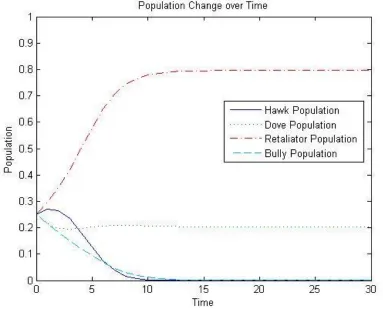
Re-taliators and 20% Doves as shown in Figure 2-1. This corresponds to the equilibirum

point (0, α,1−α,0) where α= 0.2.

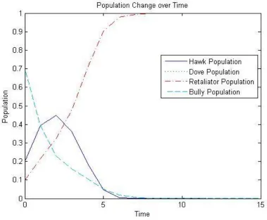
Suppose we start with the initial population distribution ~x = (0.2,0,0.1,0.7).

Then the dynamic will flow toward a population consisting of only Retaliators as

shown in Figure 2-2. This corresponds to the equilibirum point (0,0,1,0).

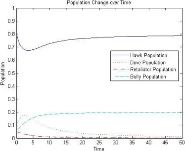
Finally, suppose we start with the initial population distribution

~x = (0.8,0.1,0.05,0.05). Then the dynamic will flow toward an equilibrium point

consisting of 80% Hawks and 20% Bullies as shown in Figure 2-3. This corresponds

(17)

[image:17.612.112.495.104.413.2]

Figure 2-1: Graph showing how the replicator dynamic favors a Retaliator-Dove distribution if we start with equal amounts of all behavior tendencies.

These three figures all show how the replicator dynamic behaves over time for

different initial population distributions. Note that we assumed that the entire

pop-ulation resides in a single community where any individual could interact with any

other individual. In the next chapter, we will introduce a spatial dimension into the

dynamical system, to emulate the concept that individuals may be restricted in whom

they are able to interact with because the popluation is distributed among different

(18)

[image:18.612.113.492.102.415.2]

Figure 2-2: Graph showing how using a different initial population distribution causes the replicator dynamic to favor a Retaliator-only distribution.

(19)

[image:19.612.115.489.192.498.2]

(20)

Chapter 3

Incorporating Diffusion into the

Discrete Dynamical System

3.1

Discussing Discrete Diffusion

When we incorporate diffusion into our dynamical system, we introduce a spatial

dimension into our analysis, so that our population dynamic can change through

space as well as time. For simpler analysis, we will restrict diffusion to one dimension,

so that the population can only move in two directions (i.e., to the left or to the right).

We define our spatial region as a ring of k cells, setting cell 0 and cell k to be

the same cell. Let xs

i(t) be the ith population in cell s at time t. Then for any s

such that 1≤s ≤k, populations in cells can only diffuse with cellss−1 ands+ 1.

This allows us to avoid dealing with boundary conditions (or to incorporate periodic

boundary conditions). With k cells, we now have a system of nk equations.

For each variablexi(t), there is an associated diffusion constant,di ∈[0,0.5]. The

(21)

of the population within a cell and its adjacent cells. If we have a full cell and two

adjacent cells that are both empty, then we can move up to half of the population

from the full cell to each of the empty cells. Hence, the diffusion constant is capped

at 0.5.

The ring system has an useful property. Suppose a dynamical system has the

equilibrium point (a1, a2, . . . , an). When we introduce the ring of spatial cells, we

treat each cell as an independent and identical dynamical system, and (a1, a2, . . . , an)

is also an equilibrium point for each cell. The ring system then has a ”global”

equilibrium point wherexs

i =ai for all cellss, 1≤s≤k [7].

For example, the Hawk-Dove dynamic has (m,1−m) as an equilibrium point. If

we construct a 3-cell ring system for this dynamic, then each cell can be treated as

its own dynamical system that also has (m,1−m) as an equilibrium point. However,

since we must also adhere to the restriction that all population frequencies add up

to 1, we have to scale the equilibrium point in each cell. Therefore, the global

equilibrium point isxs

1 =

m

3 and x

s

2 = 1−m

3 for 1≤s≤3.

The introduction of diffusion into the dynamical system transforms it from a

purely reaction dynamic (where population values changed over time through

in-teraction with other populations) to a reaction-diffusion dynamic. Now population

frequencies will be affected by both the interaction with other population frequencies

and the spatial motion from one cell to another cell.

In a purely reaction dynamic, the stability of an equilibrium point is purely

temporal; either the initial point near the equilibrium point moves away from or

closer to the equilibrium point as time progresses. When the spatial dimension is

added and the reaction dynamic becomes a reaction-diffusion dynamic, we have to

concern ourselves with whether population values in the spatial cells will remain the

(22)

we discuss stability for the reaction-diffusion dynamic, we have to consider both

temporal and spatial stability.

An equilibrium point will be linearly temporally stable if all eigenvalues of the

Jacobian of the reaction dynamic evaluated at this point have magnitude less than

1. When this occurs, then any initial point near the temporally-stable equilibrium

point will move toward it as time passes. If there is at least one eigenvalue that has

a magnitude greater than 1, then the equilibrium point will be temporally-unstable

and any initial point near the equilibrium point will move away from it as time goes

by. If the equilibrium point has at least one eigenvalue equal to 1, then the linear

stability test is inconclusive; it may or may not be stable.

An equilibrium point will be linearly spatially stable if, after the ring system and

diffusion is incorporated into the reaction dynamical system, all eigenvalues of the

Jacobian of the reaction-diffusion dynamic evaluated at this point have magnitude

less than 1 for all cells in the system. If there is at least one cell with at least

one eigenvalue with a magnitude greater than 1, then the equilibrium point will be

spatially unstable. If the equilibrium point has at least one eigenvalue equal to 1 in

any cell, then the linear stability test is inconclusive; it may or may not be stable.

Turing instability occurs when a temporally-stable equilibrium point becomes

spatially-unstable after diffusion is introduced into the system [5, 7].

As a visual example of a Turing instability, consider the two graphs shown in

Figure 3.1, both of which represents the same Dove population, one without diffusion

and one with diffusion. In Figure 3-1(a), no diffusion is introduced into the system.

Notice that the spatial distribution of the population becomes constant over time.

Figure 3-1(b) shows what happens when we introduce diffusion into the system.

Notice that the population distribution over the cells are constantly changing. This

(23)

finding.

The focus of this paper will be to analyze where in parameter space Turing

in-stability occurs in replicator systems. To do so, we need to figure out a way to

incorporate diffusion into the dynamical system. Discrete diffusion is more

problem-atic than continuous diffusion. In continuous diffusion, the diffusionable material

is able to react with itself and diffuse simultaneously. However, when dealing with

discrete diffusion, we have to choose whether to react first then diffuse or to diffuse

first then react. In the continuous case, it is impossible to achieve Turing instability

if all diffusion coefficients are the same [2]. It will be shown that a similar result

occurs for the discrete reaction-diffusion system, making it a better choice over the

discrete diffusion-reaction system.

3.2

Constructing the Reaction-Diffusion System

Consider a linearized system of 2 discrete differential equations. Subdivide the spatial

region into k cells. Incorporating one-dimensional diffusion into the system

(empha-sizing that reaction occurs before diffusion) gives us the following system





xs₍_t_{+ 1)}

ys(t+ 1)



=J· 



xs₍_t₎

ys(t)



+ 



dx 0

0 dy 

 

J· 



xs−1₍_t₎

ys−1(t)





−2J· 



xs₍_t₎

ys(t)



+J· 



xs+1₍_t₎

ys+1(t)



 



where J denotes the Jacobian evaluated at the equilibrium point and dx and dy are

(24)

When we explicitly write out each equation, we obtain 2k equations of the form

xs(t+ 1) =J11xs(t) +J12ys(t)

+dxJ11 xs−1(t)−2xs(t) +xs+1(t)

+dxJ12 ys−1(t)−2ys(t) +ys+1(t)

ys(t+ 1) =J21xs(t) +J22ys(t)

+dyJ21 xs−1(t)−2xs(t) +xs+1(t)

+dxJ22 ys−1(t)−2ys(t) +ys+1(t)

Notice that both equations depends on the s−1, s, and s + 1 cells. In order to

investigate linear stability of the coexistence equilibrium in the presence of diffusion,

we will decouple the 2k equations by transforming the x and y variables into u and

v variables. Define the discrete Fourier transform as

xr(t) =

k−1

X

r=0

e2irsπk ur(t)→ur(t) = 1 k

k X

s=0

e−2irsπk xs(t)

yr(t) =

k−1

X

r=0

e2irsπk vr(t)→vr(t) = 1 k

k X

s=0

e−2irsπk ys(t)

This decoupling transformation will also transform the spatial dimension for easier

analysis, so that equations will depend only on cell r instead of cells s−1, s, and

(25)

Performing the transformation on the first equation:

ur(t) = 1

k

k X

s=1

e−2irsπk xs(t)

= 1

k

k X

s=1

e−2irsπk J₁₁xs(t) +J₁₂ys(t) +d_xJ₁₁ xs−1(t)−2xs(t) +xs+1(t)

+dyJ12 ys−1(t)−2ys(t) +ys+1(t)

=J11

1

k

k X

s=1

e−2irsπk xs(t) +J

12 1 k k X s=1

e−2irsπk ys(t)

+dxJ11

1

k

k X

s=1

e−2irsπk xs−1(t)− 2 k

k X

s=1

e−2irsπk xs(t) + 1 k

k X

s=1

e−2irsπk xs+1(t)

!

+dxJ12

1

k

k X

s=1

e−2irsπk ys−1(t)− 2 k

k X

s=1

e−2irsπk ys(t) + 1 k

k X

s=1

e−2irsπk ys+1(t)

!

=J11

1

k

k X

s=1

e−2irsπk xs(t) +J₁₂1 k

k X

s=1

e−2irsπk ys(t)

+dxJ11

1

ke

−2irπ k

k X

s=1

e−2ir(ks−1)πxs−1(t)− 2 k

k X

s=1

e−2irsπk xs(t)

+1 ke 2irπ k k X s=1

e−2ir(ks+1)πxs+1(t)

!

+dxJ12

1

ke

−2irsπ k

k X

s=1

e−2ir(ks−1)πys−1(t)

−2

k

k X

s=1

e−2irsπk ys(t) + 1 ke 2irπ k k X s=1

e−2ir(ks+1)πys+1(t)

!

Using the fact that if 0< r < k, then

k X

s=1

(26)

and if r= 0 or r=k, then

k X

s=1

e2irsπk =k

we simpify the equation to obtain

ur(t+ 1) =J11ur(t) +J12vr(t) +dxJ11

e−2kirπ −2 +e

2irπ k

ur(t)

+dxJ12

e−2kirπ −2 +e

2irπ k

vr(t)

Using Euler’s formula and trignometric properties, we hide the imaginary terms to

get:

ur(t+ 1) =J11ur(t) +J12vr(t)−4dxJ11sin2

rπ

k

ur(t)−4dxJ12sin2

rπ

k

vr(t)

=J11

1−4dxsin2 rπ

k

ur(t) +J12

1−4dxsin2 rπ

k

vr(t)

The second equation is transformed similiarly, and we obtain a transformed

sys-tem of equations:

ur(t+ 1) =J11

1−4dxsin2 rπ

k

ur(t) +J12

1−4dxsin2 rπ

k

vr(t)

vr(t+ 1) =J21

1−4dysin2 rπ

k

ur(t) +J22

1−4dysin2 rπ

k

vr(t)

We can rewrite this linearized system of equations in the following matrix form:





ur₍_t_{+ 1)}

vr₍_t_{+ 1)} 

= 



1−4dxsin2 rπ_k

0

0 1−4dysin2 rπ_k



J 



ur₍_t₎

vr₍_t₎ 



This matrix system of equations represents a linearized two-dimensional discrete

(27)

to any two-dimensional discrete dynamical system in which we wish to search for

Turing instability.

We follow this same procedure for an n-dimensional discrete dynamical system

with k cells. After incorporating diffusion into a linearized n-dimensional system,

the population vector for cell s, −−→xs₍_t_{), 1}_≤_s_≤_k _{at any given time}_t _{is given by}

−−−−−→

xs(t+ 1) =J−−→xs(t) +DJ−−−−→xs−1(t)−2J−−→xs(t) +J−−−−→xs+1(t)

where J denotes the Jacobian of the discrete dynamical system evaluated at the

equilibrium point and D is a diagonal matrix of diffusion constants.

Explictly writing out the equations results in

xs₁(t+ 1) =

n X

j=1

J1jxsj(t) + n X

j=1

d1J1j xsj−1(t)−2x s

j(t) +x s+1

j (t)

xs₂(t+ 1) =

n X

j=1

J2jxsj(t) + n X

j=1

d2J2j xsj−1(t)−2x s

j(t) +x s+1

j (t)

.. .

xs_n(t+ 1) =

n X

j=1

Jnjxsj(t) + n X

j=1

dnJnj xsj−1(t)−2x s

j(t) +x s+1

j (t)

By using the same transformation as presented in the two-dimensional case, we can

(28)

equations:

ur₁(t+ 1) =

n X

j=1

J1j

1−4d1sin

rπ

k

ur_j(t)

ur₂(t+ 1) =

n X

j=1

J2j

1−4d2sin

rπ

k

ur_j(t)

.. .

ur_n(t+ 1) =

n X

j=1

Jnj

1−4dnsin rπ

k

ur_j(t)

which we can rewrite into the following matrix form:



   

ur₁(t+ 1) .. .

ur_n(t+ 1)

     =     

1−4dxsin2 rπ_k

· · · 0

..

. . .. ...

0 · · · 1−4dnsin2 rπ_k      J     

ur₁(t) .. .

ur_n(t)

     (3.1)

Note thatJ is the Jacobian of some given dynamical system. Thus, the given matrix

system is a general linearizedn-dimensional reaction-diffusion dynamical system that

can be applied to any discrete n-dimensional dynamical system in order to search

for Turing instability.

The Jacobian of (3.1), which we denote as Γ, is defined as

Γ =     

1−4d1sin2 rπ_k

· · · 0

..

. . .. ...

(29)

where the trace and the determinant of (3.2) are given as follows:

tr(Γ) =tr(J)−4 sin2rπ

k

_Xn

i=1

Jiidi (3.3)

det(Γ) =det(J)

n Y

i=1

1−4disin2 rπ

k

(3.4)

We can use (3.2) to analyze the stability of equilbirum points of any discrete

dy-namical system in the presence of diffusion and determine where Turing instabilities

occur.

To ensure that our discrete reaction-diffusion dynamical system corresponds with

the continuous reaction-diffusion dynamical system, we need to show that Turing

instability will not occur if all diffusion coefficients are equal.

Theorem 1. Turing instabilities cannot occur in a n-dimensional discrete

reaction-diffusion dynamical system with one-dimensional reaction-diffusion if all reaction-diffusion coefficients

are equal.

Proof. Consider an-dimensional discrete dynamical system with an temporally

sta-ble equilbirum point. Let J be the Jacobian of the dynamical system evaluated at

the temporally stable equilibrium point. Let 1-dimensional diffusion be incorporated

into the system so it becomes the transformed reaction-diffusion dynamical system

given in (3.1).

The Jacobian of (3.1) is given by (3.2). Assume that all diffusion coefficients are

equal. That is,

0≤d1 =d2 =· · ·=dn≤0.5

(30)

and a scalar:

Γ =

1−4d1sin2

rπ

k

J

Suppose there is no diffusion, implying that d1 = 0. Then Γ = J. Since the

equilbirum point is temporally stable by assumption, all eigenvalues of the Jacobian

J have magnitude less than 1, and therefore Γ is also stable.

Suppose we maximize diffusion, implying thatd1 = 0.5. Then the scalar becomes

1−2 sin2 rπ_k . Since 1≤r≤k, 1−2 sin2 rπ_k ∈[−1,1]. SinceJis evaluated at the temporally-stable equilibrium point, then all of its eigenvalues have magnitude

less than 1. Multiplying J by the scalar shrinks these eigenvalues so the eigenvalues

of Γ are guaranteed to have magnitude less than 1. Therefore, the equilibrium point

is spatially stable.

Since the temporally-stable equilibrium point is spatially stable for any diffusion

constant, Turing instability cannot occur if all diffusion constants are equal.

Thus, our linearized discrete reaction-diffusion dynamical system corresponds to

the continuous reaction-diffusion case, and we can apply this system to the replicator

(31)

(a)

[image:31.612.161.441.99.593.2]

(b)

(32)

Chapter 4

Searching for Turing Instability in

Discrete Replicator Systems

4.1

Turing Instability in Replicator Dynamics

Now that we have constructed the general reaction-diffusion dynamical system with

one-dimensional diffusion, we can begin to analyze replicator dynamics for presence

of Turing instability. First, it is useful to prove one fact about the Jacobian of the

replicator system.

Theorem 2. The determinant of the Jacobian of any n-dimensional replicator

sys-tem is 0.

Proof. Consider an-dimensional replicator system. The variablexi(t) represents the

population frequency of the ith _{type in the population at time} _t_{. By assumption,}

n X

i=1

(33)

Hence, without loss of generality, we see that

xn(t) = 1− n−1

X

i=1

xi(t)

xn(t) = 1−x1(t)−x2(t)−...−xn−1(t)

x0_n(t) =−x0₁(t)−x0₂(t)−...−x0_n₋₁(t)

wherexi(t) is the replicator equation for the variablexi and 0 represents the partial

derivative.

Consider the Jacobian of the replicator system.

J=     

∂x1(t)

∂x1 . . .

∂x1(t)

∂xn

..

. . .. ...

∂xn(t)

∂x1 . . .

∂xn(t)

∂xn     

For any arbitrary column j, ∂xn(t)

∂xj can be expressed as a linear combination of the

other column entries. That is, for all j, 1≤j ≤n,

∂xn(t)

∂xj

=−

n−1

X

i=1

∂xi(t)

∂xj

Thus, the nth _{row can be expressed as a linear combination of the other rows.}

Therefore, det(J) = 0.

This fact indicates that for any n-dimensional replicator system, all equilibrium

(34)

4.2

Turing Instability in the Two-Dimensional Case

Using the fact that the determinant of the Jacobian is always zero, we can prove

that Turing instability cannot occur in the two-dimensional case.

Theorem 3. Turing instability cannot occur in the two-dimensional case.

Proof. Consider the general two-dimensional discrete replicator system with

non-overlapping generations where x1(t) and x2(t) are nonnegative for all t. Such a

system has the following form:

x1(t+ 1) =x1(t)

(A~x)1

~ xT_A_~_x

x2(t+ 1) =x2(t)

(A~x)2

~ xT_A_~_x

where A is a general nonnegative 2 by 2 matrix. Within the evolutionary game

theory framework, we can perceive this as a system describing the dynamic between

the Hawk (x1(t)) population and the Dove (x2(t)) population where their interaction

is determined by the following matrix:

A=





0 1 +m

1−m 1





However, for the proof, we will consider a general nonnegative matrixA.

The Jacobian,J of the system evaluated at a given point (x1, x2) is given by

J=





a11a21x21x2+2a11a22x1x22+a12a22x32

(~xT_A_~_x₎2

−a11a21x31−2a11a22x21x2−a12a22x1x22

(~xT_A_~_x₎2 −a11a21x21x2−2a11a22x1x22−a12a22x32

(~xT_A_~_x₎2

a11a21x31+2a11a22x21x2+a12a22x1x22

(~xT_A_~_x₎2





(35)

Suppose we construct a spatial region ofkcells and incorporate diffusion into the

system. The Jacobian of the two-dimensional reaction-diffusion system, Γ, is given

by (3.2). We avoid Turing instability if the eigenvalues of Γ have magnitude less

than 1, which will occur if the following inequalities are satisfied [6]:

det(Γ)<1

−tr(Γ−1< det(Γ)

tr(Γ−1< det(Γ)

where, according to (3.4) and (3.3),

det(Γ) =det(J)1−4d1sin2

rπ

k 1−4d2sin

2rπ

k

tr(Γ =tr(J)−4 sin2rπ

k

(d1J11+d2J22)

wherer denotes therth cell, 1≤r≤k.

Since det(J) = 0, then det(Γ) = 0 < 1. Thus, we only need to show that

−1< tr(Γ)<1.

Suppose (x1, x2) is a temporally-stable equilibrium point of the system. Then the

Jacobian, J, evaluated at the point (x1, x2) satisfies the following inequalities [6]:

det(J)<1

−tr(J)−1< det(J)

tr(J)−1< det(J)

(36)

generality that 0≤d1 ≤d2 ≤0.5. Then it follows that

J11d1+J22d2 ≤J11d2+J22d2

≤tr(J)d2

≤ tr(J

2

< 1

2

Thus, we know that the term 4 sin2 rπ_k(J11d1+J22d2) ∈ (0,2). We sum the

in-equalities

0< tr(J) <1

−2< −4 sin2 rπ_k(J11d1+J22d2) <0

to obtain

−2< tr(J−4 sin2rπ

k

(J11d1+J22d2)<1

Hence, tr(Γ)<1.

To show that−1< tr(Γ), recall that without loss of generality,

(37)

Suppose d1 6=d2. Then this is a strict inequality. Therefore,

4 sin2rπ

k

(J11d1+J22d2)<4 sin2

rπ

k

d2tr(J)

−4 sin2rπ

k

d2tr(J)<−4 sin2

rπ

k

(J11d1+J22d2)

tr(J)−4 sin2

rπ

k

d2tr(J)< tr(J)−4 sin2

rπ

k

(J11d1+J22d2)

tr(J)

1−4 sin2

rπ

k d2

< tr(J)−4 sin2

rπ

k

(J11d1+J22d2)

Note that sincetr(J)<1 andd2 ∈[0,0.5]. Then we see that

−1< tr(J)1−4 sin2rπ

k d2

<1

and so we have

1< tr(J)1−4 sin2rπ

k d2

< tr(J)−4 sin2rπ

k

(J11d1 +J22d2)

which showstr(Γ)>−1 as desired.

Since det(Γ) = 0 and |tr(Γ)|< 1, Γ satisfies the three inequalities necessary for

stability. Thus, it is impossible to achieve Turing instability in the 2-dimenisonal

case.

4.3

Turing Instability in the Three-Dimensional

Case

Having proven that Turing instability cannot occur in the two dimensional case, we

(38)

replicator system consisting of 3 equations:

x1(t+ 1) =x1(t)

(A~x)1

~ xT_A_~_x

x2(t+ 1) =x2(t)

(A~x)2

~ xT_A_~_x

x3(t+ 1) =x3(t)

(A~x)3

~ xT_A_~_x

where(A) is the fitness matrix



   

0 1 +m 0

1−m 1 1

0 1 1



   

with 0< m <1. This system describes the dynamic between three behavior

tenden-cies: Hawks (x1(t)), Doves (x2(t)), and Retaliators (x3(t)).

The equilibirum points of the system and their corresponding eigenvalues are

given in a table below:

Equilibrium Point Eigenvalues Linear Stability Test

(1,0,0) Singularity (Division by 0) Numerical results

suggest instability

(0,1,0) 0, 1 +m, 1 Unstable Equilbirum Point

(0,0,1) 0, 0, 1 Inconclusive

by the Linear Stability Test

(m,1−m,0) 0, ₁₊1_m, ₁₊1_m Stable Equilibrium Point

(0, α,1−α) 0,α(1 +m), 1 Unstable Equilbirum Point

(39)

Thus, (m,1−m,0) is the only linear temporally stable equilbirum point which we

need to analyze for Turing instabilty. The equilbirum point (0, α,1−α) is a special

case which will be discussed separately.

Introducing diffusion to the three-dimensional system results in a new Jacobian

of the form (3.2). By Theorem 2, det(J) = 0. This together with (3.4) implies

det(Γ) = 0. By [3], the presence of Turing instability will depend on the trace and

the principal minors of Γ. Starting with a temporally stable equilbirum point, Γ will

be spatially stable if the following inequalities are satisfied:

3

X

i=1

Mi(Γ)<1

tr((Γ)−1<

3

X

i=1

Mi(Γ)

−tr((Γ)−1<

3

X

i=1

Mi(Γ)

The analysis becomes much harder in this case. Previously, in the two-dimensional

case, we only had to concern ourselves with the trace of J and how it relates to trace

of Γ. Now, in order to look for Turing instability, we have to consider the relationship

between the trace and principal minors of J and the trace and the principal minors

of Γ.

We will resort to using numerical simulations to explore the parameter space and

locate where Turing instabilities occur. Since Turing instability does not occur when

there is no diffusion in the system, intuition suggests that if Turing instability cannot

occur even if diffusion is maximized, then it is not possible to cause Turing instability

in the system.

(40)

(m,1−m,0) is given as follows: J=     

1−m

1+m

−m

1+m

−2m

1+m m−1

1+m m

1+m

2m−1 1+m

0 0 ₁₊1_m



   

From (3.2), after incorporating diffusion into the system, the new Jacobian has the

form Γ =     

1−4d1sin2 rπ_k

0 0

0 1−4d2sin2 rπ_k

0

0 0 1−4d3sin2 rπ_k

     J

where k is the number of spatial cells introduced into the system and di ∈ [0,0.5].

We want to try maximizing the magnitude of the diagonal entries in the diffusion

matrix. The term sin2 rπ_k

achieves its maximum value of 1 when the fraction r_k is

exactly 1₂. That can only occur when we have an even number of cells, which we will assume. When that occurs, each diagonal entry Di = 1−4disin2 rπ_k

∈ [−1,1] for

i= 1,2,3.

We will consider all possible (D1, D2, D3) tuples where Di ∈ −1,0,1 and see

if there exist some tuple that will cause Turing instability by breaking one of the

inequalities necessary for stability. There are 27 possible tuples. By Theorem 1, we

disregard the (0,0,0), (−1,−1,−1), and (1,1,1) tuples since they correspond to the

case where all diffusion coefficients are equal. Thus, we have twenty-four cases we

need to check.

(41)

Γ =     

1−4d1sin2 rπ_k

0 0

0 1−4d2sin2 rπ_k

0

0 0 1−4d3sin2 rπ_k

         

1−m

1+m

−m

1+m

−2m

1+m m−1

1+m m

1+m

2m−1 1+m

0 0 ₁₊1_m

     to obtain Γ =     

D1(1−m)

1+m

−D1m

1+m

−2D1m

1+m D2(m−1)

1+m

D2m

1+m

D2(2m−1)

1+m

0 0 D3

1+m     

The trace and the principal minors of Γ are

tr(Γ) = D3+D2m+D1−D1m

1 +m

3

X

i=1

Mi(Γ) =

D3(D1+D2m−D1m)

(1 +m)2

We plug each (D1, D2, D3) tuple into the above equations and then vary m to see

whether the linear stability conditions are broken. That is, to avoid Turing instabilty,

we want to verify that the inequalities

D3(D1 +D2m−D1m)<(1 +m)2

±(D3+D2m+D1−D1m)−1−m

1 +m <

D3(D1 +D2m−D1m)

(1 +m)2

(42)

Example 1: (0,0,1)

1(0 +m(0−0)) = 0 <(1 +m)2 (1 + 0 +m(0−0))−1−m

1 +m =

−m

1+m <0 −(1 + 0 +m(0−0))−1−m

1 +m =

−2−m

1+m <0

The inequalities holds for all 0< m <1, so the (0,0,1) tuple will not cause Turing

instability.

Example 2: (1,1,−1)

(−1)(1 + (1)m−(1)m)< (1 +m)2 _{→ −}₁_<_{(1 +}_m₎2

(−1 + (1)m+ 1−(1)m)−1−m

1 +m <

(−1)(1+(1)m−(1)m)

(1+m)2 → −1<

−1 (1 +m)2

−(−1 + (1)m+ 1−(1)m)−1−m

1 +m <

(−1)(1+(1)m−(1)m)

(1+m)2 → −1<

−1 (1 +m)2

The inequalities holds for all 0< m <1, so the (1,1,−1) tuple will not cause Turing

instability.

Example 3: (1,0,−1)

(−1)(1 + (0)m−(1)m)< (1 +m)2 →m−1<(1 +m)2 ((−1) + (0)m+ 1−(1)m)−1−m

1 +m <

(−1)(1+(0)m−(1)m) (1+m)2 →

−1−2m

1 +m <

m−1 (1 +m)2

−((−1) + (0)m+ 1−(1)m)−1−m

1 +m <

(−1)(1+(0)m−(1)m) (1+m)2 →

−1 1 +m <

m−1 (1 +m)2

The inequalities holds for all 0< m <1, so the (1,0,−1) tuple will not cause Turing

instability.

(43)

condi-tions for stability are never broken, indicating that the temporally stable equilibrium

point (m,1−m,0) is always spatially stable and Turing instability is not possible.

As a sidenote, consider the equilibrium point (0, α,1−α). Since it has an

eigen-value of 1, it fails the linear stability test and we cannot be sure that it is stable or

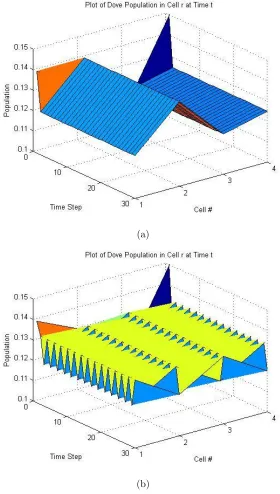
unstable. Consider the example whereα =m= 0.5 and we have a spatial region of

six cells. Sinceα = 0.5, then the equilibirum point is 0,1₂,1₂. With six spatial cells, this translates to each cell having the following population distribution: 0 Hawks, ₁₂1 Doves, and ₁₂1 Retaliators.

If we introduce no diffusion in the system, we get the behavior that we expect

from the equilibirum point: for all timet, in all cellsr, the population distribution is

constant, unchanged from the initial population distribution of 0 Hawks, ₁₂1 Doves, and ₁₂1 Retaliators in each cell. We perturb the initial population distribution by altering only the values of the Doves and Retaliators in each cell. The dynamic using

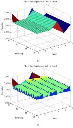
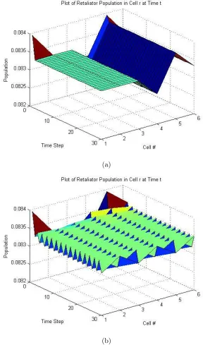
this perturbed initial distribution reaches spatial equilibrium as indicated by Figure

4-1(a) and Figure 4-2(a). In both figures, the Dove and the Retaliator populations

in each cell becomes stable over time.

Without diffusion, the system reaches a stable spatial distribution of the

pop-ulation. Once we introduce diffusion into the system, the system is not able to

reach a spatial equilibirum as shown in Figure 4-1(b) and Figure 4-2(b). Both the

Dove and the Retaliator population in each cell oscillates between 0.0832 and 0.0835

indefinitely. This is an example of spatial instability.

Recall that Turing instability occurs when a temporally stable equilibrium

be-comes spatially unstable. Since (0, α,1−α) has an eigenvalue of 1, it fails the linear

stability test and we cannot be certain that this equilibrium point is linear

tempo-rally stable or not. Hence, we cannot use this as an example of Turing instability

(44)

we are looking for when searching for Turing instability.

4.4

Turing Instability in the Four-Dimensional Case

Consider the following four-dimensional discrete replicator system:

x1(t+ 1) =x1(t)

(A~x)1

~ xT_A_~_x

x2(t+ 1) =x2(t)

(A~x)2

~ xT_A_~_x

x3(t+ 1) =x3(t)

(A~x)3

~ xT_A_~_x

x4(t+ 1) =x4(t)

(A~x)4

~ xT_A_~_x

where(A) is the following fitness matrix

       

0 1 +m 0 1 +m

1−m 1 1 1−m

0 1 1 1 +m

1−m 1 +m 1−m 1−m

       

with 0 < m < 1. This system describes the dynamics of interaction between four

behavior tendencies: Hawks (x1(t)), Doves (x2(t)), Retaliators (x3(t)), and Bullies

(x4(t)).

The equilibirum points of the system and their corresponding eigenvalues are

(45)

(1,0,0,0) Singularity (Division by 0) Numerical results

suggest instability

(0,1,0,0) 0, 1, 1 +m, 1 +m Unstable Equilbirum Point

(0,0,1,0) 0, 0, 1−m, 1 Inconclusive

(0,0,0,1) 0, 1, −_m1−₋m₁ , −_m1−₋m₁ Unstable Equilibrium Point (m,1−m,0) 0, ₁₊1_m, ₁₊1_m, 2₁₊m+1_m Unstable Equilibrium Point (0, α,1−α,0) 0, 1, α(1 +m), 1 +m(2α−1) Unstable Equilbirum Point

0< α <1 if ₁₊1_m < α <1

2m

1+m,0,0,

1−m

1+m

0, 1, 1, 1₁₊−m_m Inconclusive

Since there is no linear temporally-stable equilibrium points in the four-dimensional

(46)

(a)

[image:46.612.153.438.98.595.2]

(b)

(47)

(a)

[image:47.612.153.441.100.589.2]

(b)

(48)

Chapter 5

Using Diffusion to Create Stable

Equilibrium Points

Consider a related problem. Instead of looking for Turing instability, let’s consider

whether it is possible to use diffusion to force a temporally unstable equilibrium

point to become spatially stable. Recall that the Jacobian evaluated at a temporally

unstable equilibrium point has at least one eigenvalue whose magnitude is greater

than 1. Thus, we want to use diffusion to force the magnitude of all eigenvalues to

be less than 1. This is slightly more complex than it seems.

Recall that when we incorporate diffusion into the dynamical system, we

intro-duced spatial cells, each of which could be considered its own dynamical system. We

have to check whether diffusion will turn the eigenvalues of the unstable equilibrium

point in each cell into a stable equilibrium point.

To perform this analysis, we follow a procedure similar to the approach used to

check for the presence of Turing Instability in the three-dimensional case. That is,

(49)

incor-porate diffusion into the matrix (by multiplying the Jacobian with the corresponding

diagonal diffusion matrix), get the corresponding eigenvalues, then see what diffusion

coefficients will force stability.

From the 3-d and the 4-d cases, we will be considering the following equilibrium

points:

(0,1,0) 0, 1 +m, 1 Unstable Equilbirum Point

(0, α,1−α) 0, α(1 +m), 1 Unstable Equilbirum Point

0< α <1 if ₁₊1_m < α <1

(0,1,0,0) 0, 1, 1 +m, 1 +m Unstable Equilbirum Point

(0,0,0,1) 0, 1, −_m1−₋m₁ , −_m1−₋m₁ Unstable Equilibrium Point (m,1−m,0) 0, ₁₊1_m, ₁₊1_m, 2₁₊m+1_m Unstable Equilibrium Point (0, α,1−α,0) 0, 1, α(1 +m), 1 +m(2α−1) Unstable Equilbirum Point

0< α <1 if ₁₊1_m < α <1

For each equilibrium point, we compute (3.2) by mulitplying the Jacobian, J

evalu-ated at that equilibrium point with the appropriate diagonal diffusion matrix. Next,

we compute the eigenvalues of (3.2), which are listed as follows:

Equilibrium Point Eigenvalues

(0,1,0) 0,D1(1 +m), D3

(0, α,1−α) 0, D1α(1 +m), D3α+D2−D2α

(0,1,0,0) 0,D3, D1(1 +m), D4(1 +m)

(0,0,0,1) 0, D2,

−D1(1+m)

m−1 ,

−D3(1+m)

m−1

(m,1−m,0) 0, D3

1+m,

D2m+D1−D1m

1+m ,

D4(2m+1)

1+m

(50)

where Di = 1−4disin2 rπ_k

∈ [−1,1] and di ∈ [0,0.5] for i = 1,· · ·,4. In order

to force an temporally unstable equlibirum point to become spatially stable, the

magnitude of each corresponding eigenvalue must be less than 1.

Consider the case where an equilibrium point has an eigenvalue Di for some

i= 1,· · · ,4. For spatial stability, we want

|Di|<1

to hold for all spatial cells r, 1 ≤ r ≤ k. Note that in the kth _{cell, regardless}

of the di value, Di = 1 since sin2 kπ_k

= 0 It is impossible to force the unstable

equilibrium point in the last (kth_{) cell to become stable. Therefore, it is not possible}

for a temporally-unstable equilbirium point to become spatially stable if they have

Di as an eigenvalue. This allows us to eliminate several cases, leaving only three

equilibrium points to consider.

Consider the point (m,1−m,0,0), which has the D4(2m+1)

1+m eigenvalue. For spatial

stability, we want

D4(2m+1)

1+m

<1

−1< D4(2m+1)

1+m <1 −(1 +m)

1 + 2m < D4 <

(1 +m) 1 + 2m

−(1 +m)

1 + 2m < 1−4d4sin

2 rπ k

< (1 +m)

1 + 2m

−(2 + 3m)

1 + 2m < −4d4sin

2 rπ k

< (−m)

1 + 2m m

4(1 + 2m) < d4sin

2 rπ k

< (2 + 3m)

4(1 + 2m)

Since 0 < m < 1, d4sin2 rπ_k

(51)

hold for the kth _{cell, regardless of the} _d

4 value, since sin2 kπ_k

= 0. Therefore, it is

not possible to force (m,1−m,0,0) to become spatially stable.

Consider the two equilibirum points (0, α,1−α) and (0, α,1−α,0), both of which

have D1α(1 +m) as an eigenvalue. Since we are considering temporally unstable

equilibrium points, α > ₁₊1_m. For spatial stability, we need

|D1α(1 +m)|<1

Since α > ₁₊1_m, let α(1 +m) = x >1. Then we need

|D1x| <1

−1< D1x <1

−1

x < D1 <

1

x

−1

x < 1−4d1sin

2 rπ k

< 1 x

−(1 +x)

x < −4d1sin

2 rπ k

< 1−x x x−1

4x < d1sin

2 rπ k

< 1 +x

4x

Sincex >1,d1sin2 rπ_k

must be positive. However, this inequality will not hold for

the kth _{cell, regardless of the} _d

i value, since sin2 kπ_k

= 0. Hence, it is not possible

to make the equilibirum points (0, α,1−α) and (0, α,1−α,0) spatially stable using

diffusion.

None of the temporally unstable equilibrium points became spatially stable.

Thus, one might conclude that diffusion cannot be used to turn a temporally unstable

equilibrium point a spatially stable equilibrium point.

(52)

in-dicates that we have constant population values for all time t. Thus, it remains to

see whether the spatial distribution of the population across thek cells remains

con-stant (indicating spatial stability) or if populations continue to migrate to different

cells over time, (indicating Turing instability). However, if an equilibrium point is

temporally unstable, then the population values will continue to change over time.

Hence, the spatial distribution of these population values will also change over time,

(53)

Chapter 6

Conclusion

The paper aimed to discuss discrete replicator systems and to explore the parameter

space for instances of Turing instability. We presented the formal definition of the

dis-crete replicator dynamic and introduced a framework story connecting the replicator

dynamic to evolutionary game theory through which we would analyze the system.

The framework story enabled us to replace two parameters from the system with

a dimensionless parameter. We found the equilibrium points for the 2-dimensional,

3-dimensional, and 4-dimensional replicator systems. We introduced diffusion into

a general discrete dynamical system and derived a new Jacobian matrix to aid us

when searching for Turing instability. Finally, we proved that Turing instability was

not possible in the two-dimensional replicator system and showed it was unlikely to

occur in the three-dimensional and the four-dimensional replicator systems. We also

showed that it was not possible to use diffusion for a similar problem: changing a

temporally unstable equilibrium point into a spatially stable equilibrium point.

Based on our work, we conjecture that it will be impossible to use diffusion to

(54)

to cause Turing instability in the replicator system constructed in Chapter 2.

Re-call that when we constructed the fitness matrix, we assumed if a conflict occurs,

the participants have a 50% chance of winning the fight and gaining access to the

resource. It may be possible to achieve Turing instability in a different replicator

system using a fitness matrix where individuals have unequal chances of winning or

losing a conflict.

The possibility of unequal chances of conflict outcomes poses a new area of

re-search. In essence, this means considering different fitness matrices and analyzing

their corresponding equilibrium points. In addition, although we proved that linear

Turing instability was not possible in the two-dimensional, three dimensional, and

four-dimensional cases, we did provide an example of where Turing instability might

occur in the three-dimensional case if we consider equilibrium points with at least one

eigenvalue of magnitude 1. This presents another possible area to explore: looking

beyond linear stability analysis to nonlinear stability analysis in order to find Turing

(55)

Appendix A

Matlab Programs

A.1

Replicator Dynamics

A.1.1

2-dimensional

%Function that performs n steps of the 2d replicator system

%Inputs: parameter m, initial population [x, y], # time steps n

function[pop] = RepEqu2d(m, intpop, n)

%Initalizing the population matrix

pop = zeros(n+1, 2);

pop(1,:) = intpop;

%Constructing the fitness matrix

A = [0 (1+m); (1-m) 1];

a11 = A(1,1); a12 = A(1,2);

(56)

for i=2:n+1

%Constructing the denominator

popvect = [pop(i-1,1); pop(i-1,2)];

denom = popvect’*A*popvect;

%Generating the population vector

x = pop(i-1, 1)*(a11*pop(i-1,1)+a12*pop(i-1,2));

y = pop(i-1, 2)*(a21*pop(i-1,1)+a22*pop(i-1,2));

pop(i,1) = x/denom;

pop(i,2) = y/denom;

total = sum(pop(i,1)+pop(i,2));

pop(i,:) = pop(i,:)/total;

end

%Plotting the populations

figure

plot([0:1:n], pop(:,1), [0:1:n], pop(:,2))

xlabel(’Time’)

ylabel(’Population’)

title(’Population Change over Time’)

legend(’Hawk Population’,’Dove Population’)

axis([0 n 0 1])

(57)

A.1.2

3-dimensional

%Inputs: parameter m, initial population [x, y, z], # time steps n

pop(1,:) = intpop;

A = [0 (1+m) 0; (1-m) 1 1; 0 1 1];

a11 = A(1,1); a12 = A(1,2); a13 = A(1,3);

a21 = A(2,1); a22 = A(2,2); a23 = A(2,3);

a31 = A(3,1); a32 = A(3,2); a33 = A(3,3);

for i=2:n+1

popvect = [pop(i-1,1); pop(i-1,2); pop(i-1,3)];

x = pop(i-1, 1)*(a11*pop(i-1,1)+a12*pop(i-1,2)+a13*pop(i-1,3));

y = pop(i-1, 2)*(a21*pop(i-1,1)+a22*pop(i-1,2)+a23*pop(i-1,3));

z = pop(i-1, 3)*(a31*pop(i-1,1)+a32*pop(i-1,2)+a33*pop(i-1,3));

pop(i,1) = x/denom;

pop(i,2) = y/denom;

(58)

total = sum(pop(i,1)+pop(i,2)+pop(i,3));

end

%Plotting the populations

figure

plot([0:1:n], pop(:,1), [0:1:n], pop(:,2), [0:1:n], pop(:,3))

xlabel(’Time’)

legend(’Hawk Population’,’Dove Population’,’Retaliator Population’)

axis([0 n 0 1])

end

A.1.3

4-dimensional

%Inputs: parameter m, initial population [x, y, z, w], # time steps n

pop(1,:) = intpop;

(59)

0, 1, 1, 1+m; 1-m, 1+m, 1-m, 1-m];

a11 = A(1,1); a12 = A(1,2); a13 = A(1,3); a14 = A(1,4);

a21 = A(2,1); a22 = A(2,2); a23 = A(2,3); a24 = A(2,4);

a31 = A(3,1); a32 = A(3,2); a33 = A(3,3); a34 = A(3,4);

a41 = A(4,1); a42 = A(4,2); a43 = A(4,3); a44 = A(4,4);

for i=2:n+1

popvect = [pop(i-1,1); pop(i-1,2); pop(i-1,3); pop(i-1,4)];

x = pop(i-1, 1)*(a11*pop(i-1,1)+a12*pop(i-1,2)+a13*pop(i-1,3)+...

a14*pop(i-1,4));

y = pop(i-1, 2)*(a21*pop(i-1,1)+a22*pop(i-1,2)+a23*pop(i-1,3)+...

a24*pop(i-1,4));

z = pop(i-1, 3)*(a31*pop(i-1,1)+a32*pop(i-1,2)+a33*pop(i-1,3)+...

a34*pop(i-1,4));

w = pop(i-1, 4)*(a41*pop(i-1,1)+a42*pop(i-1,2)+a43*pop(i-1,3)+...

a44*pop(i-1,4));

pop(i,1) = x/denom;

pop(i,2) = y/denom;

pop(i,3) = z/denom;

pop(i,4) = w/denom;

total = sum(pop(i,1)+pop(i,2)+pop(i,3)+pop(i,4));

(60)

%Plotting the popluations

figure

plot([0:1:n], pop(:,1), ’-’, [0:1:n], pop(:,2), ’:’, ...

[0:1:n], pop(:,3), ’-.’, [0:1:n], pop(:,4), ’--’)

xlabel(’Time’)

legend(’Hawk Population’,’Dove Population’,...

’Retaliator Population’, ’Bully Population’)

axis([0 n 0 1])

end

A.2

Reaction-Diffusion Replicator Dynamics

Note: in the next three programs, the inital population distribution will be entered

as am-by-n matrix where theijth _{entry denotes the initial value for the} _ith_behavior

type in the jth cell, 1≤j ≤n.

A.2.1

2-dimensional

%Function that constructs spatial cells and

%computes population growth for 2d Replicator Dynamics

%Input: parameter m 0<m<1, initial population intpop, number of

(61)

function[x, y] = RepRD2d(A, intpop, n, D)

%Unpacking Diffusion coefficients

Dx = D(1); Dy = D(2);

%Error checking

if size(intpop,1) ~=2

fprintf(’Initial population vector must have only 2 rows.\n’)

return

end

if Dx<0 || Dx>.5 || Dy<0 || Dy>.5

fprintf(’Both diffusion coefficients must be within [0, .5].\n’)

return

end

A = [0 1+m; 1-m 1];

%Gets the number of spatial cells as determined by initial pop vector

r = size(intpop, 2);

%Constructing matrices to store population values

x = zeros(n+1, r); y = zeros(n+1, r);

%Initalizing the 0th row to represent initial distributions

x(1,:) = intpop(1,:); y(1,:) = intpop(2,:);

%Interating through n time steps

for i=2:n+1

%Interating through r spatial cells

(62)

%Dealing with boundary conditions

if j==1

jm1 = r; jp1 = 2;

elseif j==r

jm1 = r-1; jp1 = 1;

else

jm1 = j-1; jp1 = j+1;

end

%Constructing the denominators of r, r-1, and r+1 cells

denom = [x(i-1,j) y(i-1,j)]*A*[x(i-1,j);y(i-1,j)];

denom_m1 = [x(i-1,jm1) y(i-1,jm1)]*A*[x(i-1,jm1);y(i-1,jm1)];

denom_p1 = [x(i-1,jp1) y(i-1,jp1)]*A*[x(i-1,jp1);y(i-1,jp1)];

%Computing the population values

x(i,j) = x(i-1,j)*(A(1,1)*x(i-1,j) + A(1,2)*y(i-1,j));

x(i,j) = x(i,j)/denom;

y(i,j) = y(i-1,j)*(A(2,1)*x(i-1,j) + A(2,2)*y(i-1,j));

y(i,j) = y(i,j)/denom;

%Computing diffusion terms for the x population

if Dx ~= 0

%Computing the r-1 cell population

xm1 = x(i-1,jm1)*(A(1,1)*x(i-1,jm1) + A(1,2)*y(i-1,jm1));

xm1 = xm1/denom_m1;

%Computing the r+1 cell populations

xp1 = x(i-1,jp1)*(A(1,1)*x(i-1,jp1) + A(1,2)*y(i-1,jp1));

xp1 = xp1/denom_p1;

(63)

xdiff = Dx*(xm1 - 2*x(i,j) + xp1);

%Adding Diffusion terms to r cell populations

x(i,j) = x(i,j) + xdiff;

end

%Computing diffusion terms for the y population

if Dy ~= 0

%Computing the r-1 cell population

ym1 = y(i-1,jm1)*(A(2,1)*x(i-1,jm1) + A(2,2)*y(i-1,jm1));

ym1 = ym1/denom_m1;

%Computing the r+1 cell population

yp1 = y(i-1,jp1)*(A(2,1)*x(i-1,jp1) + A(2,2)*y(i-1,jp1));

yp1 = yp1/denom_p1;

%Computing Diffusion terms

ydiff = Dy*(ym1 - 2*y(i,j) + yp1);

%Adding Diffusion terms to r cell populations

y(i,j) = y(i,j) + ydiff;

end

end %End of loop through space

%Rescale the population vector so it adds up to 1

total = sum(x(i,:)) + sum(y(i,:));

x(i,:) = x(i,:)/total;

y(i,:) = y(i,:)/total;

end %End of loop through time

%Generating 3d plots to show population values

(64)

subplot(1, 2, 1)

surf(x([n+1:-1:1],:))

ylabel(’Time Step’)

xlabel(’Cell #’)

zlabel(’Population’)

title(’Plot of Population X in Cell r at Time t’)

subplot(1,2,2)

surf(y([n+1:-1:1],:))

ylabel(’Time Step’)

xlabel(’Cell #’)

zlabel(’Population’)

title(’Plot of Population Y in Cell r at Time t’)

A.2.2

3-dimensional

%Function for constructing spatial cells and

%computing population growth for 3d replicator dynamics

%Input: parameter m, 0<m<1, initial population intpop,

% # time steps n, diffusion coefficient vector [d_1, d_2, d_3]

function[x, y, z] = RepRD3d(m, intpop, n, D)

%Unpacking Diffusion coefficients

Dx = D(1); Dy = D(2); Dz = D(3);

%Error checking

(65)

fprintf(’m must be between 0 and 1 exclusive.\n’)

return

end

if size(intpop,1) ~=3

fprintf(’Initial population vector must have only 3 rows.\n’)

return

end

if Dx<0 || Dx>.5 || Dy<0 || Dy>.5 || Dz<0 || Dz>.5

fprintf(’All diffusion coefficients must be within [0, .5].\n’)

return

end

A = [0 1+m 0; 1-m 1 1; 0 1 1];

%Gets the number of spatial cells determined by initial pop vector

r = size(intpop, 2);

%Constructing matrices to store population values

x

Turing instability in discrete replicator systems

Rochester Institute of Technology

Alex J. Bryce

April 15, 2011

Abstract

Contents

List of Figures

Chapter 1

Chapter 2

Equilibirum Points for the Replicator Dynamic

Replicator Dynamic Examples

Chapter 3

Constructing the Reaction-Diffusion System

Chapter 4

Turing Instability in the Two-Dimensional Case

Turing Instability in the Three-Dimensional

Turing Instability in the Four-Dimensional Case

Chapter 5

Chapter 6

Appendix A

3-dimensional

4-dimensional

Reaction-Diffusion Replicator Dynamics

3-dimensional