City, University of London Institutional Repository
Citation
:
Caudrelier, V. and Doyon, B. (2015). The Quench Map in an Integrable Classical Field Theory: Nonlinear Schrödinger Equation. ..This is the accepted version of the paper.
This version of the publication may differ from the final published
version.
Permanent repository link:
http://openaccess.city.ac.uk/14241/Link to published version
:
Copyright and reuse:
City Research Online aims to make research
outputs of City, University of London available to a wider audience.
Copyright and Moral Rights remain with the author(s) and/or copyright
holders. URLs from City Research Online may be freely distributed and
linked to.
arXiv:1512.08767v1 [math-ph] 29 Dec 2015
The Quench Map in an Integrable Classical Field Theory:
Nonlinear Schr¨
odinger Equation
Vincent Caudrelier
aand Benjamin Doyon
baDepartment of Mathematics, City University London,
Northampton Square, EC1V 0HB London, United Kingdom
bDepartment of Mathematics, King’s College London,
Strand, WC2R 2LS, London, United Kingdom
Abstract
We study the non-equilibrium dynamics obtained by an abrupt change (aquench) in the parameters of an integrable classical field theory, the nonlinear Schr¨odinger equation. We first consider explicit one-soliton examples, which we fully describe by solving the direct part of the inverse scattering problem. We then develop some aspects of the general theory using elements of the inverse scattering method. For this purpose, we introduce thequench mapwhich acts on the space of scattering data and represents the change of parameter with fixed field configuration (initial condition). We describe some of its analytic properties by implementing a higher level version of the inverse scattering method, and we discuss the applications of Darboux-B¨acklund transformations, Gelfand-Levitan-Marchenko equations and the Rosales series solution to a related, dual quench problem. Finally, we comment on the interplay between quantum and classical tools around the theme of quenches and on the usefulness of the quantization of our classical approach to the quantum quench problem.
E-mail: [email protected] or [email protected], [email protected]
1
Introduction
The study of non-equilibrium systems has received a large amount of attention recently, es-pecially in two areas: that of classical stochastic processes and that of quantum many-body problems. Insisting on Hamiltonian, non-stochastic dynamics, a particular protocol of high in-terest, which has the potential for experimental observations, is that of “quenches”: abrupt changes in the parameters of the system. This has been studied intensively within the context of extended quantum systems, and, especially within the framework of integrability, it led to a large body of theoretical results [1]-[35], see also the reviews [36] and [37]. These protocols pose many questions, including the properties of the dynamics following a quench, as well as the thermalization and (especially in integrable systems) generalized thermalization [5, 6, 34, 35] processes describing the large-time steady state.
It is natural to ask similar questions for Hamiltonian dynamics of extendedclassicalsystems: how does a steady (or perhaps simply evolving) solution to a classical field equation (a partial differential equation in space-time) evolve after a parameter of the equation is abruptly modified? In the realm of classical integrable PDEs, of particular interest is the nonlinear Schr¨odinger equation (NLSE). It is a prototype of such integrable PDEs, and hence has a natural pedagogical status to study new ideas. It also appears in the context of nonlinear optics [38] and water wave phenomena (although, arguably, it might be more realistic to be able to control the parameters to create a quench in a nonlinear optics experiment). In this paper, we will concentrate entirely on the NLSE, and the quench will be with respect to the unique parameter of the NLSE.
Of course, contrary to the situation for many-body quantum systems, the numerical sim-ulation of solutions to classical field equations is much easier, and therefore classical quench dynamics are in principle more accessible numerically. In addition, although not posed in this manner, the question of such classical quenches in integrable field theory has been studied for a long time: it is “simply” a special initial value problem. That is, borrowing the terminology from the quantum arena, an initial state is prepared (the initial condition) that might be a special state for a given value of the parameter in the PDE (e.g. a soliton), and is then evolved according to the same PDE but with a different value of that parameter. The long-time be-haviour of the solution of such initial-value problems is one of the key questions, and in the context of integrable PDEs, powerful methods exist that are related to the inverse scattering method [39, 40,41].
It is worth noting that papers [47, 48] are extremely recent and precisely motivated by the question of quenches. Therefore, we would like to argue that the question of quenches in integrable classical theories could serve as a starting point to stimulate (again) studies in the direct part of the inverse scattering method. In addition, we believe that many ideas recently developed in the quantum context have a clear counterpart in the general theory of classical quenches, and that this interplay may be very fruitful. Indeed, it is well-known that integrable systems share the special trait that many techniques and results “survive” quantization exactly: in a nutshell, the inverse scattering method becomes the quantum inverse scattering method.
From the quantum point of view, the fundamental quantities that can be used to understand the quench dynamics are the overlaps between eigenstates in the pre-quench and post-quench bases; in [23] this idea is developed into the quench action formalism. We will show that the classical analog of these overlaps can likewise be subject to a general theory. To achieve this, we propose for this classical analogue the notion ofquench map, that captures the essence of the quench problem in classical integrable theories from the point of view of the inverse scattering method. The map acts on the space of scattering data and represents a change of parameters (thus a change of the scattering transform) with fixed field configuration (i.e.a prescribed initial condition). The quench map is the basic object for describing classical quenches. We study it through three explicit examples and then in more generality by developing a scattering problem that one could interpret as a “higher-level” version of the usual Lax pair approach. This allows us to establish certain analytic properties that the quench map should satisfy.
Finally, we study a “dual quench” protocol, where the field is abruptly changed while the scattering data are fixed. This is related to the quench map by intertwining with the scattering transform, and has an interpretation, by analogy with the quantum case, as the effect of a slow adiabatic change of the parameter of the NLSE (hence is, in a sense, the dual protocol to that of quenches). We provide some observations about the role of the so-called B¨acklund transformations, the Rosales series representation and the Gelfand-Levitan-Marchenko equation in relation to the dual quench. These considerations are perfectly natural from the classical point of view but perhaps less so from the quantum point of view. Nevertheless, we argue that our results may relate to ideas [17] involving the Zamolodchikov-Faddeev algebra.
scattering method: B¨acklund transformations, Gelfand-Levitan-Marchenko equations and the related Rosales expansion. All these have natural quantum counterparts and we comment on the connection between our classical approach and previous studies in the literature on the quantum quench problem. The last Section contains our conclusions and outlook.
2
Lax pair representation and inverse scattering method for the
NLSE
In this Section we recall the basic theory of the NLSE; this serves to introduce our notation. We consider the NLSE for the complex-valued functionq of the two independent variablesx and t, where the strength of the cubic nonlinearity is parametrized asc2:
i∂tq+∂2xq−2c2|q|2q= 0. (2.1)
The case c ∈ R+ is the defocusing case while the case c ∈ iR+ is the focusing case; c = 0 is
simply the noninteracting or free case. The equation appears as the compatibility condition of an overdetermined linear system characterized by the so-called auxiliary problem for Ψ(x, t)∈C2
[40]
(
Ψx= (−ikσ3+W(x, t))Ψ,
Ψt= (−2ik2σ3+P(x, t, k))Ψ,
(2.2)
where the indices indicate partial derivatives, and the 2×2 matrix-valued functionsW(x, t) and P(x, t, k) form the Lax pair [49] and are given by
W(x, t) =c
0 q(x, t)
q∗(x, t) 0
, P(x, t, k) = 2k W −iWxσ3−iW2σ3. (2.3)
In order to discuss the quench problem we introduce the scattering data associated to the auxiliary problem (2.2). The scattering data can be encoded into a matrix-valued function S(k) (the scattering matrix), as a function of a spectral parameter k ∈R, whose extension to
k ∈ C has particular analytic properties. It forms the basis of the inverse scattering method
(ISM) [39, 40, 41]. In particular, the map from a field configuration x 7→ q(x,0) at a given time (here t= 0), to the scattering data k 7→ S(k) – the direct scattering transform – can be seen as a generalization of the Fourier transform that is well adapted to the nonlinear integrable partial differential equations. Indeed, under time evolution, the scattering data evolve in a simple manner. This simple evolution in principle provides the solution to the problem, as the inverse map – the inverse scattering transform – can be obtained by two main techniques, the Gelfand-Levitan-Marchenko equations or the Riemann-Hilbert factorisation problem (see e.g. [50]).
For the NLSE, the details of the scattering transform depend on the class of functions q(x,0) (and more generally q(x, t)) in which we wish to consider the problem. The two classes we consider in this paper correspond to the Schwarz class, and the so-called finite density class [50]. In the former class, the rapidly decreasing case, we impose q as well as all of its higher x-derivatives to vanish as |x| → ∞ faster than any polynomial. In the latter class, we impose instead
lim
x→±∞q(x, t) =ρe
in the sense that q−ρeiθ± is of Schwarz type as x → ±∞. Note that this is compatible with (2.1) providedθ±(t) is linear intand the differenceθ+−θ− is constant. Therefore, in this case,
it is convenient to take θ− = 0 and θ+ = θ a constant in [0,2π), and to consider the gauged
transformed NLSE
i∂tq+∂x2q−2c2(|q|2−ρ2)q= 0, (2.5)
related to the NLSE via q(x, t)7→e−2ic2ρ2tq(x, t). This is incorporated in the auxiliary problem by simply changing P to P +ic2ρ2σ3 while keeping everything else unchanged. In particular,
this does not affect the form of thex-part of the auxiliary problem, which is the important part for computing the scattering data from a given initial condition. The special caseρ = 0 of the finite density class recovers the Schwarz class.
The scattering data is then computed by considering two Jost solutions Ψ±of the x-part of
the auxiliary problem at fixed time with appropriate asymptotics asx→ ±∞. Let us denote
W±:= lim
x→±∞W(x,0), (2.6)
and
E±(x, k) :=P±e−iΛ±(k)x (2.7)
the solution of
Ex+ (ikσ3−W±)E= 0, E(0, k) = 1I2, (2.8)
where we have assumed thatikσ3−W±is diagonalizable toiΛ±(k) via the matrixP± and where
1I2 is the unit 2×2 matrix. Then, the Jost solutions Ψ±= Ψ±(x, k) are defined as the unique
solutions to
Ψx+ikσ3Ψ =W(x,0)Ψ (2.9)
satisfying the asymptotic conditions
lim
x→±∞E −1
± (x, k)Ψ±(x, k) = 1I2. (2.10)
The scattering matrix S(k) is then the matrix connecting the two Jost solutions according to
Ψ+(x, k) = Ψ−(x, k)S(k). (2.11)
In practice, we can compute it as follows
S(k) = lim
x→−∞E −1
− (x, k)Ψ+(x, k). (2.12)
The spectral parameter takes values in k ∈ Rρ, where Rρ is R in the rapidly decreasing case,
and isRminus a fixed interval depending on ρin the finite density case [50]. The task is further
simplified by noting that there is a symmetry of the auxiliary problem that follows from the property
W∗ =σ W σ , (2.13)
where
σ =
0 c /|c|
c∗/|c| 0
. (2.14)
This implies the following form for S(k):
S(k) =
a∗(k) b(k)
c∗
c b∗(k) a(k)
Combined with the fact that S(k) has unit determinant, this involution property has a more transparent form in the focusing case,
S†(k) =S−1(k) (k∈Rρ), (2.16)
showing thatS(k) is in the groupSU(2) for each k∈Rρ. The details of the involution on the
spectral parameter k depend on the class we are working in and will be clear in the examples below. Further details can be found in [50]. The main observation for our purposes is that it is enough to compute aand bin order to completely characterize the direct scattering transform. Finally, the scattering dataS(k) evolves in a simple manner under the time evolution determined by the NLSE (2.1) (or (2.5) in the finite-density case):
S(k;t) =e2ik2tσ3S(k)e−2ik2tσ3. (2.17)
3
General ideas and the quench map
Following the usual implementation of a quench, one first assumes that the field configuration q(x, t) is a stationary, or in some way natural, solution to the NLSE, with parameter c, for all times t < 0. In quantum problems, one often takes the ground state of a given many-body Hamiltonian; in the present case, one may instead assume the presence of one or a finite number of solitons, or a stationary extrapolating solution in the finite-density case (the zero-field solution q= 0, in the Schwartz case, would give a trivial quench). Then, an abrupt change c7→c′ of the parameter is performed. This is implemented by considering q(x,0) as the initial condition for a new time evolution, corresponding to the NLSE with this modified parameter. The solution q(x, t) for all t > 0 is determined by solving the NLSE with parameter c′, from the initial conditionq(x,0) (which, we emphasize, was assumed to be a natural solution to the NLSE with parameterc).
Since the time evolution (2.17) is simple in the space of the scattering data, it is convenient to recast the quench problem to that space. Denote by
Fc :{x7→q(x)} → {k7→S(k)} (3.1)
the direct scattering map with parameter c, from field configurations to scattering data, as defined by (2.12). Since q(x, t), t < 0 is a natural solution to the NLSE with coupling c, the scattering dataS(k) =S(k, c) :=Fc[q(·,0)](k) is assumed to be known and simple, and the time
evolution ofS(k, c) fort <0 is given by (2.17). The time evolution ofS(k, c) fort >0 is however not simple, as it is performed by using the NLSE with parameter c′ 6=c. In order to solve the
quench problem in the space of scattering data, we need to obtain S(k, c′) := F
c′[q(·,0)](k). OnceS(k, c′) is evaluated, the quench problem is in principle solved, as the evolution of the new
scattering data for t > 0 is again given by (2.17). The inverse scattering method, which gives the inverse transform Fc−1′ , then allows one to recover q(x, t) for t >0.
Let us introduce the quench mapas the bijective map1
Qc′,c=Fc′◦ Fc−1 (3.2)
1Bijectivity of F
on the space of scattering data. The full time evolution in this space is then
S(k;t) =
(
e2ik2tσ
3S(k)e−2ik2tσ3 t <0
e2ik2tσ3Q
c′,c[S](k)e−2ik
2tσ
3 t >0 (3.3)
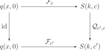
where S(k) = S(k, c). The quench problem at the time t= 0 can be visualised as the commu-tative diagram in Figure 1. Hence, the knowledge of the quench map is in principle enough to
q(x,0) Fc ✲S(k, c)
q(x,0) id
❄
Fc′
✲ S(k, c′)
Qc′,c
[image:8.595.213.383.220.303.2]❄
Figure 1: The quench problem in scattering data space.
solve the quench problem. In Section 5, we explore the relation between the quench map and the inverse scattering method, and show that it leads to a sort of higer-level auxiliary problem
that captures some of the properties of the quench mapQc′,c.
In the quantum quench problem, the important objects are the overlaps between the eigen-states of the initial and final Hamiltonians. It is natural to interpret the quench mapQc′,cas the classical analogue of such overlaps. Indeed, the field q(x) is interpreted as the quantum state, and the scattering dataS(k, c) (S(k, c′)) as the coefficients of the state in the basis of eigenstates
of the initial (final) Hamiltonian. The overlaps between the eigenstates of the initial and final Hamiltonians allow one to go from one basis to the other, and thus their classical analogue is the quench map.
Remark 3.1 The quench map has obvious group properties
Qc,c= id , Qc′′,c′◦ Qc′,c=Qc′′,c , Q−1
c′,c=Qc,c′. (3.4)
For any given c0, we may define Qc :=Qc,c0 and we have Qc′,c=Qc′ ◦ Q
−1
c . In the case of the
NLSE, we may always rescale the field q → p|c|q when c6= 0, so that we can always consider the quench problem with |c0|= 1: the normalized quench problem.
From the point of view of the inverse scattering method, it is important to realise that the quench problem is completely solved if we can implement explicitely thedirect part of the inverse scattering method, that is, if we can compute the scattering dataS(k, c) for fixed but arbitrary c, given an initial condition q(x,0). Indeed, this amounts to finding Fc for all values of c and
then the map Qc for the normalized quench problem is obtained from
Qc =Fc◦ Fc−10 . (3.5)
To our knowledge, the following references exhaust all such studies in the case of NLSE. The first occurence is [44] and, independently it seems [45], for the focusing case with vanishing boundary conditions and for a choice of initial data corresponding to a one-soliton solution. Recently, other forms of the initial data were considered in [46] also in the focusing case with vanishing boundary conditions. Much more recently, the same question was solved in [47] in the defocusing, finite density case and for a choice of initial data corresponding to a soliton solution. While finalizing this paper, we discovered [48] that tackles the quench problem for a variety of integrable classical field theories, but restricted to very specific initial conditions. In the following Section, we reproduce the original approach of [44,45] to obtain Fc and adapt it
to obtain the results presented in [47] (now also available in the very recent preprint [48]). We also give a new example corresponding to the focusing case at finite density. All three cases cases share common mathematical features but their physical relevance is quite different.
4
Calculations of the quenched scattering data in the NLSE
In this Section we set out to compute the scattering data S(k, c) explicitely as in (2.12) in three different situations: rapidly decreasing focusing NLSE, finite density focusing and defocusing NLSE. In each case the initial condition is chosen to be precisely of soliton type for the normalized value of the paramter (c0 = i or c0 = 1). This gives us the value of the quench map at three
specific points in the scattering data space.
4.1 Rapidly decreasing case
Let us compute the scattering data explicitly starting from the initial data
q(x,0) =A e
i(V x+φ0)
cosh (A(x−x0))
, (4.1)
which corresponds to a one-soliton solution of the focusing NLSE (c0 = i) with amplitude A,
velocity V and some arbitrary phase and position shifts φ0 and x0. The latter can be set to
zero without loss of generality. The case V = 0 was considered in [45] and restricted there to the focusing case c∈iR. Here, we make no such restrictions since it turns out that the results
hold in general. For this case, we haveW±= 0 and hence
λ±(k) =kσ3 , P±= 1I2 (4.2)
so that (2.12) yields
b(k, c) a(k, c)
= lim
x→−∞
φ+12(x, k) φ+22(x, k)
, (4.3)
whereφ+(x, k) =e−ikxσ3Ψ+(x, k). Let us setz(x) = 12(1−tanhAx) and
F(z) =φ+22(x, k). (4.4)
This yields,
φ+12(x, k) = e
2ikx
cq∗(x,0)
dz dxF
′
Inserting in ∂xφ+12(x, k) = cq(x,0)e2ikxφ+22(x, k), we get, after some algebra involving standard
hyperbolic identities
z(1−z)F′′(z) +
1 2 − i A
k+V
2
−z
F′(z)−c2F(z) = 0. (4.6)
Therefore, one finds thatF is the solution of the hypergeometric differential equation
z(1−z)F′′(z) + [γ−(α+β+ 1)z]F′(z)−αβF(z) = 0. (4.7)
withβ =−α, α2 =−c2,γ = 12 −Ai k+V2 . The change α→ −α has no effect so we can set
α=ic. The boundary conditions coming from
lim
x→∞φ +
22(x, k) = 1 , xlim→∞φ+12(x, k) = 0, (4.8)
read
F(0) = 1 , lim
z→0z
1
2−
i A(k+
V
2)F
′
(z) = 0. (4.9)
Therefore, we find
F(z) =2F1
ic,−ic,1
2−
i A
k+V
2
;z
. (4.10)
Taking the limit of the functions in (4.4)-(4.5) as x→ −∞,i.e.z→1, we obtain after simplifi-cation,
a(k, c) = Γ
1 2 −
i A k+
V
2 2
Γ 12 −ic−Ai k+V2Γ 12 +ic−Ai k+V2, (4.11)
b(k, c) = −sin(iπc)
ic
1
coshπA k+V2, (4.12)
where Γ is the Gamma function. When c = i, we consistently recover the scattering data corresponding to the one-soliton solution of NLSE, that is
b(k, i) = 0 , a(k, i) = k−k1
k−k∗ 1
, k1 =−
V
2 +
iA
2 . (4.13)
Therefore, we get the value of the quench mapQc,i =Qc at the “point” (a(k), b(k)) =
k−k1
k−k∗
1,0
,
Qc
k−k1
k−k∗ 1
,0
= (a(k, c), b(k, c))
= Γ 1−
i
A(k−k1)
2
Γ 1−ic−Ai (k−k1)Γ 1 +ic−Ai (k−k1)
,sin(iπc) ic
i sinhπ
A(k−k1)
!
. (4.14)
Thanks to these explicit expressions, we can investigate in detail the effect of a quench. As noted above, although historically [45] only considered the focusing case, c∈iRhere, it is clear
Focusing to focusing quench In this case, c ∈iR and we set c = iν, ν >0. The system
is quenched for ν 6= 1. Of all these values, we see that the case where ν = n ∈ N is special:
b(k, in) = 0 meaning that q(x, t) is reflectionless i.e. of solitonic type. The corresponding form of a(k, in) is
a(k, in) =
n
Y
j=1
k−kj
k−k∗
j
, kj =−
V
2 +
(2j−1)iA
2 . (4.15)
Note that only the amplitudes change while the velocity remains the same for each zero of
a(k, in): the corresponding solution is a bound state of n solitons moving together with the
same velocity and with a hierarchy of equally spaced amplitudes, separated by A. In general, for non integral values of ν, the zeros of a(k, iν) are located at those values of k = kR+ikI,
kI >0 such that the argument of one the Gamma functions in the denominator is a negative
integer −n,n= 0,1,2, . . .. This yields, remembering thatkI >0, only the following possibility
(
kR=−V2 ,
kI =−A(n+12 −ν).
(4.16)
So if 0 < ν < 1, we see that a(k, iν) has no zero in the upper-half plane. This means that the initial soliton desintegrates into a purely radiative solution controlled by the continuous scattering data ρ(k, c) = ab((k,ck,c)),k∈R. This is reminiscent of the well-known fact that there is
a threshold for the value of the coupling in order to get a soliton in the focusing case. If the quench is to a value of c such that N < ν < N+ 1 for some N ≥1, then a(k, iν) has N zeros forn= 0, . . . , N −1, all having the same real part. The corresponding solution consists of the abovementioned bound state of solitons together with an additional radiative part that decays at large times.
Focusing to defocusing quench In this case, we assume thatc > 0. Performing the same analysis to find the possible zeros of a(k, c) in the upper half-plane, we find no solutions. This is consistent with the known fact that the rapidly decreasing defocusing case does not support discrete eigenvalues leading to solitons. We also see that b(k, c) is never zero in that case. So, we find that a quench to a positive value of the coupling destroys the initial soliton and leaves only a purely radiative solution controlled by ρ(k, c) = ba((k,ck,c)), k∈R. We note that there is an
interesting expression of the solution in that case, which is a special case of the perturbative expansion discovered by Rosales in [51]. It can also be derived using the Neumann series solution to the Gelfand-Levitan-Marchenko equations for the reconstruction ofq(x, t) from the scattering data. This is the object of Section 6.2.
Focusing to free quench It is interesting to study the special limit when the coupling goes to zeroi.e.the limiting case of the free Schr¨odinger equation. Solitons do not exist in this regime since they are purely nonlinear objects. Moreover, the inverse scattering method is known to boil down to the usual Fourier transform in this case. So we expect a(k,0) to be simply 1 and b(k,0) to be essentially the Fourier transform of q(x,0). In this limit, it is readily checked that a(k,0) = 1 and
b(k,0) =− π
coshAπ k+V2. (4.17)
definition of the scattering matrix fromφ+ asx→ ∞. Explicitly, we can keep track of the small c limit by writing
Ψ+(x, k) =e−ikxσ3(1I
2+cK(x, k) +O(c2)), (4.18)
and inserting in (2.2). Keeping the first order inc, we get
Kx(x, k) =
0 e2ikxq(x,0)
e−2ikxq∗(x,0) 0
. (4.19)
This yields, using the normalization of Ψ+ asx→ ∞,
K(x, k) =
0 −Rx∞e2ikξq(ξ,0)dξ
−Rx∞e−2ikξq∗(ξ,0)dξ 0
. (4.20)
The entry (12) in this matrix coincides with b(k,0) as x → −∞ according to the definition of S(k, c) and is indeed seen to be exactly the Fourier transform of the initial data (up to the minor modifications already mentioned).
4.2 Finite density case with repulsive nonlinearity
In this case, given the asymptotic behaviour (2.4), we see that
W−=c
0 ρ
ρ 0
, W+=ei θ
2σ3W
−e−i θ
2σ3. (4.21)
As a consequence,
Λ+(k) = Λ−(k) =µ(k)σ3, (4.22)
whereµ satisfies
µ2 =k2−c2ρ2, (4.23)
and
P−=e−i θ
2σ3P+ =
1 i(µcρ−k)
−i(µcρ−k) 1
!
(4.24)
Let us discuss the quench problem using as initial data the following one-soliton solution of (2.5) withc= 1 [50]
qF D(x, t) =ρ
1 +eiθeν(x−vt)
1 +eν(x−vt) , (4.25)
withρ >0 and,
v=−2cρcosθ
2 , ν = 2cρsin θ
2. (4.26)
taken at t= 0. Hence, the initial data read
q(x,0) =ρ1 +e
iθeνx
1 +eνx , ν >0. (4.27)
we present this case too with our notations. Since we work with Ψ+, it is convenient to change to the basis where W+ is diagonal, so we set
Φ+(x, k) =P−1e−iθ2σ3Ψ+(x, k). (4.28)
The auxiliary problem can again be mapped to the hypergeometric differential equation by using
w(x) = 1
2(1−tanh νx
2 ), (4.29)
and
ϕ(w) =
Φ+12(x, k) Φ+22(x, k)
≡
ϕ1(w)
ϕ2(w)
. (4.30)
Noting that
q(x,0) =ρ(w+eiθ(1−w)) , dw
dx =−νw(1−w), (4.31)
we obtain dϕ dw = iµ ν 1 wσ3+
1
1−wQ(θ)
−1σ 3Q(θ)
ϕ , (4.32)
where
Q(θ) =
β∗ −α
−α β
, α= cρ
µ sin θ
2 , β = cos
θ 2 +i
k µsin
θ
2. (4.33)
Setting
ϕ(w) =
M1(w)
M2(w)
1−w w
iµν
, (4.34)
we obtain after some algebra, and using the relationββ∗−α2 = 1,
w(1−w)d
2M 2
dw2 −
w+ 2iµ
ν
dM2
dw +c
2M
2= 0. (4.35)
From our normalisation,M2(0) = 1 and we get
M2(w) =2F1
c,−c,−2iµ
ν ;w
, (4.36)
which in turn yields,
M1(w) =
α β∗
2F1
c,−c,−2iµ
ν ;w
−(1−w)2F1
1 +c,1−c,1−2iµ
ν ;w
(4.37)
Therefore, the coefficients a(k, c),b(k, c) are found as
b(k, c) a(k, c) = lim w→1 1−w w 2iµ ν (β∗M
1(w)−αM2(w))
βM2(w)−αM1(w)
!
, (4.38)
and read, after simplification,
a(k, c) = −(
2iµ ν −c)(
2iµ ν +c)
β∗2iµ
ν
2 Γ
2(1−2iµ ν )
Γ(1−2iµν −c)Γ(1−2νiµ+c), (4.39)
b(k, c) = sinπc
πc
sinh2πµν
2πµ ν
!−1
. (4.40)
Defocusing to defocusing quench In this context, integer values ofcproduce reflectionless solutionsb(k, n) = 0. The corresponding coefficienta(k, n) becomes
a(k, n) = 1
β∗
n
Y
m=1
2µ−imν
2µ+i(m−1)ν , (4.41)
showing the location of the zeros (in µ). They correspond to discrete values of k in the gap [−c2ρ2, c2ρ2]. For noninteger values of c, the quench solution combines the previous special multisoliton with a radiative background decaying at large times. More details can be found in [48].
Defocusing to focusing quench If c= iγ,γ > 0, we immediately see that b(k, c) is never zero so that the original reflectionless soliton desintegrates into a radiative solution. This is consistent with the fact thata(k, c) cannot have zeros in that case.
4.3 Finite density case with attractive nonlinearity
For our final example, we present a quench in a novel situation: the finite density case with
attractive nonlinearity, corresponding to the case c0 =i. In [52], the inverse scattering method
and solitons solutions for this case have been studied in detail and a good review of previous results is given. We use the following one-soliton initial profile corresponding to the solution rederived by the authors of [52] as a particular case of their general multisoliton formula. Setting t= 0 as well as ξ=φ= 0 in eq (4.1) of [52], we consider
q(x,0) = cosh(Ax+B)−iA
cosh(Ax+B) , (4.42)
where
A=Z−1/Z , tanhB = C
2−4Z2A2
C2+ 4Z2A2, C =Z+ 1/Z , Z >1. (4.43)
This initial profile corresponds to a stationary soliton on a nonzero constant background (the density ρ = 1 here) and is controlled by one parameter Z > 1. Note that we can always set B = 0 by using a translation inx. Therefore, we consider the initial profile
q(x,0) = 1− iA
coshAx. (4.44)
We follow the same steps as in Section 4.2. We have
W−=W+=c
0 1 1 0
≡c σ , (4.45)
and then,
Λ+(k) = Λ−(k) =µ(k)σ3, (4.46)
whereµ satisfies
µ2 =k2−c2. (4.47)
For convenience, let us writec=ig (so the unquenched situation corresponds to g= 1) and
We have
P−=P+=
1 µ−gk
−µ−gk 1
!
≡P . (4.49)
As before, let us work with the solution Ψ+ of (2.9)-(2.10) and set
Φ+(x, k) =P−1Ψ+(x, k). (4.50)
After some algebra, we find that Φ+ is the solution of
Φx+iµ(k)σ3Φ =gQΦ (4.51)
normalized to lim
x→∞e
iµ(k)xσ3Φ+(x, k) = 1I, where
Q(x) = A
coshAx
0 1
−1 0
(4.52)
This is very similar to the rapidly decreasing case with µ(k) playing the role of k. Thus, the effect of the finite density is encapsulated in a redefinition of the spectral parameterk→µ(k). We simply writeµ in the following. Setting
φ(x, µ) =eiµxσ3Φ+, (4.53)
recall that we want to compute
b(µ, c) a(µ, c)
= lim
x→−∞
φ12(x, µ)
φ22(x, µ)
. (4.54)
From here on, the calculations are similar to the rapidly decreasing case. We set
z(x) = 1
2(1−tanhAx), F(z) =φ22(x, µ). (4.55)
One then finds that F satisfies the hypergeometric differential equation
z(1−z)F′′+
1
2 −i µ
A −z
F′+g2F = 0, (4.56)
with lim
z→0F(z) = 1. The second boundary condition comes from the condition onφ12asx→ ∞
and reads
lim
z→0z
1
2−
iµ A F
′
(z) = 0. (4.57)
Thus,
F(z) =2F1
g,−g,1
2 −
iµ A;z
, (4.58)
and, after simplification (recall c=ig here),
a(µ, c) =
Γ12 −iµA2
Γ12 −g−iµAΓ12 +g− iµA
, (4.59)
b(µ, c) = −sin(πg)
g
1
where Γ is the Gamma function. Wheng= 1, we find the scattering data corresponding to the initial one-soliton solution of the finite density, focusing NLSE equation
b(µ, i) = 0 , a(µ, i) = µ−µ1
µ−µ∗ 1
, µ1 =
iA
2 . (4.61)
Therefore, the quench map Qc,i =Qc reads in this case
(µ−µ1
µ−µ∗
1 ,
0 7→
Γ(1−i
A(µ−µ1))
2
Γ(1−g−Ai(µ−µ1))Γ(1+g−Ai(µ−µ1)),
sin(πg)
g
i
sinhπ A(µ−µ1)
(4.62)
It looks deceptively identical to the rapidly decreasing case but one has to remember that µis a nontrivial function of the original spectral parameter k. The subtleties of the finite density case are contained in the more complicated analytical properties of the scattering data. That being said, the structural form of the scattering coefficients allows one to analyse the focusing to focusing, or focusing to defocusing quench along the same lines as the previous two examples, with the same qualitative conclusions.
4.4 Remarks on the examples
These three examples show striking similarities in the tools employed. In particular, the mapping of the problem to the hypergeometric differential equation is a common feature. One might argue that this is because we have picked a particular soliton solution as initial condition in each scenario. However, the close relationship between soliton theory and connection problems for special functions is well-known. The importance of special functions in the algebro-geometric approach to the inverse scattering method [53,54,55,56] is also well-known and gives hope that one could develop a more systematic theory for the direct part of the inverse scattering method, with applications to a wider class of quench problems.
In the following Section, we leave the arena of specific examples and consider the general problem of characterising the quench map via its spectral analysis.
5
The quench map from the ISM: a general approach
In this Section, we address the question of finding general analytic properties of the quench map by using the full power of the inverse scattering method. For simplicity, we consider only the rapidly decreasing focusing case. Recall that we haveW(x, t)→0 as |x| → ∞. It is convenient to perform a gauge transformation Φ :=eikσ3xΨ. The transformed matrix potential is then
U(x) :=eikσ3xW(x,0)e−ikσ3x =c
0 e2ikxq(x,0)
−e−2ikxq∗(x,0) 0
, (5.1)
where for lightness of notation we keep thekdependence implicit. Note that, forkreal,U†(x) =
−U(x) and Tr(U(x)) = 0; that is,iU is in the fundamental representation of the su(2) algebra. The fundamental solutions Φ± = Φ±(x) to
areSU(2) matrices forkreal. Using the convention of ordering the integrals from right (bottom limit) to left (top limit), the solutions can be written as path-ordered integrals:
Φ−(x) =Pexp Z x
−∞
dy U(y), Φ+(x) =Pexp Z x
∞
dy U(y). (5.3)
The scattering matrix S=S(k) introduced in (2.12) can be written as
S= Φ†−(x)Φ+(x) =Pexp Z −∞
∞
dy U(y) (5.4)
(for any x). We remark that by standard arguments (which we recall below), one may show that the fundamental solutions Φ±, as functions ofk, have the following analytic properties:
(Φ−)11 (Φ+)12
(Φ−)21 (Φ+)22
is analytic for Im(k)>0,
(Φ+)11 (Φ−)12
(Φ+)21 (Φ−)22
is analytic for Im(k)<0
(5.5) for any x∈R.
From the discussion in Section3, the mapFc representing the direct problem with coupling
c, which maps from the space of initial conditionsq(x) to the space of scattering dataS(k), is
Fc :q7→S =Pexp
Z −∞
∞
dy U(y). (5.6)
We are interested in the quench mapQc′,c=Fc′◦ Fc−1. We recall that this acts on the space of scattering data and represents the change of scattering data associated to a change of coupling parameterc7→c′, keeping fixed the initial condition.
Recall the notation from (2.15), with in particulara=S22. We assume thata(k) may only
have finite-order zeroes in the upper half k-plane2. We will show the following:
Proposition 5.1 There exist smooth matrix functions Θǫ(x), ǫ∈ {±}, that also depend on k,
in the fundamental representation of the SU(2) group for x, k∈R, such that
Qc′,c:S 7→S′ = Θ†
−(x)SΘ+(x), (5.7)
where the right-hand side is independent of x∈R. The following analytic properties hold in the
k-plane:
M(x) := 1 a
(S†Θ
−)11 e−2ikx(Θ+)12
e2ikx(Θ−)21 (SΘ+)22
is analytic in k for Im(k)>0 (5.8)
except possibly for isolated singularities at the zeroes of a. The following asymptotic conditions in k and in x hold:
lim
k→i∞M(x) =1I2, xlim→∞Θ+(x) = limx→−∞Θ−(x) =1I2, x→−∞lim SΘ+(x) = limx→∞Θ †
−(x)S. (5.9)
2
Finally, let m(x) be a column vector of M(x), and letk=k0 be a zero ofa(k) in the upper half
k-plane of order j≥1. If we assume that m(x) has a finite-order pole at k=k0 of order ℓ≥0
(or no pole, ℓ= 0), then there exists b0 ∈C such thatm(x) has the form
m(x)∝(k−k0)−ℓ 1 +O(k−k0)
−b0
1
+O(k−k0)j−ℓ 1
b∗ 0
. (5.10)
If the coefficient b(k) in (2.15) can be extended analytically to k0, then b0=b(k0).
With an explicit parametrization
Θ±=
u∗ ± v±
−v∗ ± u±
, |u±|2+|v±|2 = 1, (5.11)
the analyticity conditions (5.8) and the asymptotic conditions in ktranslate into the statement that
u∗−(x) + b av
∗
−(x), e2ikx
1 av
∗
−(x), e−2ikx
1
av+(x), u+(x)− b∗
av+(x) (5.12)
are analytic for Im(k) > 0 except for possible isolated singularities at the zeroes of a(k), and tend to 1, 0, 0 and 1 respectively as k→i∞.
Let us fix x = 0. The above proposition can then be stated as follows: there exists four functions f, g, h and j of the variable k, analytic in the upper half plane except for possible isolated singularities at the zeroes of a, whose limits as k→ i∞ are 1, 0, 0 and 1 respectively, and with the properties that
f f∗+gg∗−gf∗b−f g∗b∗ = 1, hh∗+jj∗+jh∗b+hj∗b∗ = 1, (5.13) and that the possible singularities of the column vectors (f, h)T and (g, j)T, at the zeroes k0 of
a, are described as in (5.10), such that the scattering data after the quench are given by
a′ = (f j−gh)a, b′ =jf∗b+hg∗b∗−jg∗−hf∗. (5.14)
Sketch of the proof. We are looking for an expression forS′=Q
c′,c(S). We will use the notation δc=c′−c. Consider the solutions Θ
ǫ(x), for ǫ∈ {±}, to the scattering equations
∂xΘǫ(x) =
δc
c Uǫ(x)Θǫ(x) (5.15)
with potential
Uǫ(x) = Φ†ǫ(x)U(x)Φǫ(x), (5.16)
normalized as Θǫ(x →ǫ∞) = 1I2. Here and below, except when explicitly displayed or stated,
U(x) and Φǫ(x) are evaluated atc.
Note that U(x, c′) = (c′/c)U(x, c). Using this simple relation along with (5.2) and the uniqueness of the initial value problems, we deduce that
Θ−(x) = Φ†−(x, c)Φ−(x, c′), Θ+(x) = Φ†+(x, c)Φ+(x, c′). (5.17)
Then, from (5.4) we remark that
Setting Θǫ= Θǫ(x) for anyx∈R, we have (5.7). We now use the scattering problems (5.15) in
order to deduce the analytic properties (5.8) of Θǫ as functions ofk.
Recall that one can solve recursively the scattering equation (5.2), with appropriate asymp-totic conditions, by re-writing them in integral form,
Φǫ(x) = 1I2+ Z x
ǫ∞
dy U(y)Φǫ(y). (5.19)
Let us make the transformation:
Φǫ(x) =eikσ3xΦ˜ǫ(x)e−ikσ3x (5.20)
so that
˜
Φǫ(x) = 1I2+ Z x
ǫ∞
dy eikσ3(y−x)W(y) ˜Φ
ǫ(y)e−ikσ3(y−x). (5.21)
Let us define the column vectors fǫη, for η = ±, by ˜Φǫ = (fǫ+,fǫ−). Applying, to the right of
(5.21), the projectors Pη onto the eigenvectors vη of σ3 with eigenvalues η, we conclude that fǫη(x) =vη+
Z x ǫ∞
dy eik(σ3−η)(y−x)W(y)f
ǫη(y). (5.22)
By standard arguments, recursively solving this integral equation, one deduces the following:
fǫ,−ǫ(x) are analytic ink for Im(k)>0, and tend to v−ǫ ask→+i∞; and fǫǫ(x) are analytic in
kfor Im(k)<0, and tend to vǫ ask→ −i∞; these statements being valid uniformly for x∈R.
This in particular implies (5.5). We remark that, from the representationa= det(f−+,f+−) [50],
one finds that ais analytic in the upper halfk-plane and limk→i∞a(k) = 1.
Similarly, let us re-write equation (5.15), with appropriate asymptotic conditions, as integral equations,
Θǫ(x) = 1I2+
δc c
Z x ǫ∞
dy Uǫ(y)Θǫ(y). (5.23)
Let us introduce the column vectors fǫη by Φǫ = (fǫ+, fǫ−), and recall that S =
a∗ b
−b∗ a
(using (2.15) and c∈iR+), with|a|2+|b|2 = 1. Let us further define
Φ>= (f−+, f+−), Φ<= (f++, f−−), U>= Φ†<UΦ>, U<= Φ†>UΦ<. (5.24)
The relation (5.4) impliesf++=a∗f−+−b∗f−− and f+−=bf−++af−−, and thus we have
Φ+=
1 aΦ>
1 0
−b∗ a
= 1
a∗ Φ<
a∗ b
0 1
, Φ−=
1 aΦ>
a −b
0 1
= 1
a∗Φ<
1 0
b∗ a∗
. (5.25)
From this we remark that
U+ =
1 aJ
−1
+ U>J+=
1 a∗J
†
+U<J+† −1, U−=
1 aJ
−1
− U>J−=
1 a∗J
†
−U<J−† −1 (5.26)
where
J+=
1 0
−b∗ a
=P++P−S, J−=
a −b
0 1
=P−+P+S†. (5.27)
We now define
Applying these similarity transformations to the equation (5.23), we obtain
Θǫκ(x) = 1I2+ δc
c 1 aκ
Z x ǫ∞
dy Uκ(y)Θǫκ(y) (5.29)
whereǫ∈ {±}andκ∈ {>, <}and wherea>=aanda<=a∗.
Let us make the transformation Θǫκ(x) =eikσ3xΘ˜ǫκ(x)e−ikσ3xand Φκ(x) =eikσ3xΦ˜κ(x)e−ikσ3x.
We then obtain
˜
Θǫκ(x) = 1I2+ 1
aκ
Z x ǫ∞
dyδc
c e
ikσ3(y−x)Φ˜†
−κ(y)W(y) ˜Φκ(y) ˜Θǫκ(y)e−ikσ3(y−x) (5.30)
(where here −κ is < (>) ifκ is >(<)). We remark that ˜Φ>(x) = (f−+(x),f+−(x)) is analytic
inkfor Im(k)>0 and tend to 1I2 ask→i∞, and that ˜Φ<(x) = (f++(x),f−−(x)) is analytic in
k for Im(k)< 0 and tend to 1I2 as k→ −i∞ (both uniformly in x). Therefore, by recursively
solving the integral equation and using the fact that a(k) tends to 1 as k → i∞, we conclude that: ˜Θ+>(x)P− and ˜Θ−>(x)P+ are both analytic in k for Im(k) > 0, except possibly at the
positions of the zeroes ofa=a(k) in the upper-half plane, and tend toP− andP+, respectively,
as k → i∞; and that ˜Θ+<(x)P+ and ˜Θ−<(x)P− are both analytic in k for Im(k) <0, except
possibly at the positions of the zeroes ofa∗=a∗(k) in the lower-half plane, and tend toP + and P−, respectively, ask→ −i∞. Clearly, the same analyticity properties hold for
M>(x) :=
X
ǫ
˜
Θǫ>(x)P−ǫ and M<(x) :=
X
ǫ
˜
Θǫ<(x)Pǫ, (5.31)
respectively, with the same asymptotic behaviours as k→ ±i∞. Using the relations
J+−1 = 1
a(P−+S
†P
+), J−−1=
1
a(P++SP−) (5.32)
along with (5.27) one obtain the explicit forms
M>=
1 a
(S†Θ
−)11 e−2ikx(Θ+)12
e2ikx(Θ
−)21 (SΘ+)22
M<=
1 a∗
(SΘ+)11 e−2ikx(Θ−)12
e2ikx(Θ
+)21 (S†Θ−)22
. (5.33)
With the parametrization (5.11), one finds that
M<=σ2M>∗σ2. (5.34)
Therefore, the analyticity and asymptotic conditions on M> and M< are equivalent, and it is
sufficient to consider only one group of conditions, leading to (5.8) withM =M>. Finally, the
asymptotic conditions (5.9) are consequences of the above discussion, in particular the last one in (5.9) coming from the consistency of the representation (5.7) along with the normalizations Θ+(∞) = Θ−(−∞) = 1I2.
Finally, let us analyze the singularities ofM(x) at the positions of the zeroes ofa. Recursively solving (5.30) (with κbeing >) one would,a priori, find higher and higher powers of the poles of 1/a, and thus one could expect essential singularities to appear inM(x). However, from the representation a= det( ˜Φ>(x)), it is clear that at a zero k=k0 of ain the upper half plane, the
independent of x 3. Therefore Φ> has the zero right-eigenvector (−b0,1)T, and if a column
vector m of M has a pole of order ℓ≥0 (or has no pole, ℓ= 0) at k=k0, then we must have
m∝(k−k0)−ℓ(−b0,1)T for some nonzero proportionality constant. Hereℓmay depend on the
zero ofaand on the column vector that we are looking at. A more precise analysis gives (5.10).
Remark 5.2 Equations (5.15) represent two different scattering problems, with potentials U+
and U−, each of which has two independent fundamental solution. One may then consider the
four SU(2)-valued functionsΘǫη, for ǫ, η∈ {±},
∂xΘǫη(x) =
δc
c Uǫ(x)Θǫη(x), (5.35)
normalized as Θǫη(x→ η∞) =1I2. Above we only used Θǫ(x) = Θǫǫ(x), and a similar analysis
applied to Θǫ,−ǫ(x) does not provide new information. The associated scattering matrices are
Qǫ(c, c′) = Θ−1ǫ,−(x)Θǫ,+(x) (5.36)
independently of x. Using (5.4), we notice that U−(x) = SU+(x)S†, whereby Θ−−(X) =
SΘ+−(x)S† and Θ−+(x) =SΘ++(x)S†. With (5.18), this gives the representation of the
scat-tering matrices Qǫ in terms of S and S′:
Q−(c, c′) =S′S−1, Q+(c, c′) =S−1S′.
That is, this “higher-level” scattering problem has scattering matrix equal to the change of the “low-level” scattering matrix under the quench. Path-ordered representations can also be ob-tained as usual,
Q−(c, c′) = Pexp Z −∞
∞
dxδc c U−(x)
Q+(c, c′) = Pexp Z −∞
∞
dxδc
c U+(x). (5.37)
Proposition 5.1gives a set of analytic requirements for objects from which the quench map
Qc′,c is constructed. For instance, the solution Θ− = Θ+ = 1I2 gives the case c′ =c. For free initial data c = 0, the scattering matrix S is the identity 1I2, and we recover the factorization
(5.4) with (5.5) upon identifying Θ± = Φ±. However, this set of requirements does not uniquely
fix the quench map. In particular, there is no information, in the analytic requirements, about the initial and final coupling strengthsc and c′.
We may ask if the requirements of Proposition 5.1 give nontrivial constraints. A naive counting argument is as follows, omitting for now the information about the singularities at the zeroes of a: the four complex functions f, g, h and j account for eight real smooth functions, and analyticity in the upper half plane effectively reduces this number to four. The two relations (5.13) further reduce this number to two. Thus, given a and b, the relation (5.14) provides a two-real-dimensional space of solutions; the space of scattering data is also two-real-dimensional, and therefore it seems as though the requirements do not determine the post-quench scattering
3
Note that if the function b(k) appearing inS(k) (2.15) can be analytically continued tok0 (this is possible
in several situations, e.g. compactly supported or exponentially decayingq(x)), thenb0=b(k0) as per (5.4); but
data. However, the space of effective free real functions is reduced by the gauge freedom afforded by (5.7): Θ±7→CΘ±for anyC∈SU(2) in the centralizer ofS, and Θ±7→Θ±CforC∈SU(2)
in the centralizer of S′ (assuming, for instance, thatS′ lies in a subset of SU(2) with nontrivial
centralizer). Further, the isolated singularities at the positions of the zeroes of ain the upper half k-plane give additional constraints. A fuller analysis of these singularities may be useful, especially of the relations between higher Taylor coefficients. We hope to come back to these issues in a future work.
6
Dual quench, B¨
acklund transformations, GLM equations and
Rosales expansion
The quench problem of Figure 1 corresponds to an abrupt change of the coupling parameter c of the NLSE. This is a quench with respect to the field q(x): the field q(x) is kept the same, but the scattering data S(k) is abruptly changed (via the quench map) because the scattering transform, associated to the NLSE, is modified. As we explained, the evaluation of the quench map is the classical analogue of the quantum overlap between eigenstates associated to different Hamiltonians.
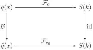
Another natural protocol is a slow, adiabatic change of the coupling parameter c. In the quantum realm, under adiabatic changes the eigenstates of the initial Hamiltonian are natu-rally mapped to those of the final Hamiltonian, whereby all natural conserved quantities (the energy, the number of particles, the asymptotic momenta, etc.) are unchanged. In the classical re-interpretation, the scattering data play the role of these conserved quantities. Hence, one considers the dual quenchprotocol: a quench with respect to the scattering data. The scatter-ing dataS(k), associated to a fieldq(x) for the NLSE with couplingc, is kept fixed, and we ask about the field ˜q(x) having the same scattering dataS(k) but under the NLSE with couplingc0.
This is represented on Figure2and the map Bcaptures the effect of this dual quench protocol.
q(x) Fc ✲ S(k)
˜ q(x)
B
❄
Fc0 ✲
S(k) id
[image:22.595.221.377.524.609.2]❄
Figure 2: The dual quench, keeping the scattering data fixed.
Following the idea coming from the quantum picture, we would expect the mapBto represent the result, in the limitt→ ∞, of the adiabatic protocol wherebyq(x) is firstbackwardevolved un-til time−tunder the NLSE with couplingc, thenforwardevolved back to time 0 under the NLSE with a slowly varying coupling fromc(at time−t) toc0(at time 0). This is the classical analogue
of the quantum scattering map for this adiabatic process, limt→∞Pexp h
−iR−0tds Hc(s) i
eiHct
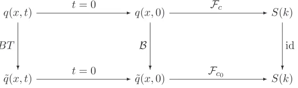
It is well known that B¨acklund transformations play a distinguished role in the theory of integrable PDEs and it is natural to ask whether or not the mapB can correspond to a certain B¨acklund transformation (BT) takingq(x) to ˜q(x). It is natural to reinstate the time dependence as B¨acklund transformations map solutions of a PDE to solutions of a (possibly different) PDE. This question then amounts to showing that the map B on Figure 2 can be seen as the t = 0 restriction of a B¨acklund transformation (BT), see Figure 3.
q(x, t) t= 0 ✲ q(x,0) Fc ✲ S(k)
˜ q(x, t) BT
❄
t= 0
✲ q(x,˜ 0)
B
❄
Fc0 ✲
S(k) id
[image:23.595.154.449.206.293.2]❄
Figure 3: The dual quench as a B¨acklund transformation.
If always true for any value of the quench, it would imply that quenches with respect to the scattering data are of a very special nature: all the resulting fields ˜q(x) are in the orbit of the initial condition q(x) under the action of the group of B¨acklund transformations4. In that case, it would be interesting to obtain an explicit characterization of these transformations in terms of known BT’s and if possible, a formula relating ˜q(x, t) to q(x, t). Note that the crux of the matter here is not to find ˜q since the inverse scattering method tells us how to do this, by applying the inverse transformF−1
c0 to the scattering data S(k). The question is whether or
not the obtained solution ˜q(x, t) can always be seen as an explicit BT of q(x, t) for allt≥0, in which case the question is answered in particular att= 0.
Beyond its interest in terms of adiabatic changes, this question may also shed light on the original quench problem. Indeed, the map B and the quench mapQc,c0 are related as follows:
Fc0B=Qc,c0Fc0. (6.1)
This is an intertwining equation where the intertwiner is the direct transformFc0 of the inverse
scattering method. Hence, knowing B provides us with a formal representation of the quench map as
Qc =Fc0B F
−1
c0 . (6.2)
In general, in the NLSE, we note that the interpretation of B as a BT is either a trivial problem or is very difficult. In the rest of this Section, we present some results towards the answer in some difficult cases. As for the trivial answer, remark that in the rapidly decreasing case, for a quench preserving the nature of the systemi.e. cc0 ∈R, thenBis simply a rescaling
˜
q(x,0) = c c0
q(x,0), (6.3)
which is compatible with the time evolution. So indeed, B can be seen as the t= 0 restriction of the simplest BT
˜
q(x, t) = c c0
q(x, t). (6.4)
4Indeed, it is known that B¨acklund transformations form a group acting on solutions of integrable PDEs, see
In all other cases, this simple answer does not hold. Indeed, in the focusing to defocusing case (or vice versa), c
c0 ∈ i
R and the previous rescaling is not compatible with the time evolution
prescribed by NLSE. To see this, note that ifc=iβ,c0=β0 withβ, β0 ∈Rthen
i∂tq˜+∂2xq˜−2c20|q˜|2q˜= 0, (6.5)
becomes
i∂tq+∂x2q−2β2|q|2q = 0, (6.6)
while it should be i∂tq+∂2xq+ 2β2|q|2q = 0. In the finite density case, things are even more
complicated. Even for a quench preserving the focusing or defocusing nature of the equation of motion, the rescaling alters the boundary conditions and so is not compatible with the prescribed system.
Remark that for integer values of the quench and for a corresponding very specific choice of initial conditions, we see from the three explicit examples treated previously that the net effect on the scattering data is simply to change the number of zeros in the spectral functiona(k), while maintaining its rational form and the reflectionless propertyb(k) = 0. Using6.1, this translates into a mapBwhose effect is to change accordingly the fixed-cscattering data associated toq(x). As we recall below in our short review on BTs, such an effect is easily implemented by using a special type of BT that can add (or remove) exactly one zero in the spectral function a(k) and keep b(k) = 0. These BTs are well-known and their “real” counterpart on q(x, t) can be written explicitely. Combined with the observation that generic scattering data are completely determined by these zeros and the radiative part corresponding to the continuous spectrum of the auxiliary problem, this gives us a strategy to characterize ˜q in terms ofq via a set of special BTs and a transformation taking care of the radiative part. It turns out that the latter is well encoded in the so-called Rosales solution of NLSE [51] which has a simple interpretation in terms of the usual Gelfand-Levitan-Marchenko approach to the inverse part of the inverse scattering method. In the rest of this Section, we present the aforementioned two ingredients (special BT’s and Rosales solution) and then combine them to obtain some more understanding of the map
B in the generic case.
6.1 Review of B¨acklund transformations
The general notion of B¨acklund transformations in integrable PDEs, that is of a transformation q 7→ q˜ such that ˜q is a solution of PDE2 if q is a solution of PDE1 and vice versa, is closely related to the theory of the so-called Darboux matrices which acts on the wavefunctions of the associated auxiliary problem encoding the involved PDEs. That is why in the context of integrable PDEs, they are sometimes called Darboux-B¨acklund transformations. The theory is well-known and we follow here the book [58]. We are interested in the case where PDE1 and PDE2 are the same equation i.e. the NLSE in our case. We focus on the rapidly decreasing case here to present the ideas and comment on an extension to the finite density case at the end of this Section. Let us recall the main steps to obtain a transformation that precisely adds or remove one simple zero to the scattering coefficient a(k) while keepingb(k) unchanged.
The idea is to construct a matrix Dsuch that Ψ =e DΨD0 is solution of (
e
Ψx= (−ikσ3+fW(x, t))Ψe, e
Ψt= (−2ik2σ3+Pe(x, t, k))Ψe,
when Ψ is solution of
(
Ψx= (−ikσ3+W(x, t))Ψ,
Ψt= (−2ik2σ3+P(x, t, k))Ψ,
(6.8)
as before. The constant matrixD0 is used to preserve the normalisation of Ψ. One immediately
obtains the equations
(−ikσ3+fW)D=D(−ikσ3+W) +Dx, (6.9)
(−2ik2σ3+Pe)D=D(−2ik2σ3+P) +Dt. (6.10)
Let us choose
D(x, t, k) =k1I−Σ(x, t). (6.11)
Then, the new potential Wf(x, t) is readily obtained from the old one W(x, t) by
f
W =W +i[σ3,Σ]. (6.12)
The effect on the scattering data is given by
e
S(k) = (D−)−1S(k)D+ (6.13)
where the new scattering matrix is defined by
e
Ψ+(x, k) =Ψe−(x, k)S(k)e , (6.14)
and
D±=
lim
x→±∞D −1
. (6.15)
It remains to find an appropriate Σ. It is shown in [58] that one can choose
Σ =HΛH−1, Λ =
k0 0
0 k∗
0
, (6.16)
where Imk0 >0 andH is made of two column vectors that are solution of (6.8) fork=k0 and
k=k0∗. It can be chosen as
H =
α(x, t, k0) β∗(x, t, k0)
c
c∗β(x, t, k0) α∗(x, t, k0)
, (6.17)
where
α(x, t, k0)
c
c∗β(x, t, k0)
is solution of (6.8) for k=k0. In this case, we obtain
Σ = 1
1− c c∗|σ|2
k0−k0∗cc∗|σ|2 (k0∗−k0)σ∗ ǫ(k0−k∗0)σ k0∗−k0cc∗|σ|2
, σ = β
α. (6.18)
Let us denote
Ψ−= (R,R)eb −ikxσ3, Ψ+= (L, L)eb −ikxσ3. (6.19)
Given the analytic properties of Ψ±, a candidate forα and β is
α(x, t, k0)
c
c∗β(x, t, k0)
=Re−ik0x−µLeik0x, (6.20)
1. Ifk0 is not a zero of a(k) then lim
x→∞σ = 0 and limx→−∞σ=∞ so that
D+ =
1
k−k0 0
0 k−1k∗
0
!
, D− =
1
k−k∗
0 0
0 k−1k0
!
. (6.21)
2. If k0 is already a zero of a(k) and we choose µ to be different from the corresponding
norming constant then lim
x→∞σ=∞ and limx→−∞σ= 0 so that
D+ =
1
k−k∗
0 0
0 k−1k
0
!
, D− =
1
k−k0 0
0 k−1k∗
0
!
. (6.22)
Inserting in (6.13), we get the effect on the scattering data as desired. In both cases,b(k) is untouched: ˜b(k) =b(k). In the first, case ˜a(k) = k−k0
k−k∗
0a(k) and the net effect of the
transforma-tion is to add a simple zero in the upper half-plane toa(k). In the second case, ˜a(k) = k−k∗0
k−k0a(k),
and the net effect is to remove the simple zerok0 ofa(k). We can also extract the corresponding
transformation of the solution q(x, t) in real space, which was our motivation for introducing these transformations in this Section,
˜
q =q− 2i(k
∗ 0−k0)
c(1− c c∗|σ|2)
σ∗ (6.23)
6.2 Review of the Rosales solution
In [51], Rosales proposed a direct solution method for certain integrable nonlinear PDEs based on a series expansion approach. Writing
q(x, t) =
∞ X
n=1
εnψn(x, t), (6.24)
with ψn → 0 as |x| → ∞, and inserting in NLSE, Rosales reduces the problem to finding a
function Φn(k1, . . . , kn) by making the ansatz
ψn(x, t) =
Z
Cn
Φn(k1, . . . , kn)eiΩndλ(k1). . . dλ(kn). (6.25)
Here dλis a measure over Cand5
Ωn= n
X
j=1
−kjx+ (−1)jkj2t
. (6.26)
The final results reads
q(x, t) =ε
∞ X
n=0
(−c2ε2)n
Z
C2n+1
eiΩ2n+1
2n
Q
j=1
(kj+kj+1)
n
Y
j=0
dλ(k2j+1)
n
Y
j=1
dµ(k2j) (6.27)
5Note that we took the convention−
withdµ∗(−k∗) =dλ(k). This special relation comes from the fact that both q and q∗ appear in
NLSE. Rosales then shows that this series can be resummed for not necessarily small values ofε and in particular one can setε= 1. The point is that the entire content of the inverse scattering method can be encapculated in the choice of the measure. For instance, by choosing a purely discrete measure, one can reproduce the well-known solitons solutions of the inverse scattering method. In the present context, we want to make use of the Rosales resolution in the opposite situation where only the continuous spectrum is present. This gives us a series representation of the so-called radiative solution of NLSE. This corresponds to choosing a continuous measure of the formdλ(k) =βρ(k)dk for some function ρ with support on R and some constantβ. An
interesting aspect of Rosales’s approach is that one can perform a resummation of the series representation. In general, the resummation is rather formal but Rosales gives some conditions under which it is rigorously meaningful. It is beyond the scope of this paper to investigate these precise conditions. We will explain below how this gives us a means to discuss the issue at hand: the quench from a focusing to a defocusing system (or vice versa).
We now show how the Rosales expansion is related to the standard Gelfand-Levitan-Marchenko (GLM) approach to the inverse scattering method. Although this is probably known to the ex-perts, we have not found the explicit connection anywhere, except in [59]. So we provide the main steps in what follows. The Neumann series approach to the solution of the GLM equation in the case where the scattering dataa(k) has no zeros produces exactly a Rosales type solution, for a special case of the measuredλ(k). The interpretation ofρ(k) in this context is clear: it is the reflection coefficient ba((kk)). The constant β is related to the parameter c (see (6.37) below). We recall the main steps of the GLM method in the rapidly decaying case, referring to [50] for details, and then present the Neumann series solution of the GLM equations to make contact with the Rosales solution.
The starting point of the GLM method is to introduce a kernel K via the relation
Ψ−(x, k) =e−ikxσ3+
Z x
−∞
ds K(x, s)e−iksσ3, (6.28)
with
K(x, y) =
K∗
1(x, y) K2(x, y)
c
c∗K2∗(x, y) K1(x, y)
. (6.29)
Inserting these expressions into (2.9) leads to partial differential equations for K1 et K2 for
which existence and uniqueness of solutions have been established in the case of NLSE, see for instance [50] and references therein. The important relation to reconstructq reads
cq(x,0) =K2(x, x). (6.30)
Indeed, it can be shown that the kernel element K2 can in principle be obtained from the
scattering data via the GLM equation, for y≤x,
K2(x, y) =−F(x+y) +
c c∗
ZZ x
−∞
ds1ds2 F∗(s1+s2)K(x, s1)F(s2+y) (6.31)
where
F(x) =
Z
C
dk 2π
b(k) a(k)e
is a (Fourier) transform of the reflection coefficientρ(k), ratio of the scattering coefficient a(k) and b(k). The contourC goes from −∞+i0 to∞+i0 above all the zeros of a(k) in the upper half-plane. In the case of interest for us, we assume that a(k) has no zeros (as we can always remove them with the BTs discussed above) and we can deform the contour down to the real line (from above). We iterate the equation to form the Neumann solution forK2,
K2(x, x) =−F(2x)− ∞ X
n=1 c
c∗ nZ x
−∞
. . .
Z x
−∞
d2nzF∗(z1+z2). . . F∗(z2n−1+z2n)
×F(x+z2n−1)F(z2n+z2n−3). . . F(z4+z1)F(z2+x). (6.33)
Using (6.32), we can perform the integrals overzj which involve integrals of the form
Z x
−∞
dz ei(k∗2j−k2j±1)z = e
i(k∗
2j−k2j±1)x
i(k∗
2j−k2j±1)
. (6.34)
In the limit where the imaginary part ofkj tends to 0 from above, this yields the usual
prescrip-tion
Z x
−∞
dz ei(k2j−k2j±1)z= e
i(k2j−k2j±1)x
i(k2j−k2j±1−i0)
. (6.35)
Hence we obtain,
q(x,0) =−1
c ∞ X n=0 −c c∗ nZ
R2n+1
d2n+1k
(2π)2n+1
n
Y
j=1
ρ∗(−k2j) nY+1
j=1
ρ(k2j−1)
e−2
i
2nP+1
j=1
kjx 2n
Q
j=1
(kj +kj+1+i0)
, (6.36)
We see that this expression is a particular case of the Rosales expansion if we choose the measure dλ(k) to be of the form
dλ(k) =−1
εcρ(k) dk
2π, (6.37)
where we recall thatρ(k) = ba((kk)), with the understanding that it is supported on the real line. Let us just note that the factor 2 in the exponential term comes from the choice of normalisation in kin the auxiliary problem, leading to an extra factor 2 in the corresponding Fourier transform, as already noted in Section 4.1when dealing with the quench to the free case.
This observation allows us to take advantage of the result obtained in general by Rosales concerning the resummation of the series representation for the solution. The idea is to extend basic vector and matrix representations that would occur in the case of a discrete measure over a finite number of points (the case of a pure multisoliton solution) to functions and operator kernels in order to deal with the purely continuous case that concerns us. Thus, let us define the function
f(k) =e−i(kx+k2t), (6.38)
and the operator O acting on appropriate functions g(k) as
(Og)(k) = 1
2iπ
Z
R
f∗(k)f(ℓ)