A Generative Design Technique for Exploring Shape
Variations
Shahroz Khana,∗, Muhammad Junaid Awana
aBrainlabs Software, Taxila, Pakistan DOI.
Abstract
Because innovative and creative design is essential to a successful product, this
work brings the benefits of generative design in the conceptual phase of the
product development process so that designers/engineers can effectively explore
and create ingenious designs and make better design decisions. We proposed
a state-of-the-art generative design technique (GDT), calledSpace-filling-GDT
(Sf-GDT), for the creation of innovative designs. The proposed Sf-GDT has the
ability to create variant optimal design alternatives for a given computer-aided
design (CAD) model. An effective GDT should generate design alternatives that
cover the entire design space. Toward that end, the criterion of space-filling is
utilized, which uniformly distribute designs in the design space thereby giving
a designer a better understanding of possible design options. To avoid creating
similar designs, a weighted grid search approach is developed and integrated
into the Sf-GDT. One of the core contributions of this work lies in the ability
of Sf-GDT to explore hybrid design spaces consisting of both continuous and
discrete parameters either with or without geometric constraints. A
parameter-free optimization technique, called Jaya algorithm, is integrated into the Sf-GDT
to generate optimal designs. Three different design parameterization and space
formulation strategies; explicit, interactive, and autonomous, are proposed to
set up a promising search region(s) for optimization. Two user interfaces; a
∗Corresponding author
web-based and a Windows-based, are also developed to utilize Sf-GDT with
the existing CAD software having parametric design abilities. Based on the
experiments in this study, Sf-GDT can generate creative design alternatives for
a given model and outperforms existing state-of-the-art techniques.
Keywords: Generative Design, Computer-Aided Design, Parametric Design,
Space-filling Design, Jaya Algorithm
1. Introduction
Engineering or industrial product design is a complex process in which a
de-sign arrives at its final form after passing through a series of dede-sign phases. The
conceptual phase is an initial and important component of these phases; it is
rec-ognized as a foundational step in any product development process. This phase
5
can be complex and time-consuming if the appearance of the product under
consideration is valuable to its target customers. To select an appealing design,
designers often develop a number of design alternatives using two-dimensional
(2D) sketches. However, the formulation of these alternatives is a critical and
time-consuming task, especially for novice designers. To create these
alterna-10
tives, designers have to develop and explore the entire design space effectively
within a product’s design requirements or the customer’s preferences.
Exploration of design alternatives is recognized as a major characteristic
of the conceptual design phase [1, 2]. Pahl et al. [3] categorized the
concep-tual phase into two sub-phases. In the first sub-phase, design alternatives are
15
formalized based on the design requirements. In the second phase, these
alter-natives are ranked based on a preliminary analysis to select a potential design.
Computer-aided design (CAD) is rarely used during this phase; it is primarily
utilized later to analyze, validate, and fabricate the design [4]. For the most
part, design engineers convert a design selected at the conceptual phase into a
20
CAD model when they explore a narrow design space in order to analyze the
performance of the design.
sim-ulation, and parametric design techniques, the role of computers in the field of
design is changing. In comparison to traditional CAD modeling techniques,
25
these new techniques allow designers and engineers to iterate through a large
number of design alternatives [5]. Generative design systems use these
tech-niques to provide a promising way to explore design space to create alternative
designs based on the specific performance objective defined by a user. A
typi-cal generative design system takes a problem definition as input and produce a
30
single or set of optimal solutions for a given problem. Commercially available
generative design systems, such as Altair’s OptiStruct, solidThinking’s Inspire,
Siemen’s Frustum, and efiForm [6], etc., are based on the topology optimization
techniques [7]. These techniques are the mathematical methods that optimize a
layout of material distribution within a predefined design space. Mostly, in these
35
systems, the objective is to maximize/minimize compliance, the temperature at
a certain point or globally, or minimize weight under volume, stress or
displace-ment constraints. Typically, a generative system involves three steps to set up a
problem. First, design engineer transforms 2D sketches into a three-dimensional
(3D) CAD model. Then, various constraints and properties are defined based
40
on the design specifications. Later, the design engineer executes generations to
obtain a single or multiple optimization solutions. Different researchers have
de-veloped GDTs to create architectural structures [8], site layouts [9], and energy
efficient [10] and eco-friendly building designs [11]. However, few studies[12, 4]
have investigated how to create generative systems to explore designs based on
45
their external form appearance.
Therefore, it is beneficial to develop a system that can automatically generate
a variety of unique design alternatives for the outer form of a product based on
its design requirements. The prime objective of this study is to develop a GDT
that can effectively explore a design space and generate optimal aesthetically
50
convincing design alternatives for a product at the conceptual phase of the
design process. To develop the proposed technique, the following points were
1. Have an effective search and generation strategy to generate optimum
design alternatives.
55
2. Be able to autonomously set up a viable design space for a given model.
3. Be able to work with both continuous and discrete design parameters.
4. Be able to create uniformly distributed and variant designs from the entire
design space.
5. Have the ability to effectively explore both constrained and unconstrained
60
design spaces.
By considering the points mentioned above, the present study proposes a
new generative design technique,Space-filling-GDT (Sf-GDT). Sf-GDT has the
ability to generate variant optimal designs. However, the decision on the
selec-tion of appropriate design parameters and setting a suitable design space for a
65
given problem is critical. Therefore, Sf-GDT provides different space
formula-tion strategies for the users to obtain optimal designs. Generative formulaformula-tion of
designs is a high-dimensional constrained optimization problem as there are
gen-erally a high number of design parameters and geometric constraints. Therefore,
there is a need for a simple yet effective optimization approach that can search
70
different optimum designs. Among many well-known optimization techniques,
genetic algorithms have been widely used in generative systems. However, the
performance of the genetic algorithms extensively depends on the selection of
tuning parameters [13] and the proper tuning of these parameters requires an
entirely different set of expertise, which most designers do not possess [12]. For
75
this reason, we selected a newly proposed simple, effective, and parameter-free
optimization approach called Jaya algorithm [14].
To generateN optimum design alternatives, the user first parameterizes the
given CAD model and define a viable design space based on any of the three
different proposed space formulation techniques. Within the defined design
80
space, Sf-GDT randomly generates an initial population of solutions/designs,
which consists of a further N subpopulations, one for each design alternative.
subpopulation to converge the initial solutions to the optimum position in the
design space while minimizing a cost/objective function, which ensures uniform
85
and diverse design exploration. A weighted grid search approach is proposed,
which enables Sf-GDT to maintain diversity between designs. Sf-GDT has also
the ability to explore design space by synthesizing the design with different style
forms, which can be implemented as discrete design parameters. To generate
designs from the constraint spaces, Sf-GDT uses Deb’s heuristic constrained
90
handling rules [15]. Figure 1 illustrates the outcome of the proposed technique.
Following major contributions are made to Sf-GDT to enhance its ability for
optimal creation of designs.
1. The search strategy of Jaya algorithm is extended to generateN optimal
designs.
95
2. A weighted grid search technique is embedded in Sf-GDT to maintain
diversity between designs.
3. The ability of Sf-GDT is enhanced to explore hybrid design spaces
con-sisting of continuous and discrete design parameters.
4. Different design parameterization and space formulation strategies are
pro-100
posed for an effective creation of design space.
5. Deb’s [15] heuristic constraint handling rules are applied to generate
de-signs in constrained spaces.
6. A web-based and Windows-based user interfaces are developed to utilize
Sf-GDT with existing CAD software.
[image:5.612.203.404.553.641.2]105
The remainder of this paper is organized as follows: Section 2 gives a
com-prehensive review of the relevant literature. Section 3 discusses the proposed
approach to generating new designs. The numerical results of the proposed
technique are given in Section 4. Section 5 describes the usage of the proposed
technique with existing CAD software. Concluding remarks and opportunities
110
for future work are presented in Section 6.
2. Related works
The proposed technique is inspired by the prior research in generative and
space-filling design techniques and is based on Jaya algorithm. Below, we discuss
some previous works done by different researchers in these fields.
115
2.1. Jaya Algorithm
Most of the well-known meta-heuristic optimization techniques require
algorithm-specific parameters and proper tuning of these parameters is a critical factor,
which affects their performance [13]. For example, the genetic algorithm uses
selection operator, mutation and crossover probability; particle swarm
optimiza-120
tion uses inertia weight, cognitive and social parameters; artificial bee colony
uses the number of onlooker bees, scout bees, and employed bees. The Jaya
algo-rithm does not require tuning of specific parameters except common controlling
parameters like population size and a number of generations. This simplicity
and tuning free nature of the Jaya algorithm make it suitable for generative
125
design systems.
The optimization process in Jaya starts by randomly generating a population
Pof initial solutions for a given sizeswithin then−dimensionaldefined design
space. In order to achieve an optimum solution during the search, the algorithm
always tries to move towards the best solution and moves away from the worst
130
solution. Suppose for a specific problem there arennumber of design parameters
the value of thejth parameter for the kth solution during the ith iteration is
represented asXj,k,i, then this value is updated according to Equation (1).
Xj,k,i0 =Xj,k,i+r1,k,i(Xj,best,i− |Xj,k,i|)−r2,k,i(Xj,worst,i− |Xj,k,i|) (1)
Xj,best,i andXj,worst,iare the updated values of the parameterjfor the best
135
and worst solutions, respectively. Xj,k,i0 is the updated value ofXj,k,i, andr1,k,i
andr2,k,i are the two random numbers in the range [0,1]. At the end of each
iterationiifXj,k,i0 is better thanXj,k,ithen it is accepted otherwise rejected.
Several improvements have also been made on the Jaya algorithm in order
to improve its performance and to expend its application in different fields. For
140
example, Huang and Wang [16] introduced an elite opposition-based Jaya
algo-rithm called EO-Jaya. EO-Jaya is a swarm intelligence based algoalgo-rithm with
no specific parameters to tune its performance. The elite opposition learning
strategy was incorporated into EO-Jaya’s solution updating phase, which
en-hances the solution diversity. A hybrid parallel Jaya algorithm for a multi-core
145
environment called HHCP was developed by Michailidis [17]. HHCP Jaya has
a hierarchical cooperation search mechanism to solve large-scale global
opti-mization problems. Another version of Jaya called SAMP-Jaya algorithm was
introduced by Rao and Saroj [18] for solving the constrained and unconstrained
numerical and engineering optimization problems.
150
Jaya algorithm and its variations have also been implemented to different
fields of science and engineering such as manufacturing [19], classification [20],
power [21], combinatorial optimization [22] and topology optimization of truss
structures [23].
2.2. Generative Design
155
To date, the field of generative design has been passed through the various
advancements for different applications. Several GDTs have been proposed by
different researchers for architectural applications and for the creation of a
applications, here, we discuss some recent studies that are close to the proposed
160
technique.
An exhaustive searched based GDT was proposed by Krish [12] for
creat-ing design alternatives. In which, designs are randomly searched in the design
space and to generate dissimilar designs, the designer defines a threshold value,
which is set on the Euclidean distance, between the generated designs. A major
165
drawback of this technique lies in its exhaustive search strategy, which hinders
designers from exploring and creating optimum design options. A practical
gen-erative design system calledDreamSketch was developed by Kazi et al. [4] to
support generative design at the conceptual phase. In DreamSketch, a user
cre-ates an initial design by sketching and then its alternatives are generated in the
170
sketched context. In order to benefit from DreamSketch, a user requires
pos-sessing digital sketching abilities. A shape sampling technique, similar to ours,
have been proposed by Gunpinar and Gunpinar [24], and Khan and Gunpinar
[25]. However, these techniques lack the ability to work with discrete
param-eters and present no practical approach to design parametrization and design
175
space formulation. Furthermore, the sampling technique of [25] is
computation-ally expensive compared to the proposed technique. A biologiccomputation-ally motivated
algorithm was developed by Runions et al. [26] for the generative creation of
leaf venation patterns. Sousa and Xavier proposed a symmetric-based
genera-tive technique for digital fabrication of geometric shapes like a triangular prism,
180
cuboctahedron, and rhombicuboctahedron, etc.
In literature, techniques like shape grammars [27], shape syntheses [28] and
L-systems [29] have been utilized by researchers to develop generative systems.
Shape grammars are a generative method for creation of design alternatives by
incorporating geometric logics/rules and have been utilized in different
appli-185
cations such as product design [30], architectural design [27], and embroidery
design [31], etc. Despite being its usage for different application, shape
gram-mars’ usage is limited to the industry because of its computational complexity
and difficulty in developing user interfaces [32]. L-systems are a variation of
shape-grammars and has been used for different design problems such as
plex city planning [33] and computer pattern design [34]. L-systems are also
based on the design rules applied in the form of a string. Among these
meth-ods, shape syntheses are preferable for creating a higher design variation of
a given design. However, these techniques can only be employed for creating
variations of existing designs/shapes. In which system is first trained on a large
195
dataset of existing designs/shapes that are then synthesized to create variations.
2.3. Space-filling Design
There is a considerable amount of research that has been done on the
opti-mal selection of space-filling Design of Experiments (DoE). However, most works
done by researchers are proposed for the unconstrained design spaces. The
re-200
search problem becomes more complicated when a selection of designs has to
be performed in a constrained and high-dimensional design space like in the
re-search of this paper. Fuerle and Sienz [35] proposed a method to produce designs
in constrained spaces. However, this method is not feasible for high-dimensional
problems more than 3D. Dragulji´c et al. [36] proposed a CoNcaD algorithm for
205
constructing non-collapsing and space-filling designs for bounded
nonrectangu-lar design spaces. Trosset [37] and Stinstra et al. [38] used maximin criterion
for the construction of space-filling designs in the constrained 10-dimensional
design space. The technique proposed by Trosset [37] and Stinstra et al. [38]
does not guarantee the sampled DoE to be non-collapsing.
210
3. Proposed Technique
This section presents details of the proposed Sf-GDT that explores a design
space to generate N designs. We first outline the core idea behind Sf-GDT
approach and then the ability of Sf-GDT to explore constrained spaces with
continuous and discrete design parameters will be explained.
215
3.1. The Sf-GDT
Basic terminologies are described first in relation to problem setting. A CAD
Each design parameter defines a dimension in the design space. To form the
design space limits, the upper and lower bounds for each design parameter are
220
set. [xlm,j] and [xum,j] represents the lower and upper bounds of the jthdesign
parameter, respectively, wherej = 1,2,3, . . . , n. Therefore, an−dimensional
design space is formed by a set ofn design parameters along with their lower
and upper bounds.
To generate an optimal set of N design alternatives with the appropriate
225
degree of dissimilarity, designs must be uniformly distributed with the maximum
separating distance within then−dimensionaldesign space. Therefore, a cost
function based on the Audze and Eglais [39] technique is utilized, which follows
a physical analogy: Molecules in a space exert repulsive forces on each other
that lead to potential energy in a space. These molecules are in equilibrium in
230
case of minimum potential energy. The analogous potential energy U1(B) for
the creation of the space-filling designs is defined as:
U1(B) =
N−1
X
p=1
N X
q=p+1
1 L2
pq
(2)
where
Lpq= v u u t
n X
j=1
(xp,j−xq,j)2 (3)
Here, Lpq is the distance between the designs p and q, and xp,j and xq,j
are thescaled parameter values for the jth dimension of these designs, which
235
are computed by scaling parameter values between 0 (i.e., lower bound for the
parameter) and 1 (i.e., upper bound for the parameter). The design space
formed from these bounds is called scaled design space. Recall that N is the
number of designs to be generated andn is the number of dimensions in the
design space.
240
The optimization problem for Sf-GDT can be formulated as the
minimiza-tion of U1(B) to generate N optimum solutions (or designs). However,
ini-tial population of individuals to an optimum position. Therefore, the search
strategy of Jaya algorithm has to modify in order to provide N optimum
so-245
lutions. The optimal design creation process of Sf-GDT starts by creating
the random initial population P consisting of N subpopulations (i.e., P =
[(p1)s×n, (p2)s×n, (p3)s×n, . . .(pN)s×n]T). pL = [X1, X2, . . . Xs]T denotes
theLthsubpopulation ofP andL= 1,2,3, . . . , N. Each subpopulation consists
ofssolutions and thesthsolutionX
sis comprised ofndesign parameters (i.e.,
250
Xs= [xs,1, xs,2, . . . xs,n]).
For each solution, there is a subpopulation of sizes, during convergence all
theN subpopulations are guided to their optimum position with Equation (1)
under the consideration of their best and worst solutions. N worst and best
solutions are selected, one from each subpopulation. The best and the worst
255
solutions are the individuals that minimize and maximizes the cost function,
receptively. The cost function is calculated based on the best solutions of the
subpopulations. The division of population P into subpopulations is similar
to [18, 25]. Let B = [B1, B2, . . . , BN] and W = [W1, W2, . . . , WN] are sets of
best and worst solutions, respectively, and BL and WL is the best and worst
260
solution for theLthsubpopulation. For the selection ofN best and worst initial
solutions, there are 2×sN combinations. This means that the cost function
has to be evaluated 2×sN times. For instance, atN = 10 ands= 40 setting,
2×10485760000000000 evaluations of cost function has to be performed for
the selection of B = 10 and W = 10 solutions. This can result in a high
265
computational cost if N or s are assigned to a larger value. Therefore, an
initial-designs-selection strategy is utilized for the selection of N initial worst
and best solutions.
The initial-designs-selection strategy for the selection of N best initial
so-lutions is based on the fact that the best individuals have the ability to select
270
other exceptional individuals from a group. Following the similar analogy, N
is first set to 2 in the cost function, and two individuals of the first two
sub-populations that minimize the cost are selected as best solutions B1 and B2.
solutionB3 from the third subpopulation. This solution is selected under the 275
consideration of the preselected solutions B1 and B2 by setting N = 3. The
selection process is repeated in a similar manner untilN best solutions from the
N number of subpopulations are determined. Similarly, this selection strategy
is utilized to selectN worst solutions, which maximizes the cost function. Note
that this selection strategy checks 2×s2+PN
2 s individuals’ combinations to 280
select each set ofN best and worst initial solutions.
In Sf-GDT, the optimization process in any iteration is completed by
per-forming the N number of sub-iterations, one for each subpopulation. Each
subpopulation moves towards the better position in design space individually
while keeping the best and worst solutions of other subpopulations the same.
285
During optimization, a new position for a solution is found using Equation (1).
LetXk and Xk0 be the current and new positions of a solution in the first
sub-population, respectively. The new position of the solution is accepted if the cost
value ofB0 = [Xk0, B2, . . . , BN] is less thanB = [Xk, B2, . . . , BN]. The bestB
and worstW solutions are updated after each sub-iteration for the
subpopula-290
tion. The best solution is an individual having a minimum cost value (computed
with the best solutions of other subpopulations) among the other solutions in
the same subpopulation. Sub-iterations in other subpopulations are performed
in the same way. An iteration is completed when a sub-iteration for each of the
subpopulation is performed. After Sf-GDT stops the convergence process the
295
best solutions of the subpopulations are regarded as final optimal designs.
Furthermore, the alternatives obtained from Sf-GDT can work as Design
of Experiments (DoE) for physics simulations, which can be run for validation
of designs’ functionality, structural integrity, and usability. DoE are crucial
in physical analyses, which has the major goal of determining which design
300
parameters have more effect on the simulation results. Most analyses are
com-putationally expensive, and running the analysis for collapsing designs and
3.2. Weighted Grid Search Technique
Minimization of U1(B) favors placement of the designs at the maximum 305
separating distance from each other. In the case of high-dimensional design
space, this function itself locates some designs at the boundaries of the design
space [40]. This will result in the violation of a non-collapsing criterion [36] (i.e.,
designs not sharing any parameter values within a specific interval), thereby
generating similar designs.
310
For generative designs, it is desired to spread designs evenly also in the
inner portions of the design space. Therefore, the non-collapsing criterion for
the generated designs should be satisfied as much as possible. A weighted grid
search technique is introduced in order to generate non-collapsing designs in the
design space. A new term,U2(B), is included in the cost function, which is as 315
follows:
U2(B) =α×
N−1
X
p=1
N X
q=p+1
n X
j=1
f(yp,j, yq,j) (4)
f(yp,j, yq,j) =
1 ifyp,j=yq,j
0 otherwise
(5)
where
if xep,j ≤xp,j< xep,j+1 then yp,j=e
if xeq,j ≤xq,j< xeq,j+1 then yq,j =e
(6)
The term U2(B) is based on the degree of violation for the non-collapsing
criterion. Here, α is a user-defined parameter adjusting weight of the U2(B)
term. yp,j and yq,j in Equation (4) are the corresponding integer coordinate
320
values forxp,jandxq,j in thejthdimension, respectively. To calculateyp,jand
yq,j the range of each design parameter is partitioned into N equal intervals
(levels) as follows: [xlm,j =x1m,j, xm,j2 , . . . , xNm,j =xum,j] and an integer
on these integer values, the piecewise functionf in Equation (5) decides if the
325
designspandqare collapsing or non-collapsing.
Maximum value for this term can ben× N2
. N2represents the
combina-tions between designs, which is as follows: N2
= N!
2!(N−2)!. Setting the
param-eterαto small values will lead to semi non-collapsing designs and larger values
will produce more non-collapsing designs. The cost function U(B), which is
330
given in Equation (7), have to minimize to create space-filling and non-collapsing
designs. This function is overall composed of a parameter α, andU1(B) and
U2(B) for space-filling and non-collapsing criteria, receptively. Algorithm 1
summarizes the step-wise procedure of Sf-GDT.
M inimize U(B) = N−1
X
p=1
N X
q=p+1
1 L2
pq
+ α×
N−1
X
p=1
N X
q=p+1
n X
j=1
f(yp,j, yq,j) (7)
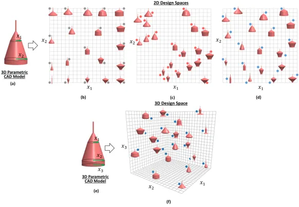
Figure 2 (a) shows a 3D CAD model parameterized with two design
param-335
eters x1 and x2. The design parameter and their parametric ranges ([xl1] ≤
x1 ≤[xu1] and [xl2] ≤ x2 ≤[xu2]) forms a 2D design space. 20 design
alterna-tives for this CAD model are created using the proposed Sf-GDT under the
space-filling criterion (Equation 2), Non-collapsing criterion (Equation 4) and
combined space-filling and non-collapsing criteria (Equation 7), which are shown
340
in Figure 2 (b), (c) and (d), respectively. It should be noted that each point/dot
in the Figure 2 represents a position of a design in the design space. In Figure
2 (a), it can be seen that the design alternatives are spread evenly in the design
space, therefore, space-filling designs can be obtained using Sf-GDT. However,
in this case, there are more designs are the boundary of the design. Therefore,
345
exploration performed only based on this criterion may not produce satisfactory
designs because during space exploration designer desires to obtain designs that
also evenly covers the inners regions of the design spaces. Furthermore, the
design alternatives in Figure 2 (c) are created with the only non-collapsing
cri-terion and has resulted in designs with the poor space-filling property. It can be
350
observed in the Figure 2 (c) that the better space exploration is achieved when
when space exploration is performed using the Equation 7, which involves both
space-filling and non-collapsing criterion). Later, the 3D CAD model in Figure
2 (e) is parameterize with design parametersx1, x2 andx3. Here, these three 355
design parameters form a 3D design space. 20 design alternatives are created
in the 3D space using the Sf-GDT (see Figure 2 (f)). Again, the points in this
[image:15.612.159.450.238.440.2]space represent the positions of the 20 design alternatives.
Figure 2: Design alternatives for a 3D CAD model with two design parameters (a) are obtained
in 2D spaces considering; (b) only space-filling criterion, (c) only non-collapsing criterion, and
both space-filling and non-collapsing criteria using Sf-GDT (d). Design alternatives for the
same CAD model with three parameters (e) are generated in 3D design space using Sf-GDT
while considering both space-filling and non-collapsing criteria (f).
3.3. Sf-GDT for Discrete Parameters
Sf-GDT also gives the ability to the designer to explore design space by
360
synthesizing the design with different ”style” profiles (e.g., round, triangular,
and rectangular, etc). The designer can add an option for variable base styles
that can be implemented as discrete design parameters. Sf-GDT is customized
in the following way in order to be employed for the discrete design parameters.
Suppose, an integer value (round→1, rectangular→2, and triangle→3) is
Algorithm 1The pseudo-code of Sf-GDT
1: Create an input CAD model and parameterize it with n design parameters
(x1, x2, . . . , xn).
2: Initialize the number of parameters (n), parameter ranges, number of design to be
created (N), subpopulation size (p) and parameterα.
3: Randomly create an initial populationP of feasible solutions/designs within the
parametric ranges consisting of N subpopulations (pL)s×n of sizes, where 1 ≤
L≤N.
4: Obtain set ofN initial best (B) and worst (W) designs, one from each
subpopu-lation based on the initial-designs-selection strategy.
B= [B1, B2, . . . , BN],W = [W1, W2, . . . , WN]
5: whiletermination criterion is not satisfieddo
6: forL= 1 toN do
7: fork= 1 tos do
8: Update the designXk of (pL)s×n using Equation 1 based on theBL and
WLand obtain an updated/new designXk0.
9: Calculate the cost value U(B0) and U(B) using Equation 7 for B =
[X10, B2, . . . , BN] andB= [X1, B2, . . . , BN].
10: if U(B0)< U(B)then
11: Accept the designXk.0
12: else
13: Accept the designXk.
14: end if
15: end for
16: Obtain the updated (pL)s×n, which is (p 0 L)s×n.
17: Find the new bestBL0 and worstW
0
Lsolutions from (p 0 L)s×j.
18: ReplaceBLandWLwithB0LandW
0
Lin the initial set (B= [B 0
1, B2, . . . , BN],
B= [W10, W2, . . . , WN]).
19: end for
20: end while
21: FinalN optimal designs are obtained.
assigned to each of three styles. Letxp,dbe thedthdiscrete parameter of design
pcontaining t styles and [xlp,d] and [xup,d] are the lower and upper bounds for
xp,d, respectively. In the above case, t = 3, [xlp,d] = 1 and [xup,d] = 3. Instead
t number of styles. Now, the range of xp,d is divided into t equal number of
370
intervals as follows: [xlp,d=x1p,d, xp,d2 , . . . , xtp,d=xup,d]. After Sf-GDT converge,
all the design parameters, includingxp,d, of each design consists of continuous
values. The parameter xp,d contains the style profiles in the form of discrete
values and required to be converted to discrete values. Otherwise, no decision
can be made on the selection of the style shape. Therefore, after generatingN
375
designs, continuous values ofxp,dfor each design will be converted into discrete
values by using Equation (8).
if xrp,d≤xp,d< x r+1
p,d then xp,d=r (8)
Here, rin an integer number ranging from 1 tot.
3.4. Generation of Design from Constrained Spaces
The design space consists of feasible and infeasible regions in the presence
380
of geometric constraints. Feasible regions consist of feasible designs that satisfy
the predefined constraints. Infeasible designs are located in the infeasible
re-gions. There are different types of constraint handling techniques are available
in the literature, such as the incorporation of static penalties, dynamic
penal-ties, adaptive penalties etc. In this study, Deb’s heuristic constrained handling
385
method [15] is adopted in order to avoid Sf-GDT from selecting designs from
constrained spaces. Deb’s method uses a tournament selection operator in which
two solutions are selected and compared with each other. A designpis said to
be constrained-dominate other design q if any of the following heuristic rules
are true:
390
1. Designpis feasible and designqis not.
2. Designs p and q both are infeasible but design p violate less number of
constraints.
3. Designs p and q both are feasible but design p has better cost function
value.
If design p constrained-dominate design q then design p is selected. This
domination is checked at the end of each sub-iteration. There can be the case
when both designs,p and q, are infeasible and have the same number of
con-straint violations then the design with better cost value is selected. In case of
constraint space, Sf-GDT generates an initial population P consisting of only
400
feasible solutions. So, during the selection of the initial best and worst solutions,
the initial-designs-selection strategy does not have to check these constrained
handling rules.
3.5. Design Parameterization
An effective design parameterization of a CAD model is required to create
405
variant designs. All the important features of the design should be
parameter-ized with the appropriate number of parameters. However, a decision on the
suitable set of parameters is a critical step in the parametrization, which
re-quires the strong understanding of the design requirement and key attributes.
There are different techniques available in the literature on how to form a
well-410
structured parametric model [41]. A well-structured model can enable the
de-signer to create a variety of design alternatives within its design requirement
than a poorly structured model. The high number of design parameters may
not keep the original form of the design. As mostly designers desire to keep the
common underlying structure of the model while generating its alternatives. On
415
the other hand, less number of parameters can narrow down the design space
and larger variation of designs may not be achieved. Therefore, the decision on
the selection of appropriate design parameters should be carefully made.
One strategy, which the designer can follow, is to first detect the important
features of a given model and then these features can be parametrized with
420
a relatively higher number of parameters and designs can be generated with
these parameters. Later, after some trials, the designer can detect quixotic
parameters and eliminate them by directly modifying the CAD model. Such
capability of the generative design system is recognized as ’designerly’ method,
which allows designers to modify the model under consideration and use its
generative capabilities at any phase of the design process [12]. After exploring
the designs based on the important features, later, if required, design space can
be explored based on its nominal features.
3.6. Formulation of design space
As stated before, the design space for any CAD model is formed by the
430
number of the design parameters and their bounds. The dimensionality of the
design space depends on the number of design parameter used to define the CAD
model and the limits of the design space are set by defining the upper and lower
bounds for each design parameter. However, formulation of a suitable design
space is a decisive task as the performance of a technique in term of creating
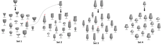
435
better design alternatives mainly depends on it. Setting up the design space
should be carefully done in order to achieve the maximum performance of the
Sf-GDT and should have sufficient high potential region. If design space is too
narrow then Sf-GDT will result in the creation of similar/same designs. On the
other hand, a vast design space can result in the waste of computational effort
440
in exploring undesirable regions of the design space. Typically, a design space is
set up by defining the upper and lower bounds of the design parameters. Where
each parameter represents a dimension in the design space. Defining the upper
and lowers bounds usually done based on the initial design specifications and
designers’ understanding of the design.
445
In Sf-GDT, design space formulation can happen in three different way;
explicit formulation, autonomous formulation, and interactive formulation.
Explicit Formulation: The explicit formulation of the design space
hap-pens when the design specifications are known at the conceptual stage and based
on these specifications the designer limits the space.
450
Autonomous Formulation: The autonomous formulation helps to coarsely
form the design space as a percentage of the initial parameter values of the
de-sign. This formulation happens when no primary understanding of the design
specifications are available in the conceptual phase. The autonomous
formula-tion gives a good initial guess of suitable space limits. With this formulaformula-tion,
the designer can first inadequately build up an initial map of promising regions
of the design space and then explore designs in that space. Afterward, the
de-signer can further reform the design space based on the previous exploration
results. There can be some infeasible designs in the autonomously formalized
space, but this can be overridden by implementing geometric constraints.
[image:20.612.175.433.225.299.2]460
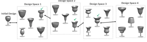
Figure 3: Interactive formulation of design space.
Interactive Formulation: In the interactive formulation of the design
space, the designer creates multiple spaces and gradually proceeds to a final
design. First, the designer can autonomously form an initial design space around
the given CAD model and creates designs in this space. Afterward, the designer
can select a design and then formalize an autonomous space around that design.
465
In this way, the designer can interactively proceed by selecting designs and
forming the design spaces until he/she achieves a final desired design. For
example, Figure 3 gives the illustration of the interactive formulation of the
design space. In which initial space (design space 1) is formed around the
initial design. A design (marked in green) is selected from this space and then
470
a new space (design space 2) is formed around the previously selected design.
This process continues until the final design is achieved. During selection, if the
designer selects more than one design, then a new design space is created around
the centroid of the selected designs. The designer can also refine or shrinks the
space after each interaction as he/she approaches the final design. Once the
475
final design is selected then, if desired, it can be further modified easily due to
4. Results and Discussion
In this section, we first demonstrated a step-wise procedure for implementing
GDT on a simple 3D CAD model and then discuss the performance of
Sf-480
GDT for different test models and settings. The proposed technique has also
been compared with the existing state-of-the-art techniques.
4.1. Implementation of the Sf-GDT
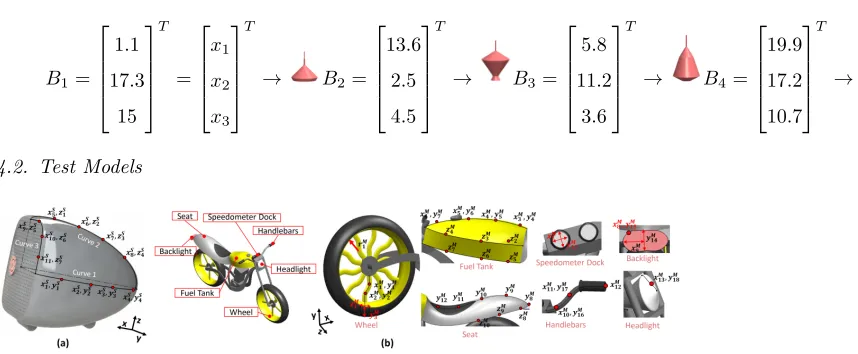
To generate design alternatives with Sf-GDT, first, develop an input CAD
model, shown in Figure 2 (e). This CAD represents a celling lamp and
parame-485
terized with three design parameters,x1,x2andx3. Each design parameter
de-notes the radius of the circular region of the lamp model. Then, form an explicit
design space for this model my defining the parametric ranges as 1≤x1≤20,
1≤x2 ≤20 and 1≤x3 ≤15, and finally, perform following steps to generate
design alternatives for this CAD model:
490
Step 1: Initialize the following parameters:
– Subpopulation size (s) = 2
– Number of designs (N) = 4
– Weight parameter (α) = 5
– Number of design parameters (n) = 3
495
– Ranges of design parameters
Step 2: Randomly generate a population P consists ofN subpopulations. Each
subpopulation contains s = 2 initial designs/solutionsX1g and X2g. The
super script g represents the subpopulation to which these solutions
be-long. The initial population is shown below:
P =h(p1)2×3 (p2)2×3 (p3)2×3 (p4)2×3
(p1)2×3=
X11
X21
=
6.4 9.8 5.0
3.9 16.1 13.6
(p2)2×3=
X12
X22
=
13.6 2.5 5.3
19.1 5.4 10.3
(p3)2×3=
X3 1 X3 2 =
7.4 11.9 3.7
10.9 17.0 12.7
(p4)2×3=
X4 1 X4 2 =
16.6 18.4 5.6
19.8 17.0 10.7
Step 3: Select an initial set of best and worst solutions, one from each
subpopu-lation, using the initial-designs-selection strategy described in Section 3.
This strategy works as follows:
1. Calculate the cost valueU(B) using Equation 7 fors2= 4 combina-500
tions of solutions in populationp1andp2. Then select a combination
which gives lowest (highest) value of the cost as best (worst)
solu-tion. First, calculate the potential energy U1(B) using Equation 2
and number of collapsing designsU2(B) using Equation 4 and then
input these values in Equation 7 to calculateU(B).
505
Calculate cost value forB= [X1 1, X12]:
ScaleX11andX12 between 0 and 1 X11=
6.4
9.8 5.0
T
→
0.28
0.46 0.29
T
X12=
13.6
2.5 5.3
T
→
0.66
0.08 0.31
T
U1(B)=P1p=1
P2
q=p+1 1
L2
pq
= 1
L212
Distance between first and second design ofB=L12=
√
(0.28−0.66)2+(0.46−0.08)2+(0.29−0.31)2=0.54 U1(B)=L12
12
=3.4 U2(B)=1.0
Cost functionU(B)=U1(B)+α×U2(B)=8.4 Similarly, calculate cost for B = [X1
1, X22], B = [X21, X12] and B =
[X1 2, X22]:
B=[X11,X22]→U(B)=9.5
B=[X1
2,X12]→U(B)=0.9 B=[X21,X22]→U(B)=1.0
Solution set [X21, X12] ([X11, X22]) give lowest (highest) cost, therefore,
X1
2 (X11) and X12 (X22) are regarded as the best (worst) solutions of
p1 andp2, respectively.
2. Under the consideration ofX21(X11) andX12(X22) find a best (worst)
solution ofp3. 510
Calculate cost forB= [X1
2, X12, X13]:
X1 2=
3.9
16.1 13.6
T
→
0.15
0.79 0.90
T
X2 1=
13.6
2.5 5.3
T
→
0.66
0.08 0.31
T
X3 1=
7.4
11.9 3.7
T
→
0.34
0.57 0.19
U1(B)=P2p=1
P3
q=p+1 1
L2pq
= 1
L212+
1
L223
L12=
√
(0.15−0.66)2+(0.79−0.08)2+(0.90−0.312=1.06 L23=
√
(0.66−0.34)2+(0.08−0.57)2+(0.31−0.19)2=0.85 U1(B)=L12
12 + 1
L223=2.3 U2(B)=1.0
U(B)=U1(B)+α×U2(B)=7.3 Similarly, calculate cost forB = [X1
2, X12, X23]:
B=[X1
2,X12,X23]→U(B)=24.1
The solution X13 (X23) give lowest (highest) cost value and thus
re-garded as best solution ofp3
3. Select the best (worst) solution of the subpopulationp4
B=[X21,X12,X13,X14]→U(B)=20.7
B=[X1
2,X12,X13,X24]→U(B)=14.2 The best (worst) solution ofp4isX24 (X14).
4. The initial best (worst) solution set isB= [B1, B2, B3, B4] = [X21, X12, X13, X24]
(W = [W1, W2, W3, W4] = [X11, X22, X23, X14]). 515
Step 4: Update solution X11 of p1 based on its best and worst solutions using
Equation 1.
X101=X11+r1(B1− |X11|)−r2(W1− |X11|) =
4.9 12.3 9.6 T Where
r1=
0.6 0.4 0.5 T
r2=
0.02 0.5 0.6 T
Step 5: Calculate the costU(B0) and U(B) forB = [X01
1 , B2, . . . , BN] and B =
[X1
1, B2, . . . , BN], respectively.
B0 = [X101, B2, B3, B4]→U(B0) = 23.7
B= [X11, B2, B3, B4]→U(B) = 64.1
As U(B0) < U(B) so accept the new solution X01
1 and reject the old
Step 6: Similarly, update the solutionX21ofp1.
X201=X21+r1(B1− |X21|)−r2(W1− |X21|) =
3.8 19.6 12.7 T
Step 7: Calculate the cost U(B0) and U(B) using B = [X201, B2, . . . , BN] and
B= [X21, B2, . . . , BN], respectively.
B0 = [X201, B2, B3, B4]→U(B0) = 14.0
B= [X21, B2, B3, B4]→U(B) = 14.2
U(B0)< U(B), so accept the new solutionX201.
Step 8: Obtain the updated subpopulationp0 1
(p01)2×3=
X01
1
X01 2
=
4.9 12.3 9.6
3.8 19.6 12.7
Step 9: Find the new best (B1) and worst (W1) solutions ofp01.
B1=X101=
4.9 12.3 9.6
W1=X201=
3.8 19.6 12.7
Step 10: Replace B1 andW1 withB10 andW10 in the initial set (B = [B10, B2, B3], 520
B= [W10, W2, W3]).
Step 11: Repeat the steps 4 to 10 to obtainp02,p03 andp04.
Step 12: Repeat the steps 4 to 11 until the change in the cost function becomes
negligibly small between a few consecutive iterations. After 13th
itera-tion algorithm converges and the best soluitera-tion of each subpopulaitera-tion is
525
regarded as final optimum design.
B0= [B1, B2, B3, B4]
B1=
1.1 17.3 15 T = x1 x2 x3 T
→ B2=
13.6 2.5 4.5 T
→ B3=
5.8 11.2 3.6 T
→ B4=
19.9 17.2 10.7 T →
[image:25.612.136.565.178.355.2]4.2. Test Models
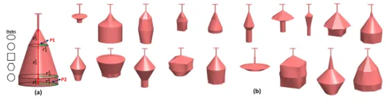
Figure 4: CAD models of (a) speaker and (b) Motorbike with their design parameters.
To validate the performance of Sf-GDT we also utilized more test models,
such as a speaker, a motorbike, a ceiling lamp, and a wine glass, which are shown
530
in Figure 4 (a), (b), Figure 6 (a) and Figure 7 (a), respectively. These models
were selected based on their aesthetic importance. A wine glass defines elegance
of the wine drinker, an aesthetic ceiling lamp and an elegant speaker box and
motorbike design can attract more customers. Except for the motorbike, these
models are single component 3D designs. Where the bike model is composed
535
of several design components. For the complex test model like a motorbike, a
user can first work on the low-level details of the design and then can move to
the high-level details. For example, the user can first explore the form outline
of the design using Sf-GDT and once a collection of different initial base forms
is selected, the designer can then explore further design details by keeping the
540
base form constant. The user may also first explore the design space to create
design alternatives for each component and then assembles these alternative
parts to create the final design. For the motorbike model, only components for
tank, seat, wheels, headlight, backlight, handlebars and speedometer dock. 3D
545
surfaces of the wine glass, ceiling lamp, speaker, fuel tank and seat of motorbike
models are created by interpolating Coons patches between spline curves and
design parameters are defined with these curves. The motorbike’s front and rare
wheels are the 3D solid models.
The speaker model shown in Figure 4 (a) is represented using 22 design
550
parameters (n= 22). The speaker model is created using three spline curves.
First, a quarter section of the speaker model is created using these spline curves.
Then, this section is mirrored first along the y plane and then mirrored along
x-z plane. Curve 1 lies in x-y plane and position of its control points is represented
by the parameter xS1, y1S, xS2, yS2, xS3, yS3, xS4 and y4S and Curve 2 lies in x-z
555
plane and parametersxS5,z1S,xS6, z2S,xS7,z3S,xS8 andz4S denote the position of
its control points. Similarly,xS11,z7S, xS10,z6S, xS9 andz5S represents the control
point position of curve 3. The parameter ranges of the speaker model are given
in Table 1.
Each component of the motorbike model is parameterized separately and
560
consist of total 42 design parameters (n = 42), which are shown in Figure 4
(b). Back wheel is parameterized with 6 continuous design parameter (xM
1 ,
yM
1 ,xM2 ,yM2 ,yM3 andrM1 ) and one discrete parameter (r2M), and front wheel is
created as copy of the back wheel. xM
1 ,xM2 andy1M,yM2 represent the position of
control points in x-axis and y-axis, respectively, andy3M and r1M are the width
565
of the tire and radius of the wheel. The discrete parameter, rM2 , defines the
number of spokes. The fuel tank is created using three spline curves, one in
the y-x plane and two in x-z plane and represented with 14 design parameters.
Similarly, the seat of the motorbike is parameterized with 8 parameters and
created using two spline curves, one in 3D space and other in the x-y plane.
570
The design parametersxM
7 andy13M denotes the width of the speedometer dock
in x-axis and y-axis. The backlight and headlight are represented withxM
8 ,xM9 ,
yM
14, yM15 and xM13, y18M, receptively, where xM9 and y14M adjusts the length and
width of the backlight. The handlebars are also created with spline curves with
design parametersxM10,xM16,xM11,xM17andxM12representing the position of control
points. The parametric ranges of each design parameter are provided in Table
[image:27.612.158.449.186.434.2]1.
Table 1: Parameter ranges for the test models
Speaker Model
5≤xS
1≤150 5≤yS1 ≤90 5≤xS2≤150 5≤yS2 ≤90 5≤xS3≤150
5≤yS
3 ≤90 5≤xS4≤150 5≤yS4 ≤90 5≤xS5≤150 5≤zS1 ≤90
5≤xS
6≤150 5≤z2S≤90 5≤xS7≤150 5≤z3S≤90 5≤xS8≤150
5≤zS
4 ≤90 5.0≤xS9 ≤90 5≤zS5 ≤90 5≤x10S≤90 5≤zS6 ≤90
5≤x11S≤90 5≤z7S≤90
Motorbike Model
6≤rM
1 ≤11 20≤xM1 ≤25 3.5≤yM1 ≤6 20≤xM2 ≤25 3.5≤yM2 ≤5
1.8≤yM
3 ≤2.3 1≤xM3 ≤2 5≤y4M≤7 3≤xM4 ≤8 6≤yM5 ≤12
2≤xM
5 ≤6 6≤yM6 ≤12 10≤xM6 ≤12 6≤yM7 ≤12 4≤zM2 ≤6
4≤zM
3 ≤6 3≤z4M≤5 3.5≤z5M≤5.5 3≤z6M≤6 3.5≤z7M≤5
15≤yM
8 ≤20 17≤y9M≤23 15≤y10M≤20 8≤yM11≤13 10≤y12M≤15
3≤zM
8 ≤7 3≤z9M≤6.5 2≤zM10≤6 2≤xM7 ≤3.5 2≤yM13≤3.5
1.5≤yM
14≤3 2.5≤xM8 ≤4 1≤y15M≤2 4≤xM9 ≤6 2≤xM10≤5
0.8≤yM
16≤3 1≤xM11≤4 2≤yM17≤4 7.5≤xM12≤12 4≤xM13≤7
2≤yM
18≤5 1≤r2M≤7
Celling Lamp Model
1≤yL
1 ≤10 1≤yL2 ≤10 1≤yL3 ≤10 1≤r1L≤20 1≤r2L≤20
Sf-GDT was tested for both constrained and unconstrained design spaces
with different algorithm setting and design space formulation. Design
alterna-tives for the speaker and motorbike models were created with the application
580
of Sf-GDT in the explicitly formalized unconstrained space and can be seen in
Figure 5. A careful inspection of the designs in Figure 5 can reveal that the
gen-erated alternatives by Sf-GDT for each model are distinct from each other to a
great extent. This validates the ability of Sf-GDT to create distinct designs for
any given CAD model. Table 2 provides the algorithm settings and the values
585
of various parameters/criteria such as design alternative (N) and design
param-eters (n) for the test models,U1(B) andU2(B) values, computational time and
Figure 5: Design alternatives generated by Sf-GDT for (a) speaker and (b) motorbike models.
4.2.1. Sf-GDT With Discrete Parameters
A ceiling lamp model (see Figure 6 (a)) is used to demonstrate the
per-590
formance of Sf-GDT for continuous and discrete parameters. The continuous
parameter,yL
1,y2L, andyL3, represents the vertical length of the lamp along the
y-axis, and rL
1 and rL2 are the radii of upper and lower circular region of the
lamp. Where, discrete parameters,rd
1 andrd2, each containing five style forms
(t = 5). These style forms, circle→1, square→2, ellipse→3, hexagon→4 and
595
Table 2: Algorithm setting and the results obtained from Sf-GDT for CAD models utilized
for experimentation.
Designs N n U1(B) U2(B) Maximum value ofU2(B) CT(minutes) i
Figure 5 (a) 20 22 46.43 10 4180 3.72 500
Figure 5 (b) 20 7 151.97 60 1330 1.47 300
Figure 7 (b) 20 10 109.79 0 1900 1.92 300
Figure 7 (c) 20 10 107.94 2 1900 2.10 300
[image:28.612.146.463.581.662.2]octagon→5, are defined on the profile-1 (P1) and the profile-2 (P2) of the lamp
model. Figure 6 (b) shows the design alternatives generated by Sf-GDT based
on both discrete and continuous parameters. The ranges of the continuous
de-sign parameters of ceiling lamp model are given in Table 1. It was observed that
the designs with both continuous and discrete parameters have more variation
600
compared to the designs with only continuous parameters.
Figure 6: (a) Parametric CAD model of ceiling lamp. (b) Design alternatives of ceiling lamp
model generated using Sf-GDT with continuous and discrete parameters.
4.2.2. Sf-GDT in Constrained Design Spaces
Sf-GDT can generate a variety of designs for a given model in the
con-strained and unconcon-strained design spaces. Both the design specifications and
user preferences can be represented by constraints. To validate the performance
605
of Sf-GDT, design specification such as the capacity of a wine glass to store a
certain amount of wine, was given as a geometric constraint. The parametric
representation of the wine glass model is shown in Figure 7 (a). 10 design
pa-rameters (n= 10) are used to represent this model. The design parameteryG
0
is the vertical length of glass stem and the design parameterxG
1, xG2, yG1, xG3, 610
yG
2,xG4,y3G,xG5 andyG4 represent the 2D position of the control points of spline
curve used to create the profile of the glass.
The glass design alternatives in Figure 7 (b) and (c) can store less than or
equal to 200 (≤200) and greater than or equal to 700 (≥700) milliliter (ml)
of wine, respectively. No design in Figure 7 (b) and (c) have violated these
615
[image:29.612.166.446.237.310.2]Figure 7: (a) Parametric representation of a wine glass model. Design alternatives of glass
model generated by Sf-GDT in constrained space with (b) constraint-1 (c) constraint-2. (d)
Design alternatives of glass model generated by utilizing Sf-GDT in an autonomously formed
design space.
4.2.3. Performance of Sf-GDT in Different Design Space Formulations
The performance of Sf-GDT is also validated under different design space
formulation (i.e. explicit, autonomous, and interactive) for the wine glass. The
wine glass designs in Figure 7 (d) are generated by Sf-GDT in an autonomously
620
formed design space with 50% extension of initial design. It can be observed
from Figure 7 (d) that the underlined designs are implausible. These designs
may not be feasible as a final market product. As mentioned before, one way
[image:30.612.149.462.127.216.2]to overcome this issue is to define geometric constraints.
Figure 8: Design alternatives generated for the wine glass model in an interactively formalized
design space.
In interactive space, an initial envelope can be set up either explicitly or
625
autonomously. For example, Figure 8 demonstrate the interactive formulation
of designs. In Figure 8, set-1 contains 17 design alternatives for the wine glass
[image:30.612.151.464.452.543.2]autonomous extension of the initial design. This set contains both plausible and
implausible designs. From this set, one design was selected (checked in red). In
630
the next step, this design was considered as new input model and a new set
(set 2) of designs were created again with 50% autonomous extension of space
around the new design. Note that set 2 contains all the plausible designs. From
this set, two designs were select and new space was formed around the centroid
of these two designs with 30% extension. Afterward, again 30% extension was
635
done for the creation of designs in set-4 and from this final design was selected
and the interactive process was stopped.
4.3. Computational Time (CT)
A PC having an Intel Core i7-5500 CPU, 2.4 GHz processor and 16 GB
memory was used for the experiments in this study, and C++ programming
640
language along with Siemens’ Parasolid APIs were utilized for implementation
and testing of Sf-GDT. We measured the CT taken to obtain results in Figure
5, 6 and 7, which is shown in Table 2; it varied between 1.47 and 21.74 minutes.
The study on the effects of these parameters on CT is important in order to
effectively utilize Sf-GDT. In the proposed approach, CT mainly depends on
645
the number of designs to be generated (N), the dimensionality of the design
space (n) and the size of the subpopulations (s). Increase in the values of these
parameters will increase Sf-GDT’s processing time. As the values of either N
orsincreases CT for Sf-GDT to create designs increases.
4.4. Parameter Tuning
650
For the experiments in this study, α was set equal to 10 except for the
motorbike model for whichα= 20 was utilized because of the high number of
design parameter (n= 42). We recommend the users to set an initial value of
αequal ton/2, which can be altered later depending on the users’ intention to
create complete or semi-non-collapsing designs.
655
It is noteworthy that the value ofU2(B) can be high for the problems with
Instead of dividing the discrete parameter(s) intoN intervals, we divide these
parameters divided intot intervals, where tis the number of style profiles. Ift
is less thanN, then, the number of collapsing designs will increase, which will
660
result in a high value of U2(B). In order to have a low number of collapsing
designs,tshould be greater than or equal toN (t≥N). However, t < N does
not affect the space-filling quality of the designs.
The size of the subpopulations (s) also plays an important role in the
gener-ation of space-filling designs. High values ofscreate diverse initial solutions for
665
Sf-GDT, which facilitates its search for the global optimum solutions. In
con-trast, the application of Sf-GDT with the high values ofscan result in a higher
CT. We recommend settingsto a value higher thann. For the experiments in
the current study,swas set equal to 15 except for the designs in Figure 5 (b).
For thats= 23 was selected.
670
4.5. Convergence of Sf-GDT
The quality of any optimization technique mainly depends on its ability to
provide an optimum solution or a solution close to the global optimum. The
global optimum is a point in search space where the best solution(s) exists.
As the Sf-GDT is based on the optimization technique, therefore, in order to
675
verify the convergence ability to a global optimum its performance is observed
against the number of iterationsi it performs. The convergence ability of
Sf-GDT is analyzed on different test models shown in Figure 5. Sf-Sf-GDT stops the
optimization process when there is no improvement in the cost functionU(B) for
some consecutive iterations (i); at this point, the designs being created reach the
680
optimal position, and the algorithm is considered to converge to its optimality.
Figure 9 shows the plot forU(B) versus ifor the designs in Figure 5, 6 and 7.
A large number of iterations were performed for these models to analyze the
convergence of Sf-GDT. No improvements were observed in U(B) after some
consecutive iterations. For the designs in Figure 6 (b), 7 (b) and 7 (c) there
685
was no improvement occurred after approximately 300th iteration and for the
number of iterations, respectively. The convergence rate of Sf-GDT depends on
the number of designs (N), the dimensionality of the design space (n), and the
total number of geometric constraints.
[image:33.612.173.440.182.312.2]690
Figure 9: Plot showing the cost values versus number of A-GDT iterations for the models in
Figure 5 (a), (b), Figure 6, 7 (b), (c) and (d)
4.6. Comparison with Existing Works
We compared the performance of Sf-GDT with the existing state-of-the-art
techniques in the literature that have been proposed for generative and
space-filling designs. First, we compared the performance of Sf-GDT with Krish’s
GDT [12]. Figure 10 (a) and (b) shows the design points representing designs
695
generated by Krish’s technique for the speaker model in Figure 4 (a) in a 2D
design space. The designs in the 2D space give a better perspective to readers
on how designs generated by [12] are spread in the design space. As mentioned
in section 2, Krish utilized a threshold value, ranging from 0.0 to 1.0, to create
dissimilar designs. The designs in Figure 10 (a) and (b) are created with
thresh-700
old values of 0.5 and 1.0, respectively. It can be seen from the Figure 10 (a) and
(b) that the design points (N = 30) are not uniformly distributed in the design
space especially when the threshold value is 1.0. The designs in Figure 10 (a)
and (b) have space-filling of 7149.9 and 44015, respectively. In case of threshold
equal to 1.0 designs are clustered at the two corners of the design space and
705
also generated by Sf-GDT, which are shown in Figure 10 (c). This gives a
com-parative view to the readers on how Sf-GDT produces design alternatives for
the same CAD model in 2D space. Note that the designs generated by Sf-GDT
had space-filling of 2492.29, which is less than the designs generated by [12].
[image:34.612.151.457.205.282.2]710
Figure 10: Design points created in 2D space by utilizing the technique of [12] with threshold
values of (a) 0.5 and (b) 1.0. (c) Design points created using Sf-GDT. (d) Design alternative
for speaker model created by utilizing the technique of [12].
4.6.1. User Study
Figure 10 (d) shows the designs created by Krish’s technique [12] for the
speaker model in Figure 4 (a) within a 22-dimensional design space, which were
created to visually compare the results of Krish’s technique and Sf-GDT. For
this visual comparison, a user study was conducted to obtain the human
per-715
ception about the quality of designs generated from the two techniques. This
user study included 12 participants to compare the designs in Figure 10 (d) and
5 (a), which are obtained using Krish’s technique and Sf-GDT, respectively. Six
participants had more than two years of design experience in product
devel-opment, and others were selected from the Amazon Mechanical Turk platform.
720
The participants were asked to rate each design in Figure 10 (d) and 5 (a) based
on a Likert scale, with anchors ranging from ”very poor” to ”very good” (1: very
poor, 2: very good, 3: fair, 4: good, 5: very good). The participants involved in
the study had not any information about the techniques used to generate these
designs. This was done to minimize the possibility of a bias decision during
725
design rating. In this study different set of rules was applied to the participants
to ensure the reliability of the obtained results. The designs in Figure 10 (d)
designs. There was a repetition of five designs in each survey. For any
partici-pant, if there was no consistency in the ratings given to the designs and survey
730
was completed in less than five minutes, then that participant’s results were
excluded from the study. Note that the design space utilized for the generation
of alternatives in 10 (d) and 5 (a) was same.
Table 3 summarizes the user study’s results. From the table, it can be
ob-served that the average rating given by the participants to the designs generated
735
with Krish’s technique is lower than those obtained using Sf-GDT. Ten out of
12 participants preferred the designs generated using Sf-GDT, including the
[image:35.612.141.463.333.429.2]experience designers.
Table 3: Results of the user study
Average Grade
User 1 2 3 4 5 6 7 8 9 10 11 12
Sf-GDT 4.55 2.70 3.60 3.25 3.50 3.75 4.00 4.15 4.15 3.10 4.10 3.90
Krish [12] 2.10 3.20 3.65 2.25 3.10 2.45 2.95 4.10 3.75 2.55 2.80 2.75
Space-filling σ µ Skewness p-value
Sf-GDT 46.430 0.630 3.020 0.12
0.00718 Krish [12] 55.039 0.520 3.730 -0.40
A t-test was utilized to statistically examine the results of the user study.
The data obtained from the user study were normally distributed, as the
skew-740
ness value was close to zero and their mean values were approximately equal.
The null hypothesis states that there is no significant difference between the
rat-ings given to the designs generated using Krish’s technique and Sf-GDT. The
p-value obtained from the t-test is less than the significance level of 0.05, this
indicates a stronger evidence against the null hypothesis.
745
From the results of the user study and statistical test, it can also be
con-cluded that Sf-GDT outperforms the Krish’s technique in term of creating


![Figure 10: Design points created in 2D space by utilizing the technique of [12] with thresholdvalues of (a) 0.5 and (b) 1.0](https://thumb-us.123doks.com/thumbv2/123dok_us/1390278.92172/34.612.151.457.205.282/figure-design-points-created-space-utilizing-technique-thresholdvalues.webp)
