Population estimation mining from satellite imagery

Population Estimation Mining From Satellite Imagery

Thesis submitted in accordance with the requirements of the University of Liverpool for the degree of Doctor in Philosophy

by

Kwankamon Dittakan

Abstract

Contents

Abstract i

Contents v

List of Figures viii

Acknowledgement ix

Nomenclature ix

1 Introduction 1

1.1 Introduction . . . 1

1.2 Thesis Objectives . . . 3

1.3 Research Methodology . . . 4

1.4 Contributions . . . 6

1.5 Publications . . . 7

1.6 Thesis Organisation . . . 9

1.7 Summary . . . 9

2 Background and Literature Review 10 2.1 Introduction . . . 10

2.2 Population Estimation using Satellite Image . . . 10

2.3 Image Processing . . . 14

2.3.1 Image Enhancement . . . 15

2.3.2 Image Segmentation . . . 19

2.3.3 Feature Extraction . . . 22

Spatial information . . . 22

Colour . . . 23

Texture . . . 26

2.4 Feature Selection . . . 27

2.5 Data mining and Image Mining . . . 29

2.5.1 Predictive Analysis . . . 31

Regression . . . 33

2.5.2 Frequent Subgraph Mining . . . 34

2.6 Evaluation measure and Statistical Significant evaluation . . . 36

2.7 Summary . . . 38

3 Satellite Image Datasets 39 3.1 Introduction . . . 39

3.2 Test Sites . . . 39

3.3 Satellite Image Collection . . . 43

3.4 Household Image Segmentation . . . 44

3.4.1 Canny Edge detection . . . 45

3.4.2 Hough Transform . . . 47

3.4.3 Least Squares Line Fitting . . . 48

3.4.4 Household Image Segmentation Process . . . 49

3.5 Summary . . . 53

4 Population Estimation Mining using Satellite Imagery: The Graph-Based Ap-proach 54 4.1 Introduction . . . 54

4.2 Quadtree Decomposition . . . 56

4.3 Tree/Graph Representation . . . 58

4.4 Frequent Subgraph Mining and Feature Vector Generation . . . 59

4.5 Feature Selection and Classification . . . 60

4.6 Evaluation . . . 61

4.6.1 Data Representation . . . 61

4.6.2 Feature Selection . . . 65

4.6.3 Number of attributes . . . 67

4.6.4 Classification Generation Method . . . 67

4.7 Discussion . . . 71

4.8 Summary . . . 71

5 Population Estimation Mining using Satellite Imagery: The Colour Histogram Based Approach 73 5.1 Introduction . . . 73

5.2 Colour Histogram Generation . . . 75

5.3 Statistical Colour Metric Calculation . . . 76

5.4 Feature Selection and Classification . . . 77

5.5 Evaluation . . . 77

5.5.3 Number of attributes . . . 83

5.5.4 Classification Generation Method . . . 85

5.6 Discussion . . . 86

5.7 Summary . . . 88

6 Population Estimation Mining using Satellite Imagery: The Texture Based Ap-proach 89 6.1 Introduction . . . 89

6.2 Local Binary Pattern . . . 91

6.3 Statistical Texture Metric Calculation . . . 92

6.4 Feature Selection and Classification . . . 94

6.5 Evaluation . . . 95

6.5.1 Data Representation . . . 95

6.5.2 Feature Selection . . . 99

6.5.3 Number of attributes . . . 100

6.5.4 Classification Generation Method . . . 102

6.6 Discussion . . . 105

6.7 Statistical Comparison of the Proposed Image Classification Approaches . . . . 105

6.8 Summary . . . 110

7 Population Estimation Mining using Satellite Imagery: Regression Analysis 112 7.1 Introduction . . . 112

7.2 Feature Selection and Prediction Model Generation . . . 113

7.3 Evaluation . . . 113

7.4 Discussion . . . 116

7.5 Summary . . . 117

8 A Unified Process for Large Scale Population Estimation Mining Using Satellite Imagery 118 8.1 Introduction . . . 118

8.2 Satellite Image Collection (Step 1) . . . 119

8.3 Segmentation (Step 2) . . . 121

8.4 Duplicated Household Detection and Pruning (Step 3) . . . 125

8.5 Image Representation (Step 4) . . . 125

8.6 Prediction (Step 5) . . . 128

8.7 Evaluation . . . 128

8.7.1 Test Data Collection and Pre-processing . . . 128

8.7.2 Classification based Large Scale Population Estimation Mining . . . . 130

8.7.3 Regression based Large Scale Population Estimation Mining . . . 132

8.9 Summary . . . 135

9 Conclusion 137 9.1 Summary . . . 137

9.2 The Main Findings and Research Contributions . . . 139

9.3 Future Works . . . 142

Bibliography 163 A Additional Algorithms 164 A.1 Introduction . . . 164

A.2 Household Segmentation Algorithm . . . 164

A.3 Graph-Based Image Representation . . . 166

A.4 Colour Histogram Based Representation Algorithm . . . 169

A.5 Texture Based Representation Algorithm . . . 173

A.6 Feature Selection, Classification and Regression Algorithm . . . 173

List of Figures

1.1 Example of a satellite image from the Google Static Map service. . . 5

2.1 Example of satellite images from: (a) an active sensor and (b) a passive sensor. 11 2.2 Example of thresholding for image enhancement . . . 17

2.3 Example of histogram equalisation for image enhancement . . . 18

2.4 Example of the use of an arithmetic operator for image enhancement . . . 18

2.5 Example of threshold based image segmentation . . . 20

2.6 Example of the line based image segmentation . . . 20

2.7 Example of the region based segmentation . . . 21

2.8 Example of quadtree decomposition . . . 23

2.9 The primary colours and secondary colours for the RGB and CMY Colour Spaces. . . 24

2.10 The schematic of RGB and CMY “colour cube” . . . 25

2.11 The relationship between HSV colour space and RGB colour space . . . 26

2.12 Schematic illustrating the feature selection process inspired from [31] . . . 28

2.13 Schematic illustrating KDD meta-process inspired from [69] . . . 29

2.14 Schematic illustrating the generic predictive analysis process . . . 31

2.15 Schematic illustrating the image classification process . . . 32

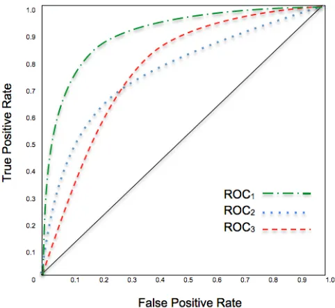
2.16 Example of ROC curves . . . 37

3.1 The location of Horro district, Ethiopia . . . 40

3.2 Ground truth collection at one of the test sites . . . 40

3.3 Site A and Site B locations . . . 41

3.4 The distribution of family size over 120 households . . . 42

3.5 Example of a Site A household . . . 42

3.6 Google Earth image indicating the locations of some of the ground truth house-holds uses . . . 43

3.7 Examples of satellite images for the two different test sites (A and B) . . . 44

3.8 Example of obtained satellite image . . . 45

3.9 Satellite image obtained from test site A. . . 46

3.10 Mapping of one unique line to the Hough parameter space . . . 48

3.12 Household segmentation process for Site A data . . . 51 3.13 Household segmentation process for Site B data . . . 52

4.1 Schematic illustrating the Graph-Based Framework . . . 55 4.2 Schematic illustrating the quadtree decomposition process inspired from [156] . 57 4.3 Example of a quadtree decomposition . . . 58 4.4 The implemented quadtree representation . . . 59 4.5 Bar graph representing the results presented in Table 4.2 . . . 62 4.6 Classification performance in terms of AUC, with respect to the Site A and B

data sets, over a range ofσ values . . . 63 4.7 Nemenyi’s post hoc critical difference diagram (α =0.1) for Objective 1 . . . . 65

4.8 Classification performance in terms of AUC, with respect to the Site A and B data set using the three considered feature selection techniques . . . 66 4.9 Classification performance in terms of AUC with respect to the Site A and B

data sets, over a range of Gain Ratio feature selectionkvalues . . . 68 4.10 Bar graph representing the results of classification performance in term of

AUCs with respect to the Site A and B using different classification genera-tion algorithms . . . 70

5.1 Schematic illustrating the population estimation mining approach using colour histograms . . . 74 5.2 Example of the seven histogram representation for a segmented household image 76 5.3 Bar graph showing classification performance in terms of AUC using different

colour feature space representations (CH,CSandCH+CS) . . . 79 5.4 Nemenyi Significance Diagram for the different colour feature space

represen-tations (α=0.1) . . . 81 5.5 Bar graph showing classification performance in terms of AUCs using different

feature selection methods . . . 82 5.6 Bar graph showing classification performance using different values forkwith

respect to Gain Ratio feature selection . . . 84 5.7 Bar graph showing classification performance using different classification

mod-els . . . 86 5.8 Nemenyi Significance Diagram for the different classification models . . . 87

6.1 Schematic illustrating the population estimation mining approach using LBPs . 90 6.2 The LBP operator . . . 91 6.3 LBP variations . . . 92 6.4 Example of LBP operator . . . 93 6.5 Bar graph showing classification performance in terms of AUC using the seven

6.6 Nemenyi Significance Diagram for the different LBP representations . . . 98

6.7 Bar graph showing classification performance in terms of AUC values using the three different feature selection methods . . . 99

6.8 Line graph showing classification performance using different values forkwith respect to Ch-Squared feature selection . . . 101

6.9 Bar graph showing classification performance using different classification mod-els . . . 103

6.10 Nemenyi Significance Diagram for the different classification models . . . 104

6.11 Bar graph showing classification performance in terms of AUC values using the three different proposed approaches and their variations . . . 108

6.12 Nemenyi Significance Diagram using the three different proposed approaches and their variations . . . 110

7.1 Schematic illustrating the population estimation mining approach using LBPs . 112 7.2 The comparison ofCoe f results with respect to the different regression analysis approaches . . . 115

7.3 The comparison of “approximate” accuracy using Coe f with respect to the different regression analysis approaches . . . 115

8.1 Schematic illustrating the proposed large scale population estimation mining process . . . 119

8.2 An example fragment of a collected “patchwork” of satellite image . . . 121

8.3 Example of the satellite image segmentation process . . . 124

8.4 Example of two duplicate households . . . 126

8.5 The LBP operator . . . 127

Acknowledgement

Chapter 1

Introduction

1.1

Introduction

A census is the procedure of acquiring and collecting information about the nature of the pop-ulation of a given area, it is seen as an important mechanism whereby information can be obtained to support decision makers. Census data is widely used with respect to a variety of central and local government management and planning activities so that informed decisions can be made and budgets set. With respect to the work reported in this thesis census data is equated to population size (in many cases census data incorporates a range of additional data associated with individuals such as occupation, martial status, income bracket and so on). There are many problems associated with the collection of census data, especially in the case of national censuses. The first problem is census budget, the collection of census data requires a considerable resource in terms of money and “manpower”. Another problem is the cost of processing the data after it has been collected. A third issue is that there is often a lack of good will on behalf of a population to participate in a census, even if they are legally required to do so, because people are often suspicious of the motivation behind censuses (especially when collected by government organisations) [45]. These problems are compounded in areas where there are poor communication and transport infrastructures; and/or an extensive, but sparsely populated, hinterland.

case of urban areas (because, as noted above, rural infrastructure tends to be less sophisticated than that of urban areas).

The main advantage of census collection using satellite imagery is reduced cost, the re-quired satellite imagery typically is publicly available from websites such as Google Maps, Google Earth, the US National Aeronautics and Space Administration (NASA) and the US Na-tional Oceanic and Atmospheric Administration (NOAA). The data collection cost is therefore comparatively negligible. This in turn means that census collection can take place whenever data is required and not on some fixed cycle. The second advantage is that it is non-intrusive, thus overcoming the frequently encountered resistance to the collection of census data. In the context of the micro level approach, as presented in this thesis, there is an additional advan-tage that much more detailed census (population) data can be obtained than obtained using the macro level approaches typically reported in the literature. The general disadvantage of the use of remote sensing technology for census data collection is that it is not as accurate as in the case of “on-ground” surveys (there is always a trade of between resource reduction and accuracy); although, as will be demonstrated later in this thesis, good accuracies can be obtained. Another potential disadvantage is that it is desirable, for best results, that up to date satellite imagery is used. Typically Google Earth and the Google static map service update their imagery over a one to three years cycle depending on the region. In case of the Ethiopia data used for evalu-ation purpose later in this thesis a three year cycle was noted, probably because of the remote nature of the region and because rural areas feature less annual change than urban areas.

The fundamental idea presented in this thesis is thus that census (population size) data can be collected using classification and/or regression techniques applied to relevant satellite imagery. The research described is thus directed at mechanisms for the end-to-end process of building a classification or regression model that can predict household “family size” according to the nature of households captured from satellite imagery. More specifically the idea is to segment satellite images so as to obtain pixel collections describing individual households and represent these collections using some appropriate representation to which a classifier or regression model generator can be applied.

associated research issues and challenges are presented in Section 1.2. The research methodol-ogy used to address the research challenges, including the “criteria for success”, is presented in Section 1.3. The contributions of the research work, including an itemisation of the published work to date arising from the research, is presented in Section 1.4. A summary of the publica-tions [36, 37, 38, 39, 197] that have arisen out of the work presented in this thesis is given in Section 1.5. Followed by an overview of the rest of this thesis in Section 1.6 and a summary of this chapter in Section 1.7.

1.2

Thesis Objectives

From the foregoing the research domain at which this thesis is directed is thus concerned with the investigation, realisation and evaluation of algorithms and processes that can be used to build classification/regression models for the purpose of collecting population census data. This research objective is encapsulated by the following research question:

What are the most appropriate end-to-end computational processes required to collect

population census data from satellite imagery using classification and regression techniques?

The resolution of this research question encompass a number of research challenges. These are articulated below in the form of a series of subsidiary research questions:

1. What are the most appropriate mechanisms for segmenting a given satellite image so that appropriate individual household sub-images (if any) can be identified?

2. Given a set of identified household images how should the content of those images be represented so that compatibility with classification and regression model generation is achieved while at the same time ensuring that key information is retained?

3. When representing household images what is the nature of the key information to be captured?

4. What are the most appropriate classification/regression techniques for predicting census data given a processed collection of household images?

5. What is the process for conducting a large scale census comprising many satellite im-ages?

6. In the context of conducting large scale surveys how can issues associated with “over-lapping” satellite images best be resolved?

1.3

Research Methodology

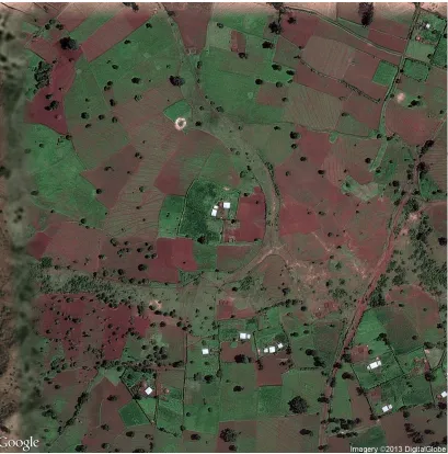
To act as a focus for the work two rural areas of the Ethiopian hinterland, located some 300 km to the northwest of Addis Ababa, were used. These areas were selected because details concerning individual households had been collected by University of Liverpool field staff. This information included household size in terms of number of people normally resident and location latitude and longitude. Figure 1.1 shows part of a satellite image covering one of these districts. From the figure we can clearly observe several households. The data was collected as part of a field study, investigating the health of chickens, conducted by the School of Veteri-nary Science at the University of Liverpool in May 2011 and July 2012. The data was collected using a sampling process; thus, given a particular village data for only some of the households, dispersed across the village, was available. For the purpose of the research, satellite images were obtained using the Google Earth and Google Static Map services (although clearly other forms of satellite imagery could equally well have been used). The collected latitude and lon-gitude data was used to identify appropriate satellite images that covered the geographical area of interest.

The first step in the adopted methodology was to investigate mechanisms whereby the households could be isolated using image segmentation techniques. This included mechanisms that could be adopted for image cleaning. The idea was to produce a set of “household im-ages” that would provide the foundation for further processing. So that appropriate classifica-tion/regression models could be generated. The second step was to investigate methods for rep-resenting household images in such a way that: (i) compatibility with classification/regression model generation techniques was obtained and (ii) information loss was minimised. A review of the existing literature concerning image classification suggested three broad categories of representation technique; (i) graph-based, (ii) colour histogram based and (iii) texture based.

of the data presented in the tables, and the second (where theH0 hypothesis has been rejected) is to attempt to identify where the statistical differences occur. In the context of the regression models the measures used were: correlation coefficient, Mean Absolute Error (MAE) and Root Mean Squared Error (RMSE).

The next and final stage of the adopted methodology was to consider the process for con-ducting large scale population estimation mining using the techniques considered. To illustrate the process an entire village and its surrounding lands were considered, as opposed to individ-ual households. For this purpose a rural area of Ethiopian, measuring 42.7km2, was selected that had a known (or at least reported) population size. Prior to conducting the large scale popu-lation estimation mining process it was necessary to first investigate mechanisms for acquiring large sets of satellite images (a “patchwork” of 600 satellite images was used for the study). This was followed by an investigation of the mechanisms for identifying individual households in such a way that the “overlap problem” could be addressed (the issue of the same household appearing in two or more overlapping satellite images). Evaluation was again conducted by comparing the reported (known) population size with the predicted population size using the same metrics as used previously (see above).

1.4

Contributions

The contributions of the research work presented in this thesis can be summarised as follows:

1. A novel approach for image segmentation specifically designed for segmenting individ-ual households featured in a satellite image data set.

2. A household image representation founded on a quadtree based hierarchical decompo-sition of space together with a frequent subgraph mining algorithm for dimensionality reduction. The identified frequent subgraphs were arranged into a feature vector for-mat, one vector per household, suited for input into a classification or regression model generation algorithm.

3. A household image representation founded on a colour histogram based approach. More specifically an image representation founded on multiple histograms extracted from var-ious colour channels; a feature vector format was again used.

4. A household image representation founded on the concept of “texture” analysis. More specifically usage of Local Binary Patterns (LBPs), as before a feature vector format was again derived.

5. A detailed comparison of the proposed household image representations.

7. An analysis of a number of regression model generation algorithms so as to identify the most appropriate in the context of population estimation prediction from satellite data.

8. An effective mechanism for satellite image collection using the Google Static Maps ser-vice to obtain satellite image data for a specified area.

9. A novel approach for household detection specifically designed for the purpose of iden-tifying and segmenting individual households featured in a satellite image data set cov-ering a prescribed area.

10. A mechanism for detecting duplicated households in a given satellite image data collec-tion so as to address the image “overlap” problem.

11. An end-to-end process for conducting large scale population estimation mining using satellite data.

12. Overall, the thesis presents an approach of population estimation founded on known techniques, but combining a new and novel methodology.

1.5

Publications

A number of research publications have arisen out of the work presented in this thesis. These are itemised below, in each case a short summary is given and a reference to where the material features in this thesis.

Kwankamon Dittakan, Frans Coenen, Rob Christley:Towards The Collection of Census Data From Satellite Imagery Using Data Mining: A Study With Respect to the Ethiopian

Hin-terland. SGAI Conf. 2012: 405-418.

This paper was the first to describe the proposed framework for remotely collecting cen-sus data using satellite imagery and data mining (classification). The main idea presented in this paper was that classifiers can be built that classify household satellite images to produce census data, provided an appropriate representation is used. The proposed repre-sentation was founded on the idea of representing segmented households using a colour histogram based formalism. The presented evaluation indicated that accurate census data can be collected using the proposed approach at a significantly reduced overall cost com-pared to traditional approaches to collecting such data. The work summarises some of the material presented in Chapter 5 where the detail of the proposed colour histogram based representation is presented.

Kwankamon Dittakan, Frans Coenen, Rob Christley:Satellite Image Mining for Census

Col-lection: A Comparative Study with Respect to the Ethiopian Hinterland. MLDM 2013:

As in the case of the previous paper this paper also presented the idea of using satellite imagery to generate census data from satellite imagery using a classifier for household size census prediction. The paper processes the Local Binary Pattern (LBP) representa-tion. The presented evaluation indicated a particular variation of the LBP representation, calledLBP8,1, tended to produce the best results. The work summarises some of the

ma-terial presented in Chapter 6 where the fundamental idea of texture analysis for satellite image representation, more specifically the LBP representation, is described.

Kwankamon Dittakan, Frans Coenen, Rob Christley, Maya Wardeh: Population Estimation

Mining Using Satellite Imagery. DaWaK 2013: 285-296.

As in the case of the previous two papers, this paper also described the framework for population estimation mining (census mining) founded on the concept of applying clas-sification techniques to satellite imagery. However, the particular note was the subgraph feature vector representation that was used to encode household imagery. The proposed framework was evaluated using test data, collected from two villages in the Ethiopian hinterland, also used in this thesis. The conducted evaluation indicated that when using a minimum support threshold ofσ =10 for the subgraph mining, good results could be obtained. The work summarises some of the material presented in Chapter 4 where the detail of the graph-based representation, using quadtree decomposition together with frequent subgraph mining, is described.

Kwankamon Dittakan, Frans Coenen, Rob Christley, Maya Wardeh:A Comparative Study of Three Image Representations for Population Estimation Mining Using Remote Sensing

Imagery. ADMA 2013: 253-264.

This paper presents a summary of the usage of the three representation presented in this thesis for population estimation mining: (i) colour histogram based, (ii) Local Binary Pattern (LBP) based and (iii) graph-based. The presented evaluation indicated that the

LBP8,1variation of the texture based representation produced the best overall result. The

work summarises some of the material presented in Chapter 6, especially Sub-section 6.7.

Wen Yu, Frans Coenen, Michele Zito, Kwankamon Dittakan: Classification of 3D Surface

Data Using the Concept of Vertex Unique Labelled Subgraphs. ICDM Workshops 2014:

47-54.

1.6

Thesis Organisation

The organisation of the rest of this thesis is as follows. Chapter 2 provides an extensive litera-ture review of population estimation using satellite imagery and the previous work concerning the technologies that feature in this thesis, including discussion concerning the processing of 2D image data. Chapter 3 describes the nature of the satellite image data sets, and the applica-tion domain, used as a focus for the work presented in this thesis. The nature of the necessary data preparation and image preprocessing applied to these data sets is also presented in this chapter. The three considered feature extraction approaches used for satellite image repre-sentation are described in the following three chapters. Chapter 4 presents the graph-based approach founded on a quadtree storage mechanism and a hierarchical decomposition coupled with the application of frequent subgraph mining techniques to identify frequently occurring “patterns” hidden in the identified household image data. Chapter 5 considers the proposed colour analysis based approach whereby colour histograms are used together with colour sta-tistical features representing the identified household images. Chapter 6 presents the proposed texture analysis based approach which uses LBPs and texture statistical features to extract and represent the texture properties from identified household images. The evaluation of the three representations is also presented in Chapter 6. Chapter 7 is an investigation of the use of regres-sion analysis for population size estimation. Chapter 8 then describes the proposed end-to-end large scale population estimation mining process and the evaluation of this process using a large scale study. Finally, in Chapter 9, the thesis is concluded with a summary, presentation and discussion of the main findings in the context of the research question and sub-questions identified above and some suggestions for future work.

1.7

Summary

Chapter 2

Background and Literature Review

2.1

Introduction

A review of the background and previous work with respect to the research presented in this thesis is presented in this chapter. The chapter starts, Section 2.2, with a review of the “popula-tion estima“popula-tion using satellite imagery” applica“popula-tion domain. The work described in this thesis is concerned with the application of data mining techniques, more specifically image mining tech-niques, for the purpose of population estimation using satellite image data. The main challenge in this context is how best to extract and represent image features so that mining algorithms can be applied. Image feature extraction and representation, and especially satellite image feature extraction and representation, is a central theme of this thesis. Image pre-processing is therefore discussed in Section 2.3 with a particular focus on: image enhancement, image segmentation and feature extraction. In addition, prior to the application of any data mining process, it is typically necessary, both from a computational efficiency and a computational effectiveness perspective, to reduce the dimensionality of the feature space by applying some form of feature selection. This is discussed further in Section 2.4. The chapter is then continued with Section 2.5 where some background concerning the domain of data mining is presented and more detail concerning the associated sub-domains of image mining and prediction. With respect to the latter both classification and regression are considered. A discussion concerning frequent subgraph mining is also presented because one of the representations presented uses the idea of extracting features from satellite images using graph/tree based techniques, which are then converted into a feature vector format using frequent subgraph mining. The mecha-nism adopted later in this thesis for the statistical comparison of different prediction models is presented in Section 2.6. Finally a chapter summary is presented in Section 2.7.

2.2

Population Estimation using Satellite Image

an image. Examples of omitted energy sources include: (i) sunlight, (ii) wavelengths outside of the range of human vision, (iii) the “upwelling energy” which is radiated from the earth, and (iv) artificial sources [149]. The sensors, that may be mounted on aircraft or spacecraft, are classified into two categories: (i) passive and (ii) active. The distinction is that there is no energy source of radiation provided in the case of passive sensors such as cameras, multi-spectral scanners, thermal scanners and microwave radiometers. An example image obtained from a passive sensor is given in Figure 2.1(a). In contrast active sensors provided a built-in source of radiation, examples built-include Radio Detection and Rangbuilt-ing (RADAR) and Light Detection and Ranging (LIDAR) [91]. Figure 2.1(b) presents an example of a satellite image obtained using LIDAR technology. Satellite imagery provides an effective means of observing and quantifying the complexities of the surface of the earth.

Figure 2.1: Example of satellite images from: (a) an active sensor and (b) a passive sensor.

Example applications where satellite images have been used include: (i) agriculture, (ii) forestry, (iii) land usage/land coverage studies, (iv) disaster management, (v) defence and se-curity, (vi) natural resource management, (vii) climate monitoring and (viii) marine and coastal zone monitoring [6, 19, 82, 131, 162, 171, 184].

(ii) census data collection and (iii) processing of the results. Traditionally there are two main approaches to census collection [134]:

1. Mailing of questionnaires to a list of household addresses, either by post or by electronic means, and asking individual householders to takes responsibility for completing and returning questionnaires.

2. Using ground staff to visit individual households in order to interview householders and obtain the desired census information.

As noted in Chapter 1, traditional population census collection (using either of the above) requires significant resource (money, staff and time) for both data collection and post-processing. In the context of the cost of census collection the UK Office for National Statistics (UKONS) reported that the UK 2011 census cost approximately £480 million; a figure that included both the cost of data collection and the cost of post processing. This is a considerable outgoing although UKONS notes that this cost “breaks down to less than £1 per person per year over the 12-year planning and operational cycle of the census” [48, 120, 133, 152]. The US 2010 census is reported to have cost $13 billion, approximately $42 per capita; by comparison, the 2010 census per-capita cost for China was about $1 and for India was $0.4 [125]. In December 2010 the US Government Accountability Office (GAO) noted that the cost of conducting US censuses had approximately doubled each decade since 1970 [164]. According to the Aus-tralian Bureau of Statistics the AusAus-tralian 2011 census cost around AUD 440 million, about AUD 19 per person; whilst the 2006 census cost around AUD 300 million. Census collection is thus expensive and is becoming more so. Furthermore the resource required with respect to rural areas is typically greater to that required in urban areas because the communication and transport infrastructure in rural areas tends to be less well developed. Of course the cost has to be offset against the benefits that census data provides. UKONS argues that the cost “has to be set against its value in helping central and local government to allocate annually many billions of pounds of funding to communities” [58, 142].

Other than the cost associated with traditional census collection methods there are a number of additional disadvantages:

1. Where the intention is to collect census data using electronic means, for a variety of reasons, many people remain unconnected to the internet. In the context of the UK 2011 census UKONS reported that the most frequently cited reason for households not to have internet access was because of a “life style” decision not to. In less affluent parts of the world internet accessibility and usage is much lower (although arguably set to increase).

A solution to the above disadvantages, and that advocated in this thesis, is to use satellite imagery for the purpose of population estimation. Population estimation has been a subject of researched amongst the Geographic Information Systems (GIS) and remote sensing commu-nities for some time. From the literature we can broadly divide this research activity into two categories: (i) areal interpolation and (ii) statistical modelling [189]. In the areal interpolation category existing census information concerning some geographic area is used as an input to an interpolation algorithm to obtain a population estimation for a wider or alternative geographic area [99]. Statistical modelling in turn is concerned with the relationship between population size or density and data obtained from GIS and/or satellite imagery. The work presented in this thesis can be said to fall into the second category. The existing work on statistical modelling for the purpose of population estimation can be further categorised according to the nature of the data on which the population estimation generation is based, namely: (i) light intensity, (ii) land usage, (iii) dwelling unit count, (iv) image pixel characteristics and (v) physical or socio-economic characteristics.

The central idea on which the first category is based is that there is a functional relationship between population size and the amount of night time light emanating from an area. In [3], [26], [119] and [144] the relationship between population density and light frequency was analysed in order to convert light frequency into a population density metric using a luminous saturation measure obtained from the Defence Meteorological Satellite Program (DMSP) Operational Linesman System (OSL). In [144] the reported evaluation was directed at Japan and China, whereas in [26] and [119] it was directed at China only. In [3] the evaluation was directed at a population estimation of the Brazilian Amazon.

Work within the second category is directed at the correlation between population density and different types of land usage. The idea is to determine population densities according to land usage with respect to a set of one or more sample areas and apply this knowledge to additional areas. Land usage categories are typically identified from satellite image data. In [96] it is suggested that population densities for different types of land usage can be determined from sample surveys or census statistics. Four different types of land usage were extracted from four different cities in California, USA, and population densities computed. In [116], six types of land usage were identified in the context of Landsat TM satellite images centred on Atlanta, USA. A regression model was then applied to produce population densities for Atlanta.

“fea-ture extraction techniques” have been developed for this purpose [74]. In [2] a dwelling unit count based approach is presented using IKONOS satellite images of the Al Shaabia district in Khartoum, Sudan. The dwelling unit count approach has some similarity with respect to the work represented in this thesis.

In the fourth category, the relationship between image pixel characteristics and population densities are examined. The image pixel characteristics can be represented using a variety of mechanisms, but common examples include: mechanisms based on the spectral reflectance value of image pixels and image texture analysis mechanisms. Examples of using pixel char-acteristics for population estimation are presented in [87] and [103]. In [87] a system was pre-sented whereby texture analysis was applied to Google Earth satellite images, using block sizes of 64x64 and 32x32 pixels, to estimate population densities with respect to cities in Pakistan. In [103] a variety of features were used, including: spectra signatures, principle components, vegetation indices, fraction images, texture and temperature. These features were extracted from Landsat ETM+ satellite images and used to measure population density in the city of Indianapolis, Indiana, USA.

The final category of population estimation is founded on the usage of various kinds of physical and socioeconomic information which is then interpolated to give population estima-tions. For example, information about demography, topography and transportation networks have all been used to estimate population size. In [114] a mechanism was presented for esti-mating population size by determining the correlation between the population in urban areas and the distance to the nearest Central Business Distract (CBD), distance to major roads, slope and the age of the community.

What all the above approaches to population estimation modelling have in common is that they are focussed on regions or areas rather than specific households as in the case of the work presented in this thesis. As far as the author is aware the approach presented in this thesis is entirely unique.

2.3

Image Processing

As noted above, before image mining of any form can be conducted the image set of inter-est must be pre-processed in an appropriate manner. In the context of the work presented in this thesis three image pre-processing operations are used: (i) image enhancement, (ii) image segmentation and (iii) feature extraction.

Image segmentation is the process of grouping image pixels that share some form of com-monality. The groupings are usually referred to asregionsorobjects. The typical goal is to facilitate image analysis. Image segmentation is usually achieved by identifying objects and boundaries. In the case of the work presented in this thesis image segmentation was applied in order to isolate individual households, an overview of the adopted image segmentation process is given in Sub-section 2.3.2.

Feature extraction is the process of representing images, or image segments, according to image content. There are various content features that may be used for this purpose such as colour, texture and spatial layout [28]. Colour features are the simplest to obtained as they can be extracted directly in terms of pixel intensities. Texture is normally considered in terms of some form of prescribed spatial pattern template describing the relative position of colour, texture or shape information [179]. A review of existing work directed at feature extraction (and representation), in the context of the work presented in this thesis, is thus given in Sub-section 2.3.3.

2.3.1 Image Enhancement

A review of image enhancement processes, in the context of this thesis, is presented in this sub-section. As noted above, the objective of image enhancement is to improve the quality of an image so as to improve the effectiveness of any further processing to be applied. Typi-cally image enhancement includes: (i) “sharpening” (de-blurring), (ii) contrast improvement, (iii) brightens adjustment and (iv) noise removal. Image enhancement has been shown to be advantageous with respect to many image analysis applications such as: medical image analy-sis [161], biometric authentication (such as face detection and fingerprint detection) [90, 153] and satellite image analysis [84]. The latter is of particular relevance with respect to the work presented in this thesis.

Image enhancement can be generally described as the process of transforming an input image comprised of an ordered collection of pixelsR, using a functiont, into an output image comprised of an ordered collection of pixelsS(Equation 2.1).

S=t(R) (2.1)

The challenge of image enhancement is quantifying the criterion for the enhancement; a large number of image enhancement techniques are empirical and require interactive procedures to obtain satisfactory results.

1. Thresholding, which was applied to each layer of the Hue-Saturation-Value (HSV) satellite image colour space so that the households of interest were more clearly defined and so that features such as rivers and roads were eliminated from images.

2. Arithmetic and logic operations, which were used to combine an input image with an another image (possibly a mask) so as to produce a single enhanced image.

3. Histogram Equalisation, which was used adjust the image contrast so that it was con-sistent across a given collection of satellite images.

Each of the above is described in further detail in the remainder of this sub-section.

Thresholding is an image enhancement process used to separate image objects of interest (the “foreground”) from the rest of an image (the “background”) by converting a given image into a binary, black and white, image where white regions represent the foreground and black regions the background. The method assumes that the colour features associated with the foreground is somehow distinct from the colour features associated with the background. More formally we can define thresholding using the following:

s=

(

1 r>threshold

0 r≤threshold (2.2)

wheres∈Sandr∈R.

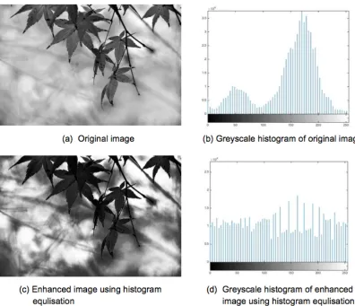
Thresholding methods can be divided into two main categories: (i) global and (ii) local [146]. Global thresholding methods use a threshold value applicable to an entire image; the threshold value is often based on an estimation of the boundary between foreground and back-ground as displayed in an intensity histogram (hence it is often referred to as a “point pro-cessing” operation). Local methods use an adaptive threshold whereby different threshold values are derived from local area information [72]. Figure 2.2 gives an example of threshold-ing. Figure 2.2(a) gives the original image while Figure 2.2(b) gives the enhanced image after thresholding has been applied.

Figure 2.2: Example of thresholding for image enhancement

after histogram equalisation has been applied and its associated greyscale histogram in Fig-ure 2.3(d). From the figFig-ure it can be observed that the histogram is more “dispersed” after histogram equalisation.

Arithmetic and logic operations are often used for the purpose of image enhancement by combining an input image with one or more other images so as to produce an enhanced im-age. Such operations are performed on a pixel-by-pixel basics, as in the case of thresholding. Typical arithmetic operations that may be applied are addition and subtraction; typical logic operations areAND,ORandNOT [55].

As the name suggests, using the addition operator the corresponding pixel values for two equal sized input images are each summed to produce a new image of the same size as the first two. A common variant of the addition operator is to simply add a constant value to each pixel in a single input image [124]. In the case of the subtraction operator the pixel values are subtracted from one another; alternatively a constant may be subtracted with respect to the pixels in a single input image [85].

The logical operators are used, in a similar manner to the arithmetic operations, on a pixel-by-pixel basics; they are typically used for the operation to binary valued or greyscale images. The operation of theAND, ORandNOT operators is as standard. To give one example the logical NOT operator is used to invert pixel values, so that dark areas in the input image become light areas in the output image and vice versa [33, 56].

Figure 2.4 gives an example of arithmetic/logic enhancement. Figure 2.4 (a) gives the original image and Figure 2.4(b) an enhanced image obtained by adding the constant value of 100 to the original image.

Figure 2.3: Example of histogram equalisation for image enhancement

2.3.2 Image Segmentation

An overview of image segmentation is presented in this sub-section. In the context of the work presented in this thesis segmentation was used to isolate individual households. More generally image segmentation is used in situations where some part of an image, or some region within an object, is required in the context of further image analysis [137]. In [55] image segmentation is defined as the process of partitioning a digital image into semantically interpretable regions that are more meaningful and easier to analyse with respect to a particular application then if the entire image was taken into consideration. Segmentation has been usefully employed with respect to a variety of applications [32] such as: (i) medical applications (isolating tumours and other pathologies, measuring tissue volumes, computer guided surgery, diagnosis, treatment planning and the study of anatomical structure) [46, 112, 127], (ii) geoscience (location of objects such as roads, forests and crops in satellite images) [11, 54], (iii) face recognition [13] and (iv) finger print recognition [181].

Segmentation is typically conducted according to some characteristic image feature such as colour, line, intensity or texture. There are various image segmentation methods that have been proposed. A well documented categorisation of image segmentation methods is: (i) threshold based segmentation, (ii) edge based segmentation and (iii) region based segmentation. Each is discussed in further detail below.

Threshold based segmentation is the simplest segmentation method. Note that this tech-nique may be applied for both enhancement (see Sub-section 2.3.1) and segmentation. With respect to segmentation, thresholding is used to transform a greyscale image into a binary im-age. The idea of threshold based segmentation is to replace each pixel in an image with a black pixel if the image intensity of the pixelIi,jis less than the threshold valueT(that is,Ii,j<T), or

a white pixel if the image intensity is greater than that constant [192, 193]. Figure 2.5 presents an example of threshold based segmentation; Figure 2.5(a) is the original image while Figure 2.5(b) is the processed image.

In edge based segmentation the edges in an image are identified. Ideally the detected edges from the given image represent object boundaries and can thus be used to define these objects. Image segmentation using edges is typically a three step processes: (i) compute an edge image containing all edges of an original image, (ii) process the edge images so that only closed object boundaries remain, and (iii) transform the result to an ordinary segmented image by filling in the object boundaries [17, 81]. An example of edge based segmentation is shown in Figure 2.6; Figure 2.6(a) is the original image, while Figure 2.6(b) is the processed image using edge based segmentation.

Figure 2.5: Example of threshold based image segmentation

of the image where each pixel is in its own segment, (ii) merge those adjacent segment pairs that are most similar, and (iii) repeat step (ii) until no more segments can be merged remain. The central element of the merging approach is the similarity criterion used to decide whether two segments should be merged or not. This criterion may be based on grey value similarity (such as the difference in average grey value, or the maximum or minimum grey value differ-ence between segments), the edge strength of the boundary between the segments, the texture of the segments, or one of many other possibilities. The basic approach to image segmentation using splitting is as follows: (i) obtain an initial segmentation of the image where the entire image is in a single segment, (ii) where possible split each segment into two “homogeneous” sub-segments, and (iii) repeat step (ii) until no more splitting can take place. The criterion for the homogeneity of a segment may be the variance of its grey values, the variance of its texture, the occurrence of strong internal edges, or various other criteria. Figure 2.7 presents an example of region based image segmentation; Figure 2.7(a) is the original image, and Figure 2.7(b) is the processed image using region based segmentation.

Figure 2.7: Example of the region based segmentation

The merging and the splitting approaches may be combined: the basic splitting approach is often enhanced by combining it with a merging approach, where inhomogeneous segments are split into simple geometric forms recursively. This of course creates arbitrary segment boundaries, and merge steps are included into the process to remove incorrect boundaries.

defined by some kind of boundary, therefore line or edge segmentation is appropriated.

2.3.3 Feature Extraction

An overview of image feature extraction mechanisms is presented in this sub-section. A neces-sary precursor for the application of image mining is that the key properties or characteristics of the image set to be mined need to be extracted and represented so as to facilitate the desired im-age mining [176]. It is not possible to mine imim-ages directly because of the prohibitive amount of pixel data that would have to be considered. The most commonly used representation used with respect to prediction (classification and regression) is the feature vector representation. Feature extraction and representation is central to the research presented in this thesis, three alternatives are considered: (i) graph-based, (ii) colour histogram based and (iii) texture based, all three result in a feature vector representation. Given the significance of feature extraction with respect to this thesis a review of previous work in this area is therefore presented in this section.

In the early work on feature extraction from images the process was not based on image content but on the textual annotation of images, see for example [21, 173]. However, the automatic generation of textual annotations for images is not a realistic one, the text-based approaches require manual annotation which is both resource intensive and challenging [117]. More recently techniques based on visual information extraction have been developed, thus content-based feature extraction instead of text based feature extraction; see for example [24, 93, 143]. In content based feature extraction the features considered are quantifiable properties of an image. These properties/features can be divided into two categories: (i) general features and (ii) domain-specific features. General features are application independent and include features such as colour, texture and spatial layout. The nature of such general features can be further divided into: (i) pixel-level features such as colour and pixel location (the colour histogram based technique for population mining from satellite images presented later in this thesis falls into this category), (ii) local features calculated over a sub-area or region of an image, and (iii) global features calculated over an entire image such as texture based feature extraction techniques (the graph and LBP based approach presented later in this thesis fall into this category). Domain-specific features are application dependent features, for example elements of the human face as used in face recognition [28]. With respect to the work presented in this thesis the general feature extraction methods used are focussed on three basic types of features: (i) spatial information, (ii) colour and (iii) texture. Each is thus briefly considered in some further detail below.

Spatial information

histograms, however the spatial locations within the image will be different. Spatial infor-mation is often represented using a graph representation [51, 157]. Examples of graph-based structural image feature representations include: Attributed Graphs (AGs), Function Describe Graphs (FDGs) and Quadtrees. 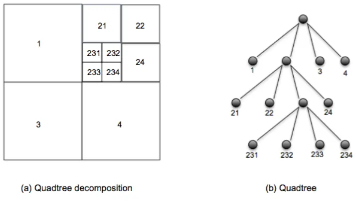The advantages of graph-based representations are their general applicability [29] and their invariance to rotation and translation [92].

One of the most common methods for spatial information feature extraction is quadtree decomposition. In a quadtree every node in the tree, apart from the leaf nodes, has four “chil-dren” labelled North-West (NW), North-East (NE), South-West (SW), and South-East (SE). The image is partitioned into four quadrants at each hierarchical level, however it is usually un-necessary to decompose all branches down to the same level. If a parent node has four children of the same value (node label) the decomposition can be stopped at the parent node. Figure 2.8 gives an example of a quadtree decomposition, Figure 2.8(a) illustrates the decomposition while Figure 2.8(b) presents the resulting tree [170].

Figure 2.8: Example of quadtree decomposition

Note that in Figure 2.8, the coding reflects the decomposition (1=NW, 2=NE, 3=SW and 4= SE). Quadtrees have been applied widely with respect to image analysis including satellite image analysis; examples where quadtree decomposition has been used in the context of satellite imagery can be found in [195] and [128]. Quadtree decomposition was also used in the context of the work presented in this thesis; this will be discussed further in Chapter 4.

Colour

implemen-tation, (ii) effectiveness with respect to many applications, (iii) invariance to image rotation and (iv) low storage requirement [28]. In general, colour is represented using the concept of

a colour space (also known as colour mode, model or system). There are various existing

colour spaces: (i) RGB (Red, Green, and Blue), (ii) CMYK (Cyan, Magenta, Yellow, and Key (black)), (iii) HSV (Hue, Saturation, and Value) and (iv) greyscale.

Figure 2.9: The primary colours and secondary colours for the RGB and CMY Colour Spaces.

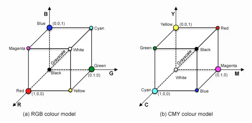
The RGB colour space is most commonly used for images, particularly for the representa-tion and display of images in electronic systems, such as cameras and computers. RGB is what is termed an “additive” colour space, which means that individual pixel colours are created by combing a number of light channels (see Figure 2.9(a)). In the case of the RGB colour space the channels are: Red (R), Green (G) and Blue (B); hence RGB. The wavelengths of the red, green and blue channels were adopted solely for the purpose of standardisation and not to achieve equivalence with visible colours [80]. The RGB colour space can be represented in terms of a 3D coordination system where the originh0,0,0i is black andh1,1,1i is white. All values for red, green and blue are assumed to be in the range of 256 intensity values. Figure 2.10(a) shows the RGB colour space with the primary colours red, green and blue and the secondary colours yellows, cyan and magenta. The secondary colours are produced from the combination of two primary colours. Greyscale comprises the values along the dashed line connecting black to white.

Figure 2.10: The schematic of RGB and CMY “colour cube”

but in practice combining these three colours for printing purposes does not produce pure black. To generate pure black (the predominant colour in printing), black (K) is given as a fourth colour stream leading to the CMYK colour space.

The CMY colour space can be represented by a 3D coordinate system in the same way as the RGB colour space. Againh0,0,0iis black andh1,1,1iis white. Figure 2.10(b) shows the CMY colour space with the primary colours cyan, magenta and yellow and the secondary colours red, green and blue. As in the case of the RGB colour space the secondary colours are produced from the combination of two primary colours. As before greyscale comprises the values along the dashed line connecting black to white.

Figure 2.11: The relationship between HSV colour space and RGB colour space

Greyscale colour refers to a range of shades of grey from black to white. The intermediate shades of grey are represented by equal values for the three primary or pigments colours when using the RGB or CMY colour spaces. Because only 8 bits are required for greyscale (as opposed to 24 for RGB or CMY) the colour space is sometimes called 8-bit greyscale [158, 196].

Three of the above colour spaces (RGB, HSV and greyscale) were used with respect to pre-processing of the raw satellite image data considered in this thesis.

Texture

Feature extraction in terms of texture refers to processes whereby individual pixels are defined in terms of their neighbours. Image texture has been widely used with respect to various ap-plications, for example content-based image retrieval, image classification, pattern recognition and computer vision [27, 52, 88]; image classification is of course of particular interest with respect to the work presented in this thesis. In more detail texture is described in terms of texture primitives or texture elements (texels), based in turn on “tone and structure”. Tone is derived from pixel intensity values, while structure from the spatial relationship between pixels [170].

to understand and (iii) it can be extracted from any shape without losing information. The associated disadvantage is that it is sensitive to noise and distortions. The second method, the spectral texture extraction method, transforms a given image into a frequency domain and then calculates features from the transformed image. The advantages of this second method are that it is robust and simple to compute; the disadvantages are that it has no semantic meaning and that a square image region with sufficient size is required [176].

A commonly used structure used for texture feature extraction, and used with respect to the work presented in this thesis, is theco-occurrence matrix. A co-occurrence matrixC(i,j), holds the number of co-occurrences of individual pixel valuesiand jat a given distanced. The distanced is defined in terms of polar coordinates(d,θ), whered is the discrete length and θ is the orientation. Typicallyθ takes the values of 0◦, 45◦, 90◦, 135◦, 180◦, 225◦, 270◦, and

315◦. A number of attributes can be extracted from the co-occurrence matrix: (i) Energy, (ii) Contrast, (iii) Correlation, (iv) Homogeneity and (v) Entropy.

A commonly used spectral texture feature extraction methods, and that used with respect to the work presented in this thesis, is the Local Binary Pattern (LBP) as first proposed in [135]. In the LBP method each pixel is defined using the relative greyscale of its neighbourhood pixels [106]. Texture features tend to be robust with respect to image rotation, illumination change and occlusion [169].

Both the greyscale co-occurrence method and LBPs are used in this thesis to extract image features from satellite data featuring households. The detail of the proposed household image representation using texture analysis mechanism is presented in Chapter 6.

2.4

Feature Selection

As a result of feature extraction (as described above) a great many features are typically iden-tified. In the context of prediction some of these features may not be relevant. The idea behind feature selection (also known as variable or attribute selection) is to prune an identified set of features, according to some criterion, so as to reduce the overall number of features to be considered and improve the effectiveness of the prediction. More specifically feature selection offers advantages with respect to: (i) prediction performance, (ii) a cost effectiveness of predic-tion (it typically reduces the processing time) and (iii) user understandably of predicpredic-tion results [59]. An overview of feature selection is thus presented in this section.

Feature selection is essentially the process of removing redundant and/or irrelevant at-tributes from a given representation (such as a feature vector representation) prior to the com-mencement of data mining. The process is sometimes incorporated into a larger process called data cleaning [69]. Figure 2.12 presents a schematic of the feature selection process. From the figure it can be seen that feature selection is an iterative process comprised of four steps: (i) subset generation, (ii) subset evaluation, (iii) stopping criterion and (iv) result validation [31].

Figure 2.12: Schematic illustrating the feature selection process inspired from [31]

(if any) according to some evaluation criterion. The stopping criterion determines when the feature selection process should stop. Examples of stopping criteria include: (i) the potential set of candidate feature sets has been exhausted, (ii) arrival at a minimum number of features, (iii) arrival at a maximum number of iterations and (iv) identification of a sufficiently good subset. The final step is result validation where prior knowledge about the data and prediction outcome is used to measure the validity of a proposed subset of features. For example in [110, 111] the error rates of the predictor were compared when using the full set of features and the selected subset of features. Most feature selection mechanisms are designed to operate with classification algorithms, however there are some feature selection mechanisms directed at regression such as Correlation-based Feature Selection (CFS), an algorithm for identifying and selecting a subset of features which is highly correlated with the predictor variable [64].

Feature selection mechanism can be broadly divided into two categories: (i) ranking based and (ii) selection based [104]. In the ranking based approach individual feature are ordered ac-cording to their relevance or importance with respect to a given problem and the topkselected; whereas in the selection based approach subsets of feature are considered. The later category can be further divided into three subcategories: (i) filters, (ii) wrappers and (iii) hybrid. Us-ing filters the general characteristics of the data are used to evaluate and select feature without reference to any particular learning algorithm. Using wrappers a proposed feature subset is evaluated, using (say) accuracy estimation, with respect to a particular learning algorithm. The hybrid is then a combination of the two [65, 111].

2.5

Data mining and Image Mining

The work described in this thesis is primary concerned with data mining, more specifically image mining. Thus the basic concepts of the domain of data mining and more specifically the sub-domains of image mining and prediction analysis are considered in this section. With respect to prediction analysis both classification and regression are considered. The remainder of this section provides a review of data mining in general and image mining in particular. This is followed by two sub-sections. The first is directed at prediction techniques and the second at Frequent Subgraph Mining (FSG). The significance of the latter is that FSG is the foundation for the first of the population estimation mining using satellite imagery techniques considered in this thesis, namely the Graph-Based Approach presented in Chapter 4

Data mining is a technology concerned with the extraction (mining) of interesting, but hid-den, information from data. Many people are familiar with the phrase “Knowledge Discovery in Data” or KDD often used as synonym for data mining, although technically KDD describes a meta-process of which data mining is a part. Data mining can be broadly classified into two categories: predictive data mining concerned with the prediction of behaviour based on historic data and descriptive data mining concerned with the discovery of patterns in existing data that may be used to guide future decisions [178].

Figure 2.13: Schematic illustrating KDD meta-process inspired from [69]

(possibly from many sources) and “cleaned” so as to remove noise and irrelevant data. In the context of image mining this is where image pre-processing of the form described above (see Section 2.3), is conducted. If the data comes from multiple sources an integration sub-process may also be applied (as indicated in the figure). Data selection is concerned with identifying the particular data items required (usually only a subset of the collected data is needed) and transforming or consolidating this subset into an appropriate format. This is where feature selection, as described above, will take place (Section 2.4). The next process is the actual data mining, the most significant process within the KDD meta-process where the “information discovery” takes place. In the fourth and last process the extracted information is evaluated according to some relevance criteria; this may include visualisation and/or translation into some other knowledge format so that the extracted (mined) knowledge can be presented in a more “user friendly” form to end users [69].

Data mining can be performed on any kind of data repository. Traditionally data mining has been applied to relational databases where the data is stored in a tabular format that has a two dimensional structure comprised of rows and columns [166]. The term data warehouse is sometimes used (as in the case of Figure 2.13), a subject-oriented database integrated from multiple sources in a given time period for data mining purposes. More recently data mining has been applied to a greater variety of data formats such as: spatial data, time-series data, free text, multimedia data, the World Wide Web, and video and image data [69, 71]. With respect to this thesis the last, image data, is of particular interest. Image mining is thus a form of data mining best described as the process of discovering interesting, but hidden, information within image data [163].

The nature of the data mining that may to be utilised is dependent on end user requirements. Common examples found in the literature include: (i) association rule mining, (ii) clustering and (iii) prediction analysis (typically classification and regression). The first is concerned with the discovery of what are called association rules, rules that describe relationships between attributes in the data (ifxoccursyis also likely to occur). Clustering (a form ofunsupervised learning) is the process of grouping data into “clusters” according to some notion of similarity. Prediction analysis (a form ofsupervised learning) is directed at generating a model from a data set that can then be used to predict the nature of previously unseen data [109]. The work described in this thesis is directed at the latter.

2.5.1 Predictive Analysis

Predictive analysis is concerned with the extraction of embedded knowledge from data for the purpose of using this knowledge for prediction purposes. The main idea behind prediction analysis is to capture the correlation between what are known as “explanatory variables” and “prediction variables” from historical data [71]. A schematic of the predictive analysis process is given in Figure 2.14. From the figure it can be observed that the analysis process consists of two phases: (i) training, where a prediction model is constructed using a training set; and (ii) prediction, where the model is used to predict the nature of unseen data.

Figure 2.14: Schematic illustrating the generic predictive analysis process

Classification

Classification is concerned with the generation and application of a prediction model, known as a classifier, for the purpose of predicting the class labels to be associated with new records. As noted above the technique comprises two elements: (i) training and (ii) application.

Training is concerned with the construction of the desired model (classifier). This is achieved using a learning algorithm of some form, which is applied to a training set to construct the classifier. The training set comprises a set of pre-labelled records typically represented us-ing a n-dimensional feature vector representation which in turn comprises a set of attribute values and a class label{a₁,a2, . . .an−1,cn}whereaiis an attribute value andcnis a class label

such thatcn∈C. The second element is the classifier application step in which a generated

classifier is applied to previously unseen data so as to attach class label to each record in the new data [69].

In the context of image classification a schematic illustrating the image classification pro-cess is presented in Figure 2.15. Note that the schematic corresponds with the generic predic-tive analysis schematic given in Figure 2.14. The top half of the figure describes the “training” element while the lower half the “classification” element. With respect to the work presented in this thesis eight classifier generation algorithms were considered: (i) Decision Tree generators (C4.5), (ii) Naive Bayes, (iii) Averaged One Dependence Estimators (AODE), (iv) Bayesian Network, (v) Radial Basis Function Network (RBF Network), (vi) Sequential Minimal Opti-misation (SMO), (vii) Logistic Regression and (viii) Neural Network.