BAYESIAN ANALYSIS USING MCMC METHODS OF RECORD VALUES BASED ON A NEW GENERALISED RAYLEIGH
DISTRIBUTION
ROBERT G. AYKROYD, M. A. W. MAHMOUD, AND HASSAN M. ALJOHANI
Abstract. In this paper, we extend the Rayleigh distribution to create a gen-eralised Rayleigh distribution which is more flexible than the standard. The general properties of the new distribution are derived and investigated, with properties of more standard distributions, such as the exponential, standard Rayleigh and the Weibull, appearing as special cases. Further, we consider maximum likelihood estimation and Bayesian inference under the assump-tions of gamma prior distribuassump-tions on model parameters. Point estimates and confidence intervals based on maximum likelihood estimation are com-puted. The main challenge, however, is that the Bayesian estimators cannot easily be found and hence, Markov chain Monte Carlo (MCMC) techniques are proposed to generate samples from the posterior distributions leading to approximate posterior inference. The approximate Bayes estimators are com-pared with the maximum likelihood estimators using simulated data showing dramatic superiority of the Bayesian approach.
1. Introduction
The standard Rayleigh distribution (SRay) is useful in life testing experiments, as its failure rate is a linear function of time. This distribution was originally introduced by Lord Rayleigh [21, 22] in connection with a problem in the field of acoustics. [18] derived theSRaydistribution as the probability distribution of the distance from the origin to a point (X1, X2, . . . , Xn) inn-dimensional Euclidean space, where theXi’s are independent and identically distributedN(0, θ) random variables. [6] demonstrated the importance of this distribution in communication engineering and [19] noted that some types of electro-vacuum devices have the fea-ture that their rate of ageing changes with time. [12] presented a brief account of the history and properties of this distribution, with other aspects of this distribu-tion discussed in [17]. [14] computed the modified maximum likelihood estimator for the scale parameter of theSRaydistribution from doubly censored samples and [5] calculated the maximum likelihood estimator for the one parameter standard Rayleigh distribution based on Type-II censoring. [25] wrote the posterior den-sity of the hazard function and also developed Bayesian interval estimates for the one parameter of the standard Rayleigh distribution. [3] obtained the maximum
2000Mathematics Subject Classification. 62N0, 62F15.
Key words and phrases. Bayesian inference; maximum likelihood; life testing; Metropolis-Hastings methods; standard Rayleigh distribution; reliability.
likelihood and the modified moment estimators for the two parameter standard Rayleigh distribution.
Record values and associated statistics are of great importance in several real life problems, such as the analysis of patterns in weather, economics and sports as well as to data relating to the usual physical survival times. Record values appear in many statistical applications and are widely used in statistical modelling and inference where the model can be described as random variables in ascending order of magnitude. Considering models of ordered random variables leads to several models of record values. Motivated by extreme weather conditions, record values can be explained as a model for successive extremes in a sequence of independent and identically distributed random variables. Record values had been extensively examined and many useful properties are known, along with many useful applica-tions.
Suppose that X1, X2, . . . is a sequence of independent and identically dis-tributed random variables with cumulative distribution functionF(x). LetYn = max(or min){X1, . . . , Xn} for n ≥ 1. We say Xj is an upper (or lower) record value of {Xn, n ≥ 1}, if Yj > (or <)Yj−1, j > 1. By definition X1 is an up-per as well a lower record value. One can transform the upup-per record by re-placing the original sequence of {Xj} by {−Xj, j ≥ 1} or (if p(Xi > 0) = 1 for all i) by {1/Xi, i ≥ 1}, then the lower record values of this sequence will correspond to the upper record values of the original sequence. The indices at which the upper record values occur are given by the record times{U(n)}, n >0, where U(n) = min{j|j > U(n−1), Xj > XU(n−1), n > 1} and U(1) = 1. The
record times of the sequence{Xn, n≥1} are the same as those for the sequence
{F(Xn), n ≥ 1}. Since, F(X) has a uniform distribution, it follows that the distribution ofU(n), n≥1 does not depend on F.
The rest of the paper is organized as follows. Section 2 introduces our general-ized Rayleigh distribution and gives many statistical properties of the distribution. Section 3 presents recurrence relations for single and product moments as well as single and product moment generating functions of upper record values from the generalized Rayleigh distribution. In Section 4 we derive the maximum likelihood estimators and the Fisher information matrix, and consider asymptotic properties. Section 5 considers Bayesian estimation and the construction of credible intervals. This estimation makes use of the Metropolis-Hastings method which is described in Section 6. Section 7 contains a simulation study in order to give assessment of our proposed methods. Some final comments are given in Section 8.
2. Generalized Rayleigh distribution (GRay)
2.1. Distributional results. Let X be a random variable having distribution with parametersγ,κandλwhich we will denote asGRay(γ, κ, λ), then its proba-bility distribution function (PDF) is given by
f(x) =λ κ x(x2−γ)κ−1exp
−λ(x
2−γ)κ 2
0.0 0.5 1.0 1.5 2.0 2.5 3.0
0.0
0.2
0.4
0.6
0.8
1.0
x
f(x)
(a) κ = 0.5
κ = 0.8
κ = 0.95
κ = 1.1
0.0 0.5 1.0 1.5 2.0 2.5 3.0
0.0
0.2
0.4
0.6
0.8
1.0
x
F(x)
(b) κ = 0.5
κ = 0.8
κ = 0.95
κ = 1.1
0.0 0.5 1.0 1.5 2.0 2.5 3.0
0.0
0.2
0.4
0.6
0.8
1.0
x
R(x)
(c) κ = 0.5
κ = 0.8
κ = 0.95
κ = 1.1
0.0 0.5 1.0 1.5 2.0 2.5 3.0
0.0
0.5
1.0
1.5
2.0
x
r(x)
(d) κ = 0.5
κ = 0.8
κ = 0.95
[image:3.612.130.478.122.348.2]κ = 1.1
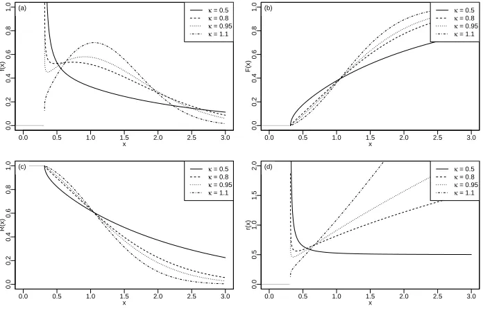
Figure 1. Plots of the GRay(γ = 0.1, κ, λ = 1) for different values of κ: (a) PDF, (b) CDF, (c) reliability function and (d) failure rate function.
where γ >0, κ >0 and λ >0. From Equation (2.1) it is easy to show that the cumulative distribution function (CDF) is given by
F(x) = 1−exp
−λ(x
2−γ)κ 2
, x >√γ, (2.2)
the reliability, or survivor, function by
R(x) = 1−F(x) = exp
−λ(x
2−γ)κ 2
, x >√γ, (2.3)
and the failure rate function by
r(x) = f(x)
R(x)=λ κ x(x
2−γ)κ−1, x >√γ. (2.4)
The behaviour of the density function, cumulative distribution function, failure rate function and the reliability function is shown in Figure (3). These functions shift left and right asγ changes, and there is a scale change in the x-direction as
λchanges, but there are more profound changes withκ. Here, these figures have fixedγ= 0.1 andλ= 1.0, butκis selected to illustrate different shapes.
Note that the derivative of the failure rate function, in Equation (2.4), is
∂r(x)
∂x =λκ(x
This derivative depends on all three parameters λ, γ and κ, but the shape only changes asκ changes. Forκ≥ 1, one can show that (2κ−1)x2−γ > 0 for all values ofx, and this shows thatr(x) is an increasing function. For 0< κ≤0.5, then (2κ−1)x2−γ <0 and this shows thatr(x) is a decreasing function. Finally,
for 0.5< κ <1, then (2κ−1)x2−γ <0 or (2κ−1)x2−γ >0 based on the value
ofx, sor(x) has a bathtub shape. The examples in Figure 3 cover these types. Also, the quantile function,Q(q), can be found by solvingF(Q) =q, that is
1−exp
−λ(Q
2−γ)κ 2
=q
which leads to the result
Q(q) =
s
2
λln
1
1−q
1/κ
+γ, 0≤q≤1. (2.6)
Finally, note that values from theGRaydistribution can be simulated using the probability integral transformation approach, using Equation (2.6), to give
x= s 2 λln 1 1−U
1/κ
+γ, where U ∼Uniform(0,1). (2.7)
2.2. Summary measures. The statistical properties play an important role in the characterization of any distribution. Now some statistical properties of the GRay(γ, κ, λ) are considered.
Mean: To derive the mean of theGRay(γ, κ, λ), consider the definition
µ= E(X) = [−xR(x)]∞√
γ+
Z ∞
√
γ
R(x)dx. (2.8)
After making the substitutiony= (x2−γ)k, then Equation (2.8) becomes
µ=√γ+ 1 2κΓ
1 2κ 2 λ 2κ1 + 1 2κ ∞ X i=1 −1 2 i
γiη, (2.9)
whereη= Γ
1 2κ−
i κ
2
λ
2κ1−
i κ
.
Variance: Similarly, to find the variance, we have
E(X2) =γ+ 2
Z ∞
√
γ
xexp
−λ(x
2−γ)κ 2
dx, (2.10)
which, using the substitutiony= (x2−γ)κ, can be put in the form
E(X2) =γ+1
κ
Z ∞
0
yκ1−1exp
−λ
2y
dy,=γ+1
κΓ 1 κ 2 λ 1κ . (2.11)
From Equations (2.8) and (2.11), the variance ofGRay(γ, κ, λ) is given by
Var(X) =γ+1
κΓ 1 κ 2 λ 1κ − √
γ+ 1 2κΓ
1 2κ 2 λ 2κ1 + 1 2κ ∞ X i=1 −1 2 i
γiη
2
,
where, as above,η= Γ
1 2κ−
i κ
2
λ
2κ1−κi
.
Mode: The mode, forκ≥1, is found by equating ∂x∂ lnf(x) to zero. This leads to the mode being the solution of the following non-linear equation
1
x+ κ−1
x2−γ(2x)−λκx(x
2−γ)κ−1= 0. (2.13)
This cannot be solved explicitly and hence numerical methods must be used. For other values ofκ, the mode is at the far left, that is atx=√γ.
Median: The median can simply be found from the quantile function, Equation (2.6), withq= 12 and hence the median is given by
Median(X) =
s
2
λln(2)
1/κ
+γ. (2.14)
Mean residual life time: Letm(t) denotes the mean residual life time ofGRay(γ, κ, λ), then
m(t) = 1
R(t)
Z ∞
t
R(x)dx, (2.15)
which can be put in the following form
m(t) =
Z ∞
√
γ exp
Z t+x
t
r(y)dy
dx, (2.16)
see [26]. Note that forκ≥1, sincer(x) is increasing, thenm(t) is decreasing, for 0 < κ ≤0.5, since r(x) is decreasing, then m(t) is increasing. Finally, for r(x) first decreasing and then starting to increase monotonically at some timex, means thatm(t) is increasing and then decreasing.
3. Recurrence equations of upper record value moments
In this section some recurrence relations for the single and product moment and the moment generating function of upper record values from theGRaydistribution are stated. Using these recurrence relations, theGRaydistribution is characterized.
Theorem 3.1. Single moments of the upper record values: Recurrence relation for single moments of the upper record values fromGRaydistribution is defined in the following theorem.
Forn= 1,2, . . . andr= 1,2, . . .we have that
µrn+2+1=
1 +r+ 2 2κn
µrn+2−r+ 2
2κnγµ
r
n, (3.1)
whereµs l =E(X
S U(l)).
(1) Form= 1,2, . . . andr, s= 1,2, . . .
1 + 2κm
r+ 2
µrm,m+2,s+1=γµr,sm,m+1+ 2κm
r+ 2µ r+s+2
m+1 . (3.2)
(2) For1≤m≤n+ 1andr, s= 1,2, . . .
µrm+2+1,s,n=
1 +r+ 2 2κm
µrm,n+2,s−r+ 2
2κmµ
r,s
m,n, (3.3)
whereµl1,l2
m,n =E(X l1
U(m)X
l2
U(n)).
Theorem 3.3. Single moment generating function: Recurrence relation for single moment generating function of the upper record values formGRay(γ, κ, λ)is given by
Forn= 1,2, . . .
Mn+1(t) =− t
2κnδ 0
n(t) +
γt2
2κn+ 1
Mn(t)−tδn(t) +tδn+1(t), (3.4)
whereMl(t) =E(etXu(l)),δl(t) = d
dtMl(t), andδ
0
l(t) = d2
dt2Ml(t)).
Theorem 3.4. Joint moment generating functions: Recurrence relation for joint moment generating function of the upper record values form GRay distribution is stated.
Forn, m= 1,2, . . .
t21Mn,m00 (t1, t2) =(2κm+γt21)Mn,m(t1, t2)−2κmt1Mn,m0 (t1, t2)
+ 2κmt1Mn,m0 +1(t1, t2)−2κmMn,m+1(t1, t2), (3.5)
where Mn,m(t1, t2) is the joint moment generating function of XU(n),XU(m)
re-spectively, then
Mn,m(t1, t2) =E(et1XU(n)+t2XU(m)).
4. Maximum likelihood analysis
In this section, we estimateγ,κandλ, using maximum likelihood and compute the observed Fisher information. Suppose thatx={xU(1), xU(2), . . . , xU(n)}are the
first nupper record values from GRay(γ, κ, λ). The general form for a likelihood function for observed record valuesx, given by [1], is defined as
l(γ, κ, λ|x) = n−1
Y
i=1
f(xU(i))
1−F(xU(i))
f(xU(n)), (4.1)
where f(·) and F(·) are given by Equations (2.1) and (2.2), respectively. Then, substituting from Equations (2.1) and (2.2) into (4.1) gives
l(γ, κ, λ|x) =
λnκnexp
−λ(x
2
U(n)−γ)
κ
2
×Qn
i=1xU(i)(x2U(i)−γ)
κ−1,
ifxU(1)<
√
γ
0, otherwise.
The logarithm of the, non-zero part of the, likelihood function in Equation (4.2), that is whenxU(1)<
√
γ, gives the log-likelihood function
L(γ, κ, λ|x) =nlogλ+nlogκ−λ(x
2
U(n)−γ)
κ
2
+ n
X
i=1
(κ−1) log(x2U(i)−γ) + n
X
i=1
logxU(i). (4.3)
Notice that this is monotonic increasing inγ and hence the maximum will occur at a boundary of the parameter space for γ, and in particular ˆγ =xU(1) that is
the minimum of the record value sample. The maximum likelihood estimate of the other two parameters can be found by differentiating Equation (4.3) with respect to κand λand equating the results to zero. This leads to the normal equations for the parameters as
ˆ
λκˆ(x2U(n)−γˆ)ˆκ−1
2 −
n
X
i=1
ˆ
κ−1
x2
U(i)−ˆγ
= 0, (4.4)
and
n
ˆ
κ−
ˆ
λ
2(x
2
U(n)−ˆγ) ˆ
κlog(x2
U(n)−γˆ) + ˆκ
n
X
i=1
log(x2U(i)−γˆ) = 0. (4.5)
The MLEs ofκandλcan be obtained by simultaneously solving Equations (4.4) and (4.5). However, since Equations (4.4) and (4.5) cannot be solved analytically some numerical method is needed—here the optim function in R [20] has been used.
In general, the asymptotic variances and covariances of the MLE for parameters, θ = (θ1, θ2) say, are given by elements of the inverse of the (expected) Fisher
information matrix, I, whereas an approximate variance-covariance matrix, Σn, can be obtained from the observed information matrix,In. That is,
Σ =
Var(ˆθ1) cov(ˆθ1,θˆ2)
cov(ˆθ1,θ2ˆ ) Var(ˆθ2)
≈ −In−1( ˆθ) (4.6)
where
In( ˆθ) =
∂2L(θ)
∂θ2 1
∂2L(θ)
∂θ1∂θ2
∂2L(θ)
∂θ1∂θ2
∂2L(θ)
∂θ2 2
θ= ˆθ
. (4.7)
The asymptotic normality of the MLEs, subject to the usual regularity condi-tions, can be used to compute the approximate confidence intervals forθ1 andθ2.
Therefore, (1−α)100% confidence intervals are, respectively,
θ1±zα/2sd(ˆθ1), θˆ2±zα/2 sd(ˆθ2)
where sd(·) is the standard deviation of the argument andzα/2is the percentile of
the standard normal distribution with right-tail probability equal toα/2.
θ2,
2L( ˆθ)−L(θ1,θˆ2)∼χ2d (4.8)
whereL( ˆθ) is the log-likelihood function of the full maximum likelihood estimates, whereas L(θ1,θˆ2) is the log-likelihood function evaluated with fixed parameters
θ1, and degrees of freedomd is the number of parameters inθ1. To construct a Wilks confident interval, or region, this can be re-arranged to give
θ1:L(θ1,θˆ2)≥L( ˆθ)−1
2χ
2
d
. (4.9)
Particular cases are, for example, the 1D confidence interval for θ1 = κ giving
d= 1, withθ2= (γ, λ), and the 2D confidence region forθ1= (κ, λ) givingd= 2,
withθ2=γ.
Note that although these results can be applied forκandλ, the non-regularity forγmeans that an alternative is required. In particular, here the highest density 95% confidence interval for ˆγ, denoted as (ˆγL,ˆγU), can be calculated using the fact that ˆγU = ˆγ =x2U(1) and where ˆγL is such that P r(ˆγ ≥ ˆγL) = 0.95. Note that sincex2
U(1) =x 2
1 with, x1 ∼GRay, the density of ˆγ is a simple transformation of
theGRayPDF and hence the value ˆγL can be found easily.
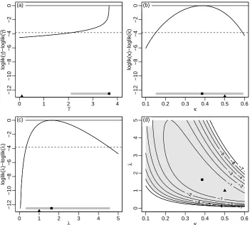
To illustrate maximum likelihood estimation consider Figure 2 which uses a record value dataset of sizen= 5 from aGRay(γ= 0.1, κ= 0.5, λ= 1) distribution. In each of (a)–(c), the profile log-likelihood is shown as a bold curve, showing that ˆ
γis located at the boundary of the parameter space whereas the other parameter estimates occur at turning points. The location of estimated values are shown with a black square and the true values as black triangles. Also shown for each is a confidence interval as a grey bar which has been calculated using the Wilks confidence interval/region result. A bivariate confidence region for (κ, λ) is shown in (d) superimposed on the 2D log-likelihood surface contours.
5. Bayesian estimation
This section describes Bayesian modelling of record values from theGRay(γ, κ, λ) distribution with the MCMC algorithm described in the next section. The main idea of the Bayesian approach and computational implementation with MCMC algorithms is to generate samples from the posterior density function and then to compute the Bayes point estimates and also construct the corresponding credible intervals based on the generated posterior samples. By considering theGRaymodel in Equation (2.1), assume the following gamma prior densities forγ,κandλwith parameters (α1, β2), (α2, β2) and (α3, β3) as follows, starting withγ,
π(γ|α1, β1) = γ α1−1
Γ(α1)βα1
1
exp
− γ
β1
, γ >0;α1, β1>0, (5.1)
then forκ,
π(κ|α2, β2) = κ α2−1
Γ(α2)βα2
2
exp
− κ
β2
0 1 2 3 4
−12
−10
−8
−6
−4
−2
0
γ
loglik(
γ
)−loglik(
γ
^)
(a)
0.1 0.2 0.3 0.4 0.5 0.6
−12
−10
−8
−6
−4
−2
0
κ
loglik(
κ
)−loglik(
κ
^)
(b)
0 1 2 3 4 5
−12
−10
−8
−6
−4
−2
0
λ
loglik(
λ
)−loglik(
λ
^ )
(c)
κ
λ
0.1 0.2 0.3 0.4 0.5 0.6
0
1
2
3
4
[image:9.612.127.478.118.434.2]5 (d)
Figure 2. Illustration of maximum likelihood estimation show-ing the profile likelihood functions for: (a) γ, (b) κ, and (c) λ, and in (d) the bivariate profile likelihood forκandλ. In each, the black square marks the MLE with true value marked as a black triangle, and the grey interval or region shows the approximate 95% confidence interval/region.
and finally forλ,
π(λ|α3, β3) = γ α3−1
Γ(α3)βα3
3
exp
− λ
β3
, γ >0;α3, β3>0. (5.3)
Now, assumingγ,κandλare independent, then the joint prior density ofγ,κ
andλcan be written as
π(γ, κ, λ) =π(γ|α1, β1)π(κ|α2, β2)π(λ|α3, β3)
= γ
α1−1κα2−1λα3−1
Γ(α1)βα1
1 Γ(α2)β
α2
2 Γ(α3)β
α3
3
×exp
−
γ
β1 + κ β2 +
λ β
This approach follows that of [7], with the assumption that the parameter prior distributions are gamma distribution as suggested by [13]. Note that the hyper-prior parameters, (α1, β2), (α2, β2) and (α3, β3), can be fixed based on expert knowledge or via information from separate calibration experiments. An example of the former is that an expert might be able to provide a mean and variance for a parameter, say mand v. Then, as the expectation of the gamma distribution takes form E(θ) =αβ, and variance Var(θ) =αβ2, the corresponding hyper-prior
parameters can be taken as α=m2/v and β =v/m. We have chosen values of α1=α2=α2= 1 andβ1= 1/10,β2=β3= 1, as arbitrary values, but particular applications will lead to other choices. In early experimentation, it was found that the only important choice was the value ofβ1where a prior favouring small values is very worthwhile. Moderate change in the other values has negligible influence on the estimation.
Based on the likelihood function of the observed sample given in Equation (4.2) and the joint prior in Equation (5.4), then the joint posterior density ofγ, κand
λ, given the data, is given by
π(γ, κ, λ|x) = R∞ l(γ, κ, λ|x)π(γ, κ, λ) 0
R∞
0
R∞
0 l(γ, κ, λ|x)π(λ, γ, k)dγ dκ dλ
. (5.5)
The Bayes estimator of any function of the parametersγ,κandλ, sayg(γ, κ, λ), under squared error loss function, is
Eγ,κ,λ|x(g(γ, κ, λ)) =
R∞
0
R∞
0
R∞
0 g(γ, κ, λ)l(γ, κ, λ|x)π(γ, κ, λ)dγ dκ dλ
R∞
0
R∞
0
R∞
0 l(γ, κ, λ|x)π(γ, κ, λ)dγ dκ dλ
. (5.6)
Evaluating the ratio of the two integrals in Equation (5.6) is too complex and complicated, and hence in this case the MCMC method is proposed to generate samples from the posterior distributions and then compute an approximation to the exact Bayes estimate ofg(γ, κ, λ).
The important aspects of the joint posterior are obtained by multiplying the likelihood and the joint prior of γ, κ and λ, as the normalising constant has no information about the unknown parameters, hence the following statement highlights the key structure,
π(γ, κ, λ|x)∝l(γ, κ, λ|x)π(γ, κ, λ) which in our particular case gives
= γ
α1−1kn+α2−1λn+α3−1
Γ(α1)βα1
1 Γ(α2)β
α2
2 Γ(α3)β
α3
3
×exp
−
γ β1 +
k β2 +
λ β3
exp
−λ(x
2
U(n)−γ)
k
2
×
n
Y
i=1
xU(i)(x2U(i)−γ)
k−1. (5.7)
6. The Metropolis-Hastings method
The estimation of the parameters is based on the approximate posterior distri-bution computations using a standard Metropolis-Hastings (M-H) algorithm. This is a special case of the Markov chain Monte Carlo (MCMC) approach, whose use has become widespread in the general statistical literature. The M-H algorithm is the first example of a MCMC approach used for parameter estimation and was proposed by [16] and subsequently generalized by [11]. Use of such methods for parameter estimation, and general density exploration, is widespread; a review can be found in [23], and for theoretical details see [8], [15] and [4]. For general practical examples see the collection by [10].
The Markov chain can start at any feasible point in the parameter space, let this arbitrary value be denotedθ0. From this starting point a discrete time Markov
chain is simulated to produce values,θ1,θ2, . . . ,θK say. The algorithm used here is defined as a single-variable random walk MCMC algorithm, see for example [2]. It is one of the simplest schemes, but works well for many applications. It is based on a random walk and uses separate single variable updates. That is, at each step only the value of a single variable is proposed and the proposal is a perturbation of the current value with variance parameter chosen to achieve an acceptable con-vergence rate. This proposed value is accept with a probability which depends on the posterior distribution. The general structure of the algorithm is given by
(1) Set an initial value forθ={γ, κ, λ}, call thisθ0. (2) Repeat the following steps fork= 1, . . . , K.
Fori = 1,2,3, that is for each parameters, θ = (θ1, θ2, θ3) = (γ, κ, λ), in turn.(a) Generate a propose new valueθi∗=θik+where∼N(0, τi2).
(b) Evaluate an acceptance probabilityα, as detailed below. (c) Generateufrom a uniform distribution,U(0,1).
(d) Ifα > u then accept the proposal and setθki =θi∗, elseθki =θki−1. End
End Repeat
The components ofθare of the different types,γ,κandλ, each allowing different simplifications of the acceptance probability in Step 2(b) above. To explain this, each type will now be considered separately.
Updates of γ: A proposed new value γ0 of parameter γ is drawn from normal distribution centred on the current parameter value, with variance τ12, chosen to
achieve an acceptable convergence rate. Here proposals which are negative or greater than the minimum of the squared data values are rejected, but otherwise the proposal is accepted with probability
α(γ0, γ) = min
1,l(γ
0, κ, λ|x)π(γ0) l(γ, κ, λ|x)π(γ)
,
otherwise it is rejected and no change is made.
Updates of κ: A proposed new value κ0 of parameter κ is drawn from normal distribution centred on the current parameter value, with variance τ2
2, chosen to
if positive the proposal is accepted with probability
min
1,l(γ, κ
0, λ|x)π(κ0) l(γ, κ, λ|x)π(κ)
,
otherwise it is rejected and no change is made.
Updates of λ: A proposed new value λ0 of parameter λ is drawn from normal distribution centred on the current parameter value, with variance τ32, chosen to achieve an acceptable convergence rate. Here negative proposals are rejected, but if positive the proposal is accepted with probability
min
1,l(γ, κ, λ
0|x)π(λ0) l(γ, κ, λ|x)π(λ)
,
otherwise it is rejected and no change is made.
It is important to realise that both low and high values of τ12, τ22 and τ32, lead to long transient periods and highly correlated samples and hence unreliable estimation [2]. A reasonable proposal variance can usually be chosen adaptively during the early burn-in period, and it has been shown that for a wide variety of problems an acceptance rate of about 20%−30% is reasonable [24]. A judgement of when to declare convergence to the equilibrium distribution, and assessment of the efficiency of the algorithm can be made using sample path trace plots and autocorrelation functions. Also, required sample sizes can be calculated (see for example, [2]).
Once the sample has been generated from the posterior distribution, a number of possible estimators are available. After re-labelling, let θ1,θ2, . . . ,θN be the MCMC sample collected after the equilibrium of the Markov chain has been de-clared, then the posterior mean and variance, for a particular parameterθ, can be estimated by the corresponding sample mean and variance:
b
θ= ¯θ= 1
N
N
X
k=1
θk, bσ2= 1
N−1 N
X
k=1
(θk−θ¯)2.
In some cases, for example with very skew distributions or with small sample sizes, it is better to use more robust estimators, such as the posterior median and percentile-based credible intervals. These can easily be obtained by first ordering the sampled values to giveθ(1), θ(2), . . . , θ(N), whereθ represents any ofγ,κand λ. Then the posterior median estimate is given by
ˆ
θ=θ(N/2) (6.1)
Similarly, the 100(1−α)% credible interval forθis given by
θ(N α/2), θ(N(1−α)/2)
.
To calculate an approximate MAP estimate, the MCMC algorithm could be converted into a simulated annealing algorithm [9]. In particular a temperature,
Tk, is included, which decreases as the iterations progress, withTk= 2/log(1 +k) being one choice of annealing schedule. Hence, the acceptance ratio,α, is replaced
byαTk. Note that, the MAP estimate is taken as the final iteration, b
θMAP=bθ
The advantage of simulated annealing is that it provides an answer more quickly than a sampling algorithm. On the other hand, the disadvantage is that it does not produce a posterior sample for further investigation [2].
7. Experiments
7.1. Preliminaries. To evaluate the behaviour of the proposed distribution, dif-ferent upper record value samples from the GRay distribution are simulated and estimates are calculated using the maximum likelihood and Bayesian methods al-ready described. All graphs and calculations have been produced in R[20], with code scripts available from the authors.
To generate a dataset of record values, consider the following sequence of values (to 2dp) from theGRay(0.1,0.5,1.0) distribution.
0.87 0.64 2.26 2.17 3.81 0.48 1.83 1.69 3.22 1.76
7.16 0.96 0.55 1.45 4.08 4.03 2.84 0.37 0.67 3.92 1.89 0.35 9.20 1.85 1.14 1.38 1.91 0.49 1.59 4.04
Those in bold correspond to the record values for a dataset of n = 5, that is
U(1) = 1 with xU(1) = 0.87, U(2) = 3 withxU(2) = 2.26, U(3) = 4 withxU(3) =
3.81, U(4) = 11 with xU(4) = 7.16, U(5) = 23 with xU(5) = 9.20, giving x =
(0.87,2.26,3.81,7.16,9.20).
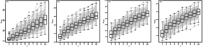
Throughout the simulation study γ = 0.1 and λ= 1 as these do not have an effect on the distribution shape, but the valuesκ= 0.5,0.8,0.95 and 1.1, defined as Cases 1–4, as in Figure 2, are considered as representative. Figure 3 shows a summary of M = 100 record value datasets, each of size n = 10. In each, the grey lines link together the data values within the same dataset. Note that the variability increases with n, as well as the mean, and that there is considerable overlap between boxplots. Also, the values are considerably greater in (a), the case withκ= 0.5, compared to the others.
● ● ● ● ● ● ● ● ● ● ● ● ●
1 2 3 4 5 6 7 8 9 10
0
10
20
30
xU(
n ) ● ● ● ● ● ● ● ● ● ● ● ● ●
1 2 3 4 5 6 7 8 9 10
0
10
20
30
n
xU(
n ) (a) ● ● ● ● ● ● ● ● ● ● ● ● ● ●
1 2 3 4 5 6 7 8 9 10
0
2
4
6
8
xU(
n ) ● ● ● ● ● ● ● ● ● ● ● ● ● ●
1 2 3 4 5 6 7 8 9 10
0 2 4 6 8 n
xU(
n
)
(b)
● ●
1 2 3 4 5 6 7 8 9 10
1 2 3 4 5 6 7
xU(
n
)
● ●
1 2 3 4 5 6 7 8 9 10
1 2 3 4 5 6 7 n
xU(
n ) (c) ● ● ● ●
1 2 3 4 5 6 7 8 9 10
1
2
3
4
5
xU(
n
)
● ● ●
●
1 2 3 4 5 6 7 8 9 10
1 2 3 4 5 n
xU(
n
)
[image:13.612.127.481.460.543.2](d)
Figure 3. Boxplots of record value data, with n = 10, from GRay(γ= 0.1, κ, λ= 1) for different values ofκwhere each box-plot containsM = 100 values and values in the same dataset are linked by a grey line: (a)κ= 0.5, (b)κ= 0.8, (c) κ= 0.95, (d)
κ= 1.1.
estimates, asymptotic confidence intervals and Bayesian posterior median with posterior 95% credible interval forγ,κandλare calculated.
7.2. Maximum likelihood results. A collection ofM = 100 replicates are used to compute different estimates of λ, γand κwith results summarised in Table 1. Recall that in all Cases the true valuesγ= 0.1 and λ= 1.0 are used, but that in: Case 1κ= 0.5; Case 2κ= 0.8; Case 3κ= 0.95; and Case 4 κ= 1.1.
Case 1 Case 2 Case 3 Case 4
n= 5 n= 10 n= 5 n= 10 n= 5 n= 10 n= 5 n= 10
Maxim
um
lik
eliho
o
d
estimation
ˆ
γ 6.36 9.88 2.65 3.18 1.94 2.46 1.73 2.08
Bias 6.26 9.78 2.55 3.08 1.84 2.36 1.63 1.98
SD 10.14 16.53 3.05 3.70 1.80 2.42 1.62 1.79
RMSE 11.87 19.14 3.96 4.80 2.57 3.38 2.29 2.66
Coverage 0.96 0.89 0.77 0.77 0.71 0.69 0.67 0.58 ˆ
κ 0.34 0.40 0.41 0.52 0.44 0.56 0.46 0.60
Bias -0.16 -0.10 -0.39 -0.28 -0.51 -0.39 -0.64 -0.50
SD 0.07 0.08 0.07 0.09 0.07 0.09 0.08 0.10
RMSE 0.18 0.13 0.40 0.29 0.51 0.40 0.65 0.51
Coverage 0.67 0.59 0.33 0.19 0.26 0.07 0.13 0.02 ˆ
λ 2.38 2.12 3.63 3.17 4.27 3.79 4.89 4.43
Bias 1.38 1.12 2.63 2.17 3.27 2.79 3.89 3.43
SD 0.92 1.04 0.96 1.20 1.11 1.25 1.98 1.29
RMSE 1.66 1.52 2.80 2.48 3.45 3.06 4.36 3.66
[image:14.612.131.452.512.653.2]Coverage 0.98 0.81 0.84 0.44 0.69 0.26 0.58 0.11
Table 1. Summary results forγ, κandλobtained using MLE,
averaged overM = 100 replicates.
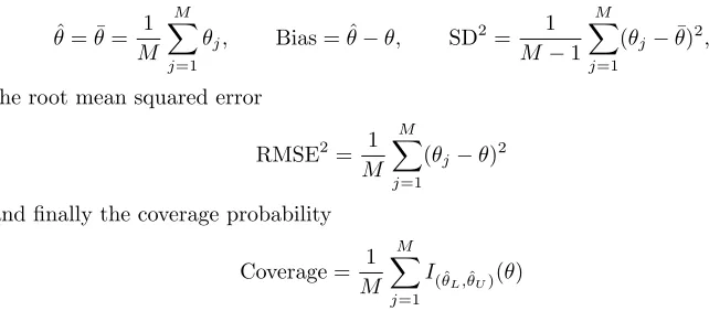
For each replicated data set a triplet of parameter estimates are obtained, pro-ducing the complete set ˆγj, ˆκj, ˆλj, for j = 1, . . . , M = 100. The results are then summarised using the following (referring to a general parameterθ): the mean of the estimates, corresponding bias and standard deviation of the estimates
ˆ
θ= ¯θ= 1
M
M
X
j=1
θj, Bias = ˆθ−θ, SD2= 1
M −1 M
X
j=1
(θj−θ¯)2,
the root mean squared error
RMSE2= 1
M
M
X
j=1
(θj−θ)2
and finally the coverage probability
Coverage = 1
M
M
X
j=1 I( ˆθ
L,θˆU)(θ)
where indicator functionI( ˆθ
L,θˆU)(θ) = 1 ifθ∈(ˆθL,
ˆ
In all cases the estimation is poor with the key issue regarding the estimation ofγwhich has a knock-on effect onκandγ – recalling that ˆγ=x2U(1) that is the first record value. As with other non-regular situations, this is a biased estimator and in some cases has produced a very substantial error.
7.3. Bayesian estimation results. The sameM = 100 replicates are used to compute estimates of λ, γ and κ using the posterior median and posterior 95% credible intervals, as defined in Section 5, with results summarised in Table 2. Recall, again, that in all Cases the true valuesγ= 0.1 andλ= 1.0 are used, but that in: Case 1 κ= 0.5; Case 2 κ= 0.8; Case 3 κ= 0.95; and Case 4 κ= 1.1. Typical final proposal standard deviations are 0.2972, 0.4493 and 1.2440 for γ, κ
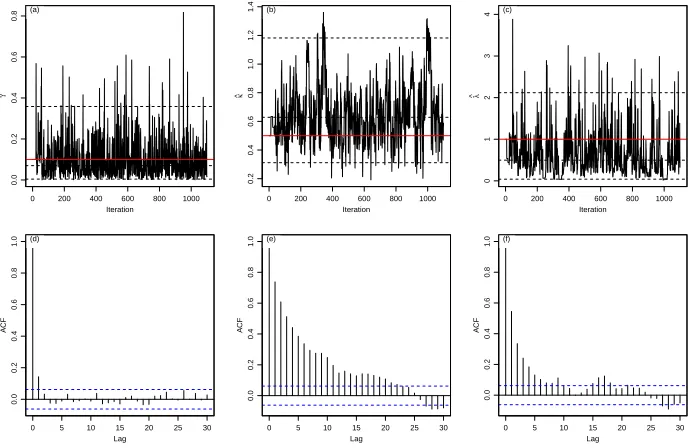
andλrespectively. The Markov chain paths, see the examples in Figures 4(a)–(c), show rapid convergence with no discernible trend and good random fluctuations. An initial 100 iterations have been discarded as burn-in, with the remainingM = 1000 forming the output sample. Similarly, the autocorrelations function in (d)– (f) show acceptable autocorrelation, although this is more borderline in the case ofκin (e). Declaring equilibrium after 100 iterations, the remainder of the sample is used for estimation. The results of the sample size calculations suggested that 63, 587 and 283 iterations are sufficient for the main run, and hence the actual 1000 is more than adequate.
0 200 400 600 800 1000
0.0
0.2
0.4
0.6
0.8
Iteration
γ
^
(a)
0 200 400 600 800 1000
0.2
0.4
0.6
0.8
1.0
1.2
1.4
Iteration
κ
^
(b)
0 200 400 600 800 1000
0
1
2
3
4
Iteration
λ
^
(c)
0 5 10 15 20 25 30
0.0
0.2
0.4
0.6
0.8
1.0
Lag
A
CF
Series params[(nburn + 1):M, p]
(d)
0 5 10 15 20 25 30
0.0
0.2
0.4
0.6
0.8
1.0
Lag
A
CF
Series params[(nburn + 1):M, p]
(e)
0 5 10 15 20 25 30
0.0
0.2
0.4
0.6
0.8
1.0
Lag
A
CF
Series params[(nburn + 1):M, p]
[image:15.612.131.476.365.589.2](f)
Figure 4. Monitoring traces and autocorrelation function gen-erated by the MCMC method.
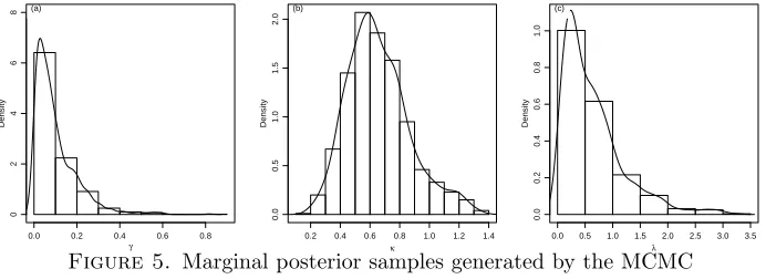
concentration around the true value ofκ= 0.5. In (c), again the distribution is skew with many values below the trueλ= 1.0. Overall, these figures indicate that good estimation should be possible, but that all distributions are skew and hence the use of the robust estimators is advisable compared to the more conventional means and variances.
γ
Density
0.0 0.2 0.4 0.6 0.8
0
2
4
6
8 (a)
κ
Density
0.2 0.4 0.6 0.8 1.0 1.2 1.4
0.0
0.5
1.0
1.5
2.0
(b)
λ
Density
0.0 0.5 1.0 1.5 2.0 2.5 3.0 3.5
0.0
0.2
0.4
0.6
0.8
1.0
[image:16.612.132.478.192.318.2](c)
Figure 5. Marginal posterior samples generated by the MCMC
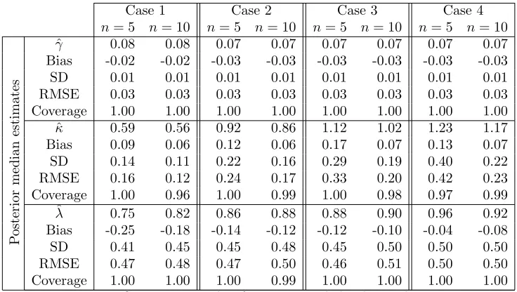
method summarised using histograms and kernel density curves.
Numerical results are summaries in Table 2 based on posterior median and posterior 95% credible intervals. As with the maximum likelihood estimation, each data produces a triplet of parameter estimates with the results summarised using: the mean estimates, bias, standard deviation, the root mean squared error, and the coverage probability. It is clear that all estimation is now substantial better than with maximum likelihood. In particular biases and RMSE are low with good coverage. There is a slight improvement due to the larger sample size, except forγwhere there is no change. Recall that in all Cases the true values for
γ andλare fixed, but that in: Case 1 κ= 0.5; Case 2κ= 0.8; Case 3κ= 0.95; and Case 4κ= 1.1. In all Cases, there is little change in the estimation properties forγandλ, but some changes forκ. Overall, now the estimation is very good and hence the inclusion of prior information has been very successful.
8. Summary
In this paper, a new distribution has been proposed with many theoretical prop-erties derived or stated. Methods for parameter estimation from record value data has been developed using the maximum likelihood and Bayesian approaches. In both, care had to be taken because of the non-regular nature of one parameter, and because of non-symmetrical and in particular non-Gaussian parameter sam-pling distributions. The maximum likelihood approach has been shown to work very badly, but in contrast the proposed Bayesian modelling linked with MCMC estimation has worked very well. Although the Bayesian model included arbi-trarily chosen prior parameters the exact values are not overly influential on the results—clearly, a sensitivity analysis would be useful further work.
Case 1 Case 2 Case 3 Case 4
n= 5 n= 10 n= 5 n= 10 n= 5 n= 10 n= 5 n= 10
P
osterior
median
estimates
ˆ
γ 0.08 0.08 0.07 0.07 0.07 0.07 0.07 0.07
Bias -0.02 -0.02 -0.03 -0.03 -0.03 -0.03 -0.03 -0.03
SD 0.01 0.01 0.01 0.01 0.01 0.01 0.01 0.01
RMSE 0.03 0.03 0.03 0.03 0.03 0.03 0.03 0.03
Coverage 1.00 1.00 1.00 1.00 1.00 1.00 1.00 1.00 ˆ
κ 0.59 0.56 0.92 0.86 1.12 1.02 1.23 1.17
Bias 0.09 0.06 0.12 0.06 0.17 0.07 0.13 0.07
SD 0.14 0.11 0.22 0.16 0.29 0.19 0.40 0.22
RMSE 0.16 0.12 0.24 0.17 0.33 0.20 0.42 0.23
Coverage 1.00 0.96 1.00 0.99 1.00 0.98 0.97 0.99 ˆ
λ 0.75 0.82 0.86 0.88 0.88 0.90 0.96 0.92
Bias -0.25 -0.18 -0.14 -0.12 -0.12 -0.10 -0.04 -0.08
SD 0.41 0.45 0.45 0.48 0.45 0.50 0.50 0.50
RMSE 0.47 0.48 0.47 0.50 0.46 0.51 0.50 0.50
[image:17.612.125.493.114.322.2]Coverage 1.00 1.00 1.00 0.99 1.00 1.00 1.00 1.00
Table 2. Summary results for γ, κ and λ obtained using Bayesian analysis, averaged overM = 100 replicates.
for different applications. Therefore, the continued development of increasingly more flexible distributions allows the modelling of increasingly more complicated situations. The new generalized Rayleigh distribution proposed in this paper, can now be added to the array available to applied statisticians – and we hope that it will be further studied. Finally, the use of Bayesian modelling has been of great benefit and similar approaches are likely to be helpful in other situations also—this can be another areas of future study.
Acknowledgment. The authors thank the Editor and the anonymous referees for the helpful comments.
References
1. Arnold, B. C., Balakrishnan, N. and Nagaraja, H. N.: Records, John Wiley & Sons, 1998. 2. Aykroyd, R. G.: Statistical Image Reconstruction, inIndustrial tomography: Systems and
Applications, Woodhead Publishing, pp. 401–424, 2015.
3. Balakrishnan, N. and Cohen, A. C.: Order Statistics and Inference: Estimation Methods, Academic Press, 1991.
4. Brooks, S., Gelman, A., Jones, G. and Meng, X-L.: Handbook of Markov Chain Monte Carlo, Chapman and Hall/CRC, 2011.
5. Cohen, A. C. and Whitten, B. J.:Parameter Estimation in Reliability and Life Span Models, Marcel Dekker, 1988.
6. Dyer, D. D. and Whisenand, C. W.: Best linear unbiased estimator of the parameter of the Rayleigh distribution. Part I: Small sample theory for censored order statistics,IEEE Transactions on Reliability,22, 27–34, 1973.
8. Gamerman, D. and Lopes, H. F.: Markov Chain Monte Carlo: Stochastic simulation for Bayesian inference, 2nd Ed. Chapman and Hall/CRC, 2006.
9. Geman, S. and Geman, D.: Stochastic relaxation, Gibbs distributions, and the Bayesian restoration of images,IEEE Transactions on Pattern Analysis and Machine Intelligence 6, 721–741, 1984.
10. Gilks, W.R., Richardson, S. and Spiegelhalter, D.J.:Markov Chain Monte Carlo in Practice, Chapman and Hall/CRC, 1996.
11. Hastings, W.K.: Monte Carlo sampling methods using Markov Chains and their applications, Biometrika57, 97–109, 1970.
12. Hirano, K.: Some properties of the distributions of order k, Fibonacci Numbers and Their Applications42, 45–61, 1986.
13. Kim, C. and Han, K.: Bayesian estimation of Rayleigh distribution based on generalized order statistics,Applied Mathematics Sciences8, 7475–7485, 2014.
14. Lee, K.R., Kapadia, C.H. and Brock, D.B.: On estimating the scale parameter of the Rayleigh distribution from doubly censored samples,Statistische Hefte 21, 14–29, 1980.
15. Liu, J.S.: Monte Carlo strategies in scientific computing, Springer Science and Business Media, 2001.
16. Metropolis, N., Rosenbluth, A.W., Rosenbluth, M.N., Teller, A.H. and Telle, E.: Equation of state calculations by fast computing machines, The Journal of Chemical Physics 21, 1087–1092, 1953.
17. Miller, K.S. and Sackrowitz, H.: Relationships between biased and unbiased Rayleigh distri-butions,SIAM Journal on Applied Mathematics15, 1490–1495, 1967.
18. Miller, K.S.:Multidimensional Gaussian distributions, John Wiley & Sons Inc, 1964. 19. Polovko, A.M.:Fundamentals of reliability theory, Academic Press, 1968.
20. R Core Team,R: A language and environment for statistical computing, R Foundation for Statistical Computing, Vienna, Austria, 2016.
21. Lord Rayleigh, On the resultant of a large number of vibrations of the same pitch and of arbitrary phase,The London, Edinburgh, and Dublin Philosophical Magazine and Journal of Science10, 73–78, 1880.
22. : On the the problem of random vibrations and of random fights in one, two, or three distributions,Philosophical Magazine 37, 321, 1919.
23. Robert, C. and Casella, G.: A short history of Markov Chain Monte Carlo: Subjective recollections from incomplete data,Statistical Science26, 102–115, 2011.
24. Gelman, A., Gilks, W.R. and Roberts, G.O.: Weak convergence and optimal scaling of random walk Metropolis algorithms,The Annals of Applied Probability7, 110–120, 1997. 25. Sinha, S.K. and Howlader, H.A.: Credible and hpd intervals of the parameter and reliability
of Rayleigh distribution,IEEE Transactions on Reliability 32, 217–220, 1983.
26. Watson G.S. and Wells, W.T.: On the possibility of improving the mean useful life of items by eliminating those with short lives,Technometrics3, 281–298, 1961.
Robert G. Aykroyd: Department of Statistics, University of Leeds, Leeds, UK
E-mail address:[email protected]
M. A. W. Mahmoud: Department of Mathematics, Al-Azhar University, Cairo, Egypt
E-mail address:[email protected]
Hassan M. Aljohani: Department of Statistics, University of Leeds, Leeds, UK
E-mail address:[email protected]