Probabilistic Inference in Piecewise Graphical Models

Graphical Models

Hadi Mohasel Afshar

A thesis submitted for the degree of Doctor of Philosophy at The Australian National University

I hereby declare that this thesis is my original work which has been done in collab-oration with other researchers. This document has not been submitted for any other degree or award in any other university or educational institution. Parts of this thesis have been published in collaboration to other researchers in international conferences as listed below:

• (Chapter 4) H. M. Afshar, S. Sanner, and E. Abbasnejad (2015). Linear-time Gibbs Sampling in Piecewise Graphical Models. In Proceedings of the 29th AAAI Conference on Artificial Intelligence (AAAI-15), Austin, U.S.

• (Chapter 5) H. M. Afshar, S. Sanner, C. Weber (2016). Closed-form Gibbs Sam-pling for Graphical Models with Algebraic Constraints, The 30th AAAI Confer-ence on Artificial IntelligConfer-ence, Phoenix, U.S.

• (Chapter 6) H. M. Afshar and J. Domke (2015). Reflection, Refraction and Hamiltonian Monte Carlo, The 29-th Conference on Neural Information Pro-cessing Systems (NIPS-15), Montreal, Canada.

Hadi Mohasel Afshar 2 August 2016

I would like to express my gratitude towards all who helped me make this thesis possible.

First and foremost, I would like to thank my supervisorScott Sanner for his in-sightful guidance throughout my PhD, for his caring and patience in introducing me to the field of graphical models, for his intuitive advice about the potentially fruitful lines of research, for all invaluable discussions I had with him and all I learned from him but above all, for his friendship, support and encouragement through the tough-est times. I have been quite lucky to have a supervisor that was more concerned about his students and their future than the students would care about themselves and their own future. I am extremely grateful for all these and feel deeply in dept.

I would like to thank the chair of my supervisory panel Prof. Marcus Hutterfor teaching me how to think in a more disciplined way, how to formalize my intuitions and how to interpret formulas intuitively. I had the opportunity to learn from his sub-tle vision and enjoyed participating in his reinforcement reading group. I appreciate all the time and energy he spent for me throughout my PhD.

Special thanks to the brilliant researcherJustin Domke. I really enjoyed working with him and learned a lot from him.

I would like to thank my adviser Prof. John Lloyd, Prof Bob Williamson and Chris Webersfor their advice and the discussions that I had with them.

I acknowledge the financial, academic and technical support provided by the Aus-tralian National University (ANU) and appreciate the welcoming and collaborative environment provided by the National ICT of Australia (NICTA) where I had the op-portunity to work with talented researchers.

I would like to thank my fellow postgraduate friends. Special thanks to Firouzeh Khoshnoudi, Tom Everitt, Ehsan Abbasnejad, Phuong Nguyen, Mayank Daswani, Tor Lattimore, Jan Leike, Suvash Sedhain, Kar Wai, Paul Scott and many others for great discussions that we had and for making my life so joyful.

Finally I have to thank my parents from the depth of my heart for their endless love and support.

In many applications of probabilistic inference the models contain piecewise densities that are differentiable except at partition boundaries. For instance, (1) some mod-els may intrinsically have finite support, being constrained to some regions; (2) arbi-trary density functions may be approximated by mixtures of piecewise functions such as piecewise polynomials or piecewise exponentials; (3) distributions derived from other distributions (via random variable transformations) may be highly piecewise; (4) in applications of Bayesian inference such as Bayesian discrete classification and preference learning, the likelihood functions may be piecewise; (5) context-specific conditional probability density functions (tree-CPDs) are intrinsically piecewise; (6) influence diagrams (generalizations of Bayesian networks in which along with prob-abilistic inference, decision making problems are modeled) are in many applications piecewise; (7) in probabilistic programming, conditional statements lead to piecewise models. As we will show, exact inference on piecewise models is not often scalable (if applicable) and the performance of the existing approximate inference techniques on such models is usually quite poor.

This thesis fills this gap by presenting scalable and accurate algorithms for infer-ence in piecewise probabilistic graphical models. Our first contribution is to present a variation of Gibbs sampling algorithm that achieves an exponential sampling speedup on a large class of models (including Bayesian models with piecewise likelihood func-tions). As a second contribution, we show that for a large range of models, the time-consuming Gibbs sampling computations that are traditionally carried out per sam-ple, can be computed symbolically, once and prior to the sampling process. Among many potential applications, the resultingsymbolic Gibbs samplercan be used for fully automated reasoning in the presence of deterministic constraints among random vari-ables. As a third contribution, we are motivated by the behavior of Hamiltonian dy-namics in optics —in particular, the reflection and refraction of light on the refractive surfaces— to present a new Hamiltonian Monte Carlo method that demonstrates a significantly improved performance on piecewise models.

Hopefully, the present work represents a step towards scalable and accurate infer-ence in an important class of probabilistic models that has largely been overlooked in the literature.

Declaration iii

Acknowledgments vii

Abstract ix

1 Introduction 1

1.1 Motivation . . . 1

1.1.1 Bounded support models . . . 2

1.1.2 Mixture of truncated basis functions . . . 3

1.1.3 Random variable transformations . . . 4

1.1.4 Piecewise likelihoods . . . 5

1.1.5 Context-specific conditional densities . . . 7

1.1.6 Influence diagrams . . . 8

1.1.7 Probabilistic programming . . . 9

1.2 Contributions . . . 11

1.2.1 Gibbs sampling on piecewise models. . . 11

1.2.1.1 Linear time Gibbs sampling on piecewise models . . . . 11

1.2.1.2 Fully-automated symbolic Gibbs sampling on an ex-pressive family of piecewise models . . . 12

1.2.2 Hamiltonian Monte Carlo on piecewise models . . . 12

1.3 Thesis outline . . . 13

2 Probabilistic Graphical Models 15 2.1 Basic Definitions and Assumptions . . . 15

2.2 Representation of Graphical models . . . 18

2.2.1 Bayesian networks (BNs) . . . 18

2.2.1.1 Bayesian inference / Bayesian paradigm . . . 19

2.2.2 Markov random fields (MRFs) . . . 20

2.2.3 Factor graphs . . . 21

2.3 Inference in Graphical Models . . . 22

2.3.1 Exact inference . . . 23

2.3.1.1 Variable elimination (VE) . . . 24

2.3.1.2 Clustering (join tree) algorithms . . . 25

2.3.2 Approximate inference by sampling (Monte Carlo methods) . . . 27

2.3.2.1 Inverse transform sampling . . . 28

2.3.2.2 Forward sampling . . . 29

2.3.2.3 Rejection sampling . . . 30

2.3.2.4 Sampling by likelihood weighting (LW) . . . 32

2.3.2.5 Markov Chain Monte Carlo (MCMC) . . . 33

2.3.2.6 Metropolis-Hastings sampling (MH) . . . 34

2.3.2.7 Gibbs sampling . . . 37

2.3.2.8 Hamiltonian Monte Carlo (HMC) . . . 39

2.3.3 Other approximate inference methods . . . 44

2.3.3.1 Direct approximation of query . . . 45

2.3.3.2 Message passing based approximate inference . . . 45

2.4 Summary . . . 46

3 Piecewise Data Structures and Symbolic Operations 47 3.1 Piecewise functions . . . 47

3.1.1 C-piecewiseDfunction . . . 48

3.2 Piecewise Calculus . . . 49

3.2.1 Piecewise/non-piecewise operations . . . 49

3.2.2 Piecewise/piecewise elementary operations . . . 49

3.2.3 Maximum and Minimum . . . 50

3.2.4 Comparisons . . . 51

3.2.5 Substitution . . . 52

3.2.6 Integration . . . 52

3.3 Representation of piecewise functions . . . 54

3.3.1 Binary decision diagram (BDD) . . . 55

3.3.1.1 Reduced ordered binary decision diagram . . . 56

3.3.1.2 The canonicality of OBDDs . . . 56

3.3.2 Algebraic decision diagram (ADD) . . . 57

3.3.3 Extended algebraic decision diagram (XADD) . . . 57

3.3.4 Edge-valued decision diagrams . . . 58

3.3.4.1 Edge-valued BDD (EVBDD) . . . 59

3.3.4.2 Factored Edge-Valued BDD (FEVBDD) . . . 61

3.3.4.3 FDD, OFDD, BMD and *BMD . . . 61

3.3.4.4 Hybrid decision diagrams: OKFDD, KBMD, K*BMD, *PHDD . . . 61

3.3.4.5 Affine Algebraic Decision Diagrams . . . 62

3.4 Pruning piecewise functions and processing symbolic expressions . . . . 62

3.4.1 Computer Algebra Systems (CASs) . . . 63

3.4.2 Automated theorem-proving . . . 64

3.4.3 Satisfiability Modulo Theories (SMT) . . . 66

3.5 Summary . . . 68

4 Gibbs Sampling from augmented piecewise models 71 4.1 Case study I: Bayesian Pairwise Preference Learning (BPPL) . . . 72

4.2 Case study II: Bayesian Market Making (MM) . . . 75

4.4 Piecewise Models as Mixture Models . . . 77

4.4.1 Deterministic Dependencies and Blocked Sampling . . . 81

4.4.1.1 Blocked Gibbs . . . 81

4.4.1.2 Targeted Selection of Collapsed Auxiliary Variables . . 81

4.4.1.3 Convergence to the target distribution . . . 82

4.5 Experimental Results . . . 84

4.6 Conclusion . . . 86

5 Symbolic Gibbs Sampling in Algebraic Graphical Models 89 5.1 Introduction . . . 89

5.2 Momentum Model . . . 91

5.3 Stochastic-Deterministic graphical models . . . 92

5.3.1 Collapsing determinism (δ-collapsing) . . . 93

5.3.1.1 Proof of correctness . . . 95

5.3.1.2 Reconstructing eliminated variables . . . 97

5.3.2 Notes about the Dirac delta collapsing mechanism . . . 97

5.4 Polynomial Piecewise Fractionals (PPFs) . . . 99

5.4.1 Definition of a polynomial piecewise fractional function (PPF) . . 100

5.4.2 Some properties of the PPF family . . . 100

5.4.3 Analytic integration . . . 101

5.4.3.1 Analytic univariate PPF* integration . . . 101

5.5 Symbolic Gibbs Sampling . . . 103

5.6 Experimental Results . . . 104

5.6.1 Algorithms . . . 107

5.6.2 Measurements . . . 108

5.6.3 Experimental models . . . 109

5.6.4 Experimental evaluations . . . 112

5.7 Conclusion . . . 113

6 Reflective Hamiltonian Monte Carlo 115 6.1 Introduction . . . 115

6.2 Exact Hamiltonian Dynamics . . . 117

6.3 Reflection and Refraction with Exact Hamiltonian Dynamics . . . 118

6.4 Reflection and Refraction with Leapfrog Dynamics . . . 119

6.5 Volume Conservation . . . 122

6.5.1 Refraction . . . 122

6.5.2 Reflection . . . 125

6.5.3 Reflective Leapfrog Dynamics . . . 126

6.6 Experiment . . . 127

6.6.1 Sensitivity to parameter tuning . . . 129

6.6.2 The rate of rejections, reflections and refractions . . . 130

7 Conclusion 139 7.1 Summary of contributions . . . 139 7.2 Future work . . . 141 7.3 Conclusion . . . 144

Introduction

1.1

Motivation

Reasoning under uncertainty is an indispensable part of a large range of real-world application domains. In such inference tasks, it is required to predict the future state of the world and/or actions that lead to maximum gains based on some incomplete or uncertain information and partial/noisy observations. For instance, an optical character recognition system may encounter an ambiguous input glyph which can be mapped to more than one alphabet letter or a robot may requrie finding its goal given input signals received from its noisy sensors.

Statistical inference, based on probability theory, provides a natural and robust formalism for such reasoning tasks. The advent of graphical models (GMs) has (1) provided systematic methods to represent complex distributions in succinct and com-pact forms and (2) facilitated the extraction of structured information such as condi-tional dependencies of random variables. By exploiting such structures, GMs have (3) led to scalable and effective inference algorithms. Finally, by separating model repre-sentation from the inference, (4) GMs have enabled the users (e.g. data scientists) to focus on the design of appropriate models for the systems about which they intend to carry out inference while letting the actual reasoning task be performed by gen-eral and automated reasoning mechanisms. As a result, GMs have vastly expanded the application domains in which probabilistic reasoning can be effectively used and consequently, have become a fundamental model of machine learning and artificial intelligence.

Despite a relatively long history of probabilistic reasoning that can be traced back to sixteenth and seventeenth centuries [Hald 2003], for a long time, its use has been almost exclusively restricted to simple models which had closed-form solutions that could be worked out manually. Luckily, the rapid growth in the processing power of computers has changed the situation and led to the emergence of a range of ap-proximate inference algorithms that can handle a large range of models for which manual inference is intractable or impossible. In particular, particle-based algorithms –i.e. methods in which the original distribution is approximated by (a Markov chain of) samples– are appealing because they are asymptotically unbiased in the sense that if the number of sampled particles tends to infinity, the distribution approximation error tends to zero.

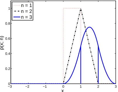
−30 −2 −1 0 1 2 3 0.2

0.4 0.6 0.8 1

x

p(x; n)

n = 1 n = 2 n = 3

Figure 1.1: Irwin-Hall probability density functions for parametern=1, 2, and 3.

However, the convergence rate of the particle based algorithms and in a broader view, the performance of all approximate inference methods can significantly depend on the characteristics of the original model. In particular, the performance of the existing approximate inference algorithms on piecewise models is often quite poor. Throughout, by piecewise models, we refer to models with probability density func-tions which are continuous and differentiable except at piecewise partition bound-aries. Such models have several applications.

In the remaining part of this subsection, we provide some pervasive application domains associated with models that are intrinsically piecewise.

1.1.1 Bounded support models

In many models, distributions have bounded support. As a result, some parametric distributions1that are extensively used in the literature are supported on semi-infinite intervals, such as the following:Beta prime, Chi, gamma and exponential distributions.

Some other well-known continuous distributions have bounded supports, such as:

Uniform, U-quadratic, beta, logitnormal, reciprocal, raised cosine, Von Mises, Kent, Wigner semicircle distributions, etc.

Finally, among bounded support distributions, some like the following are piece-wise with more than one segment:triangular, trapezoidal, Bates and Irwin-Hall distribu-tions.

To be more concrete, consider an Irwin-Hall distribution with parametern. This distribution is defined as follows:

p(x;n) = 1 2(n−1)!

n

∑

(−1)k

n k

(x−k)n−1sgn(x−k)

1_{Throughout, we often do not distinguish between distributions and density functions. The intention}

Therefore, p(x;n)is an(n+1)-piecewise function. For instance, Irwin-Hall distribu-tion with parametersn =1 to 3 are plotted in Figure 1.1. Clearly, p(x, 1)is a uniform distribution:

p(x; 1) =

(

1 if 0≤ x≤1 0 otherwise

p(x, 2)is a triangular distribution:

p(x; 2) =

      

x if 0≤ x≤1

2−x if 1< x≤2 0 otherwise

andp(x, 3)corresponds to a 4-piece distribution:

p(x; 3) =

           1

2x2 if 0≤x≤1 1

2 −2x2+6x−3

if 1<x≤2 1

2 x2−6x+9

if 2<x≤3

0 otherwise

1.1.2 Mixture of truncated basis functions

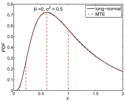
Piecewise exponential or polynomial functions (also known as mixtures of truncated polynomials and exponentials) are expressive enough to approximate arbitrary func-tions up to arbitrary precisions. For instance, following the approximation method used in [Cobb et al. 2006], Figure 1.2 shows that a log-normal distribution (with pa-rametersµ = 0 andσ2 =0.5) can be approximated by a 5-piece mixture of truncated exponentials (MTE) in a reasonably accurate manner. The corresponding MTE is as follows:                 

a01+a11exp b11(x−m)

+a21exp b21(x−m)

if exp(µ−3σ)≤x< d− a02+a12exp b12(x−m)

+a22exp b22(x−m)

ifd−≤ x<m a03+a13exp b13(x−m)

+a23exp b23(x−m)

ifm≤x <d+ a04+a14exp b14(x−m)

+a24exp b24(x−m)

ifd+≤ x<exp(µ+3σ)

0 otherwise

wherea∗∗andb∗∗are constants,m=exp(µ−σ2)and

d±=exp

1

2(2µ−3σ

2_±σp

4+σ2₎

An important feature for models that are entirely made up of piecewise exponen-tial or polynomial functions (with particular forms of partitioning constraints2) is that

hyper-0 0.5 1 1.5 2 0

0.1 0.2 0.3 0.4 0.5 0.6 0.7 0.8

x

PDF

=0, σ2= 0.5 long−normal

MTE

μ

Figure 1.2: Approximation of a log-normal distribution with parameters(µ =0,σ2= 0.5)(back curve) with a 5-piece mixture of truncated exponential (MTE) function (red curve).

marginalization(which is a crucial operation required for probabilistic inference) can be performed in closed-form. This feature guarantees an analytical solution for the model.

The other important feature is that they enable modeling arbitrary density (and more generally speaking,potential) functions. This provides a powerful tool for mod-els which are beyond the scope of the families of probabilistic distributions which have known closed-forms (namely, parametric families of functions).

It should be emphasized that the parametric families are too restricted to model distributions that one may encounter in practice. For instance consider a robotic ap-plication where the location of a robot is unknown but it is known that it cannot be outside a particular set of corridors, that is, the distribution of the robot location is zero outside some arbitrary shaped area. In such applications, the support is often partitioned into several regions each of which is associated with a truncated (partial or non-normalized) distribution. Subsequently, the total distribution is approximated by the mixture of such truncated distributions.

1.1.3 Random variable transformations

The distribution of a function of some random variables with (semi)bounded supports can be highly piecewise.

As a simple example, it should be pointed out that the Irwin-Hall distribution

p(x;n)discussed on Section 1.1.1 is equivalent to a probability distribution of a

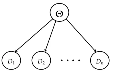
D1 D2 Dn

Θ

Figure 1.3: A Simple Bayesian network in which random variablesD1toDnare

con-ditionally independent givenΘ.

dom variable defined as the summation ofnindependent and uniformly distributed random variables.

As another example, consider a random variableXwith probability density func-tion f(x)which is positive on the interval(a,b). Similarly, letYbe a random variable with densityg(x)being positive on the interval(c,d). As [Glen et al. 2004] shows, the density function of their productV =XYis:

h(v) =



      

      

Z v/c

a g

v

x

f(x)1

x dx ifac< v<ad

Z v/c

v/d g

v

x

f(x)1

x dx ifad<v<bc

Z b

v/dg

v

x

f(x)1

x dx ifbc< v<bd

1.1.4 Piecewise likelihoods

Figure 1.3 represents a very simple Bayesian network(a graphical model that will be introduced in Chapter 2) in which, conditioned on a random variableΘ (called, pa-rameter), random variables D1 to Dn (called, data) are independent. With respect to

Bayes rule,p(Θ|D1, . . . ,Dn), the posterior distribution ofΘconditioned on observed

variablesD1to Dnis proportional to the product of the prior distribution p(Θ)times

likelihood functionsp(Di|Θ):

p(Θ|D1, . . . ,Dn)∝ p(Θ) n

∏

p(Di|Θ)

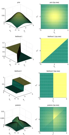
−5 0 5 −5 0 5 0 0.01 0.02 θ₁ prior

θ₂ −5−5 0 5

0 5

θ₁ prior (top view)

θ2 −5 0 5 −5 0 5 0.4 0.5 0.6 0.7 θ₁ likelihood 1

θ₂ −5−5 0 5

0 5

θ₁ likelihood 1 (top view)

θ2 −5 0 5 −5 0 50 0.5 1 θ₁ likelihood 2

θ₂ −5−5 0 5

0 5

θ₁ likelihood 2 (top view)

θ2 −5 0 5 −5 0 50 0.005 0.01 θ₁ posterior

θ₂ −5−5 0 5

0 5

θ₁ posterior (top view)

θ2

posterior∝prior×likelihood 1×likelihood 2

kx−ak< 50

kx−bk<50 kx−bk< 50

N(x,Σ1) N(x,Σ2) N(x,Σ3)

Figure 1.5: An extended algebraic decision diagram (XADD) representing the distri-bution of the predicted location of a mobile device in the example provided in Sec-tion 1.1.5. The LocaSec-tion of the device and two radio antennas are represented byx,a andb, respectively. (Solid and dotted lines represent edges to a low and high children respectively.)

1.1.5 Context-specific conditional densities

Decision diagrams and context-specific conditional probability distributions such as tree-CPDs and rule CPDs are natural structures extensively used to represent discrete models in cases where structural regularities arise in some contexts. In the case of con-tinuous models, context-specific conditional densities correspond to piecewise den-sity functions. For instance, consider the following mobile device localization model:

Example 1. The location of a mobile device is performed via multilateration of radio signals between radio towers positioned at locationsa = (a1,a2)andb = (b1,b2)as well as GPS

signals. The coverage range of each antenna tower is 50 meters. If the device position (say,

x = (x1,x2)) is within the coverage range of both antennas, the distribution of its predicted

location y is a bivariate normal distribution N(x,Σ1). If the device location is within the

range of only one antenna, the distribution of its predicted location isN(x,Σ2)(less precise)

and if it is not in the range of any antenna, the distribution follows byN(x,Σ₃)(least precise localization):

p(y|x) =



    

    

N(x,Σ1) ifkx−ak<50, kx−bk<50

N(x,Σ₂) ifkx−ak ≥50, kx−bk<50

N(x,Σ2) ifkx−ak<50, kx−bk ≥50

N(x,Σ₃) ifkx−ak ≥50, kx−bk ≥50

Develop

Time (D) Outsource Security(ModuleM) Security(ProjectA)

Module Value (V)

Figure 1.6: An influence diagram representing a situation where a company plans whether to outsource the development of a new software module or does not do so. The uncertainty nodes are Develop. speed (representing the time it take to develop the module internally),Module security(representing the quantification of the security level of the module to be developed) and Project security (representing the security level of the existing project modules). The decision node,Outsource, indicates whether to outsource the module or not. The value node,Module value, is a function of devel-opment speed and the security of the new project augmented with the module.

1.1.6 Influence diagrams

An influence diagram (ID) is a generalization of a graphical model in which along with probabilistic inference problems, decision making problems are modeled (based on maximizing expected utility criteria) [Howard and Matheson 2005].

An ID is a directed acyclic graph with three different kinds of nodes:

• random nodes, a.k.a. uncertainty nodes which are represented as ovals and are associated with probability distribution or density functions. An ID exclusively made of random nodes is a graphical model.

• decision nodeswhich are represented as rectangles and indicate the options avail-able for a decision-maker.

• An often singularvalue nodethat is represented by a diamond and is associated with a utility function upon which the decision-maker acts.

To solve for an ID is to find an optimal action policy that maximizes the expected utility associated with the value node.

ID Value nodes/utility functions can be sophisticated and in many applications piecewise. An example of an ID for which the natural modeling requires a piecewise value function is presented in Figure 1.6. This ID corresponds a situation where a software company requires adding a new module to an existing project.

The solution to this ID is to decide optimally whether to outsource the new mod-ule or develop it internally w.r.t. a utility functionuV(·)which is a function of three

• Development time (D): The amount of time it takes to develop the module in the company compared to outsourcing.

• Module security (M): Security factor associated with developing the module in-side the company as opposed to relying on the third parties.

• Project security (A): Security factor associated with the existing project code. Let utility element associated with the above factors be fD(·), fM(·) and fA(·),

respectively. The total security of a system is the minimum of the security of its com-ponents. Therefore, the utility element associated with the security of the new module added to the existing code is the minimum of the two security utility elements. As a result, it is natural to model the total utility function in a piecewise manner as below:

uV(D=d,M=m,A= a) = fD(d) +min(fS(m) + fS(a))

=

(

fD(d) + fS(m) if fS(m)≤ fS(a)

fD(d) + fS(a) if fS(m)> fS(a)

An efficient way to solve an ID is to reduce it to an ordinary graphical model [Zhang 1998]. This involves the replacement of the value node with a newly intro-duced random variable probability of which is typically proportional to the utility of the original value node plus some bias [Cooper 1988].

Therefore, an ID with piecewise utility function corresponds to a piecewise graph-ical model. Piecewise functions provide an appropriate and natural framework for ID modeling and some existing ID modeling/inference formalisms such as [Cobb and Shenoy 2004] are already based on piecewise functions.

1.1.7 Probabilistic programming

Emerging probabilistic programming languages (PPLs) try to unify general purpose programming with probabilistic modeling [Vajda 2014]. While the input values of a function in a general purpose programming languages typically consists of determin-istic values, the inputs of a PPL function may be distributions over random variables. Therefore, in a PPL function, computations take place over uncertain data and the function output is an implicitly defined distribution over the possible output values.

In PPL, conditional statements (i.e. if-statements) are intrinsically piecewise, lead-ing to piecewise output distributions.

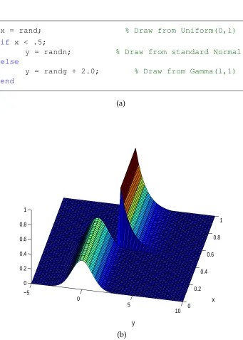
As an instance, a simple probabilistic program that includes a conditional state-ment is presented in Figure 1.7-a.3 As it can be seen in Figure 1.7-b, its corresponding joint distribution is piecewise.

The application domain examples presented in the above subsections is sufficient to illustrate the need for a general probabilistic inference algorithm that can robustly

3_{This example is taken from http://people.seas.harvard.edu/˜dduvenaud/talks/}

x = rand; % Draw from Uniform(0,1)

if x < .5;

y = randn; % Draw from standard Normal

else

y = randg + 2.0; % Draw from Gamma(1,1)

end

(a)

−5

0

5

10 0 0.2

0.4 0.6

0.8 1

0 0.2 0.4 0.6 0.8 1

x

y

(b)

handle piecewise graphical models. The aim of the current work is to move a step in the direction of designing such an inference tool.

1.2

Contributions

The focus of this thesis is on the design of probabilistic inference tools that perform well in the presence of piecewise and typically discontinuous models. As such, we propose new samplers which perform much better on piecewise models compared to their baseline counterparts. For the reasons that will be mentioned shortly, our con-tributions are based on Gibbs sampling [Casella and George 1992] and Hamiltonian MCMC [Neal 2011] methods.

1.2.1 Gibbs sampling on piecewise models.

To start with, we concentrate on the Gibbs sampling mechanism: Gibbs sampling is a powerful particle-based tool that in the context of inference on piecewise models, is arguably the first choice. The reason is that in contrast to most samplers, on such models Gibbs sampling performs well in terms of convergence to the true distribution. Nonetheless, Gibbs sampling has major drawbacks that in practice limit the do-main of its usage:

1. Gibbs sampling is typically slow since it requires several (univariate) integra-tions per sample. More precisely, per sample and for each random variable in the space of the model, Gibbs instantiates the remaining variables and computes a univariate PDF integral. This integration process can be computationally quite costly.

2. Univariate integrations required for Gibbs sampling are not always computable in closed-form.

1.2.1.1 Linear time Gibbs sampling on piecewise models

In our first contribution, we focus on piecewise polynomial density functions. Since in these models the integration can be carried out in closed-form, only the first draw-back needs to be addressed. This drawdraw-back, nonetheless, can be quite challenging on piecewise models which consist of a large number of partitions. An example of such a scenario has already been provided in Section 1.1.4 where it was shown that in a Bayesian model with piecewise likelihoods, the number of pieces in the posterior density may grow exponentially in the number of observations. As a matter of fact, this example is an instance of the following more general problem: In a graphical model with piecewise factors, the number of pieces in the joint distribution may grow exponentially in the number of factors.

model can be treated as a mixture of truncated densities. Drawing a Gibbs sample from the mixture model is equivalent to Gibbs sampling from a fixed number of par-titions in the original model. This significantly decreases the amount of computation required for Gibbs sampling. The trade-off is a slower Monte Carlomixing rate. That is, compared to the baseline Gibbs sampling, in order to converge to the true distribu-tion, more samples are required. Nonetheless, as it will be shown, in high dimensional models, the latter effect is not significant and compared to the naive Gibbs sampler implementation, in order to reach an arbitrary precision, our proposed algorithm il-lustrates an exponential to linear decrease in the total sampling time.

1.2.1.2 Fully-automated symbolic Gibbs sampling on an expressive family of piece-wise models

As an orthogonal contribution we deal with the second drawback of Gibbs sampling. We study a highly expressive family of models which are not studied in the literature so far:Piecewise fractions (of polynomials) with polynomial partitioning constraints.

Not only for a large range of such models, univariate Gibbs integrals can be com-puted in closed-form but we can also compute such integrals without instantiating the remaining variables. This immediately leads to our second contribution that is

Fully-automated symbolic Gibbs sampling.

We create a mapping from random variables to their corresponding analytical in-tegrals which are computed only once and prior to the actual sampling process rather than per sample. Consequently, multiple integrations per sample are reduced to mul-tiple function evaluations per sample which is significantly faster.

It should be pointed out that the target family of models has interesting character-istics such as being closed under a large range of (non)linear random variable transfor-mations. This opens new doors to application domains such as handling deterministic constraints among random variables.

1.2.2 Hamiltonian Monte Carlo on piecewise models

To apply the proposed Gibbs samplers on arbitrary models, they should be approx-imated by piecewise polynomials or fractional functions. This is a major drawback since such approximations may not be easy to find or the number of required parti-tions may grow exponentially with dimensionality. On the other hand, like any other class of functions, piecewise polynomial/fractional models have their own shortcom-ings. Most notably, in graphical models with huge number of factors, computation of the joint posterior requires several polynomial/fractional multiplications which can be sensitive to numerical errors. For such graphical models, the family of (piece-wise) exponential distributions is more suitable since in order to multiply distribu-tions/factors of the latter class, it is sufficient to add their logarithms.

contribu-tion, we focus on sampling from piecewise distributions without any assumption on the form of the modeling functions in any partition. Instead of Gibbs sampling we turn to Hamiltonian Monte Carlo (HMC), a particle-based inference method that has become quite popular in the recent years and has been utilized in the state-of-the-art probabilistic programming language STAN [Stan Development Team 2014].

Unlike Gibbs sampling, HMC works with the logarithm of densities and there-fore is less sensitive to numerical errors.4 HMC does not require any assumption on the class of distributions; therefore, in theory it can be used on any continuous space model. Nonetheless, on the piecewise models, its performance can be disastrously poor. A brief explanation is as follows: HMC sampling is motivated by Hamiltonian dynamics in physical systems. More precisely speaking, in HMC, the negated log-arithm of a density is assumed to be a potential energy function and to generate a sample, the trajectory of a particle is followed using the Hamiltonian dynamics. In HMC, Hamiltonian equations are approximated by methods such asleapfrog integra-tion or similar algorithms. Such methods can produce very poor simulations if the energy function is discontinuous which is typically the case with piecewise models.

Our contribution is to design a variation of HMC sampling method, calledreflective HMC(RHMC), the performance of which does not deteriorate in piecewise models. Being motivated by the behavior of Hamiltonian dynamics of physical systems such as optics, we generalize HMC and its leapfrog integration mechanism to become ap-propriate for piecewise/discontinuous models. For instance, a moving object that hits an obstacle either passes over it or bounces back. Similarly, light may reflect or refract over a refractive surface. In any case, the momentum vector in the collision point (which is a point where the potential energy is discontinuous) is modified in such a way that the system’s Hamiltonian remains unchanged.

A key point for the correctness of HMC is the volume preservation property of Hamiltonian dynamics. Due to this property, the Hamiltonian trajectories can be used to define complex mappings without requiring to perform any adjustment via a Ja-cobian factor [Neal 2011]. It is well known that this property holds even if the dy-namics are approximated via the leap frog algorithm or a similar mechanism. We prove that the volume preservation property also holds under reflection and refrac-tion mappings. This guarantees the correctness of the proposed method and as our empirical results show, it can significantly outperform the baseline HMC and be much less sensitive to the parameter tuning.

1.3

Thesis outline

In this chapter we introduced and motivated the research problem that we are inter-ested in: efficient particle-based inference in piecewise graphical models. The remain-der of the thesis is structured as follows: Chapter 2 provides the background material required to understand exact and approximate probabilistic reasoning in graphical

4_{HMC has its own problems: unlike Gibbs, it requires input parameters, and its performance can}

Probabilistic Graphical Models

This chapter contains background material regarding representation and inference on probabilistic graphical models. Probability theory is a formalism for the analysis of random phenomena. Our primary focus is on multidimensional continuous proba-bility functions p defined in the most natural way. A formal set of definitions and assumptions representing the basic probabilistic model that we are interested in, is presented in Section 2.1. The representation and inference on probabilistic graphical models are dealt with in Sections 2.2 and 2.3 respectively.

2.1

Basic Definitions and Assumptions

Outcome.The result of a single execution of a probabilistic model is called anoutcome. Sample space. The set of all possible outcomes is referred to assample space(Ω). Event.Aneventis a set of zero or more outcomes.

Probability space & measure. Aprobability spacehΩ,F,piis a tuple of asample space

Ω, a collectionF of events (to be considered) that forms aσ-algebra and aprobability measure pi.e. a function that assigns values (probabilities) to events inF. The measure

phas to satisfy the following properties: 1. p(∅) =0

2. p(Ω) =1

3. if (a countable collection of) eventsE1,E2, . . . are pairwise disjoint sets then the probability value assigned to the union of them is equal to the summation of their probabilities (countable additivityproperty).

As it is commonly done, throughout, in caseΩis countable we assumeF is the power set ofΩand if it is uncountable we letF be theBorel algebraofΩ.1

(Univariate) random variable. A (single) random variableis a measurable mapping

1_{Borel algebra is the smallestσ-algebra that makes all open sets measurable.}

fromΩto another measurable space (state space). Throughout we only consider ran-dom variables where the set of real numbers is their associated state space. That is,

X:Ω→_R

p(X=x)is a short-form for the probability of the event:

{ω∈Ω : X(ω) =x}

Probability mass function (PMF) & probability density function (PDF). In case a random variable is discrete (i.e. takes discrete realizations), probability measure is called a probability mass function (PMF) and if it is continuous, the measure is called

probability density function(PDF) or simplydensity. Throughout, when there is no am-biguity about whether the model is discrete or continuous, or if both cases are in-tended, we may refer to the probability measure simply as thedistribution.

Multivariate random variable & joint density function.Throughout, we use bold let-ters to represent vectors of elements. Amultivariate random variableX = (X1, . . . ,Xn)

is a vector of random variablesX1toXnwith the followingjoint density function:

p(X1= x1, . . . ,Xn =xn):= p{ω∈Ω : X1(ω) =x1, . . . ,Xn(ω) =xn}

We denote random variables by capital letters (e.g.Xi) and their realizations by small

letters (e.g.xi). Nevertheless, in case there is no ambiguity, we may omit the random

variables (i.e. writingp(x1,x2)instead ofp(X1 =x1,X2 =x2)). We may also omit the realizations (i.e. writing p(X)instead of p(X = x)) in case the statement holds for all realizations.

Marginal distribution. For continuous random variables the following equality al-ways holds:

p(xi) =

Z

p(x1, . . . ,xn)dx1. . . dxi−1dxi+1. . . dxn

The above integration is calledmarginalization(ofX−i i.e. all random variables except

Xi). In this context, p(xi)is referred to as themarginal distribution.

Similarly, if a marginalized random variable is discrete, its associated integration is replaced by summation over its possible values. For instance, in case all X−i are

discrete,

p(xi) =

_∑

. . .

_∑

xi−1∈VAL(Xi−1)

∑

. . .

_∑

xn∈VAL(Xn)

p(x1, . . . ,xn)

Cumulative distribution functionF(CDF).(Joint) cumulative distribution function, de-noted asF(x1, . . . ,xn)or CDF(x1, . . . ,xn), represents the probability that each random

variableXitakes on a value not greater thanxi:

Each CDF has the following properties:

1. Being monotonically non-decreasing for each of its variables 2. Being right-continuous for each of its variables

3. 0≤ F(x1,· · · ,xn)≤1

4. limx1→+∞,···,xn→+∞F(x1, . . . ,xn) =1

5. limxi→−∞F(x1, ...,xn) =0, for alli=1, . . . ,n

Clearly, the density function can be derived from the CDF as follows:

p(x1, . . . ,xn) =

∂nF(x1, . . . ,xn) ∂x₁· · ·∂x_n

Conditional probability. By definition, the conditional probability of a random vari-able or a vector of random varivari-ables (or more generally, an event) Xgiven observed

random variable(s) (resp. event)Yis,

p(X|Y):= p(X,Y)

p(Y) (2.1)

Independence.LetXandYbe a pair of random variable(s) (or more generally, events). We denoteX⊥Yand sayXandYare independent if and only if,

p(X|Y) = p(X) (2.2)

Clearly, ifX⊥YthenY⊥Xsince relations (2.1) and (2.2) imply, X⊥Y ⇒ p(X, Y) =p(X)·p(Y)

Conditional independence. A pair of random variablesXandY(or more generally two events) areconditionally independentgiven a third random variableZ(resp. event) (denoted as:X⊥Y|Z) if and only if,

p(X,Y|Z) =p(X|Z)·p(Y|Z)

Expected value. Theexpected value(orexpectation) of a (continuous) random variable

X(w.r.t. a reference distributionp) is,

E[X]:=

Z

x·p(x)dx

A similar definition exists for discrete random variables where instead of integration, summation over all possible values ofXis computed:

E[X]:=

∑

x

x

x

x

x

Figure 2.1: A Bayesian network representing the joint probability distribution over random variablesX1toX5for the example provided in subsection 2.2.1.

2.2

Representation of Graphical models

The framework of probabilistic graphical models (GMs) provides graph structured specifications of probabilistic models. Using GMs, joint distributions are represented in compact and factorized manners by means of exploiting conditional dependen-cies between random variables.2 Such dependency structures are used to design au-tomated, scalable and effective inference algorithms for the associated probabilistic models.

In this section we focus on introducing common graphical model representations while the associated inference algorithms are postponed to Section 2.3. Two main families of graphical models are:

1. directed acyclic models, known asBayesian networks(BNs), and 2. undirected models referred to asMarkov random fields(MRFs).

After introducing these two families of GMs, we present a more general framework, namelyfactor graphs, that encompasses both aforementioned families.

2.2.1 Bayesian networks (BNs)

ABayesian network also known as a probabilistic directed graphical modelis a directed acyclic graph (DAG) suitable for representation of conditional dependencies of ran-dom variables suitable. In such networks, each vertex represents a distinct ranran-dom variable (therefore, the termsvertexandrandom variablemay be used interchangeably throughout). Whenever an arrow between two vertices is missing, it means that their corresponding random variables are (conditionally) independent. For example, con-sider a probability distribution over five variablesX1toX5. The general form of such a distribution can be factorized as follows:

p(x1,x2,x3,x4,x5) =

p(x1)·p(x2|x1)·p(x3|x1,x2)·p(x4|x1,x2,x3)·p(x5|x1,x2,x3,x4)

2_{The main references of this section are [Bishop 2006; Koller and Friedman 2009; Russell and Norvig}

D1

Dn

Figure 2.2: A Bayesian network representing the Bayesian paradigm.

Nevertheless, The Bayesian network depicted in Figure 2.1 visualizes the case where

X1 andX2are independent (i.e. X1 ⊥ X2) (since no arrow links them) and givenX2,

X3 andX4are independent (i.e. X3 ⊥ X4|X2) , etc. It can be seen that in such a case, the aforementioned factorization can be simplified to,

p(x1,x2,x3,x4,x5) =p(x1)·p(x2)·p(x3|x1,x2)·p(x4|x2)·p(x5|x4)

More generally, if we letX = {X1, . . . ,Xn}be the set of all relevant random

vari-ables (i.e. the set of all vertex labels in the model) and the set of parents of a vertex

Xi ∈ X in a Bayesian network be represented by PA(Xi), that network represents a

joint distribution that factorizes into,

p(x) =

n

∏

p(xi|PA(xi)) (2.3)

Bayesian networks and conditional independence. Each Bayesian network has the following properties:

• Local Markov property: Any random variable is conditionally independent of its non-descendant vertices given it’s parent variables,

Xi ⊥X\DE(Xi)|PA(Xi)

whereDE(Xi)denotes the set of descendants ofXi (including itself).

• Each random variable is conditionally independent of all other variables in the network given itsMarkov blanketi.e. its parents, its children and all other parents of its children.

2.2.1.1 Bayesian inference / Bayesian paradigm

thatD1toDnare identically distributed and independent from each other:

Di ⊥ Dj |Θ ∀i,j6= i∈ {1, . . .n}

Figure 2.2 depicts a Bayesian network representing this paradigm whereΘ is re-garded as a hidden random variable andD1toDnas observed vertices. According to

the topology of this network,

p(Θ,D1, . . . ,Dn) =p(Θ) n

∏

p(Di|Θ)

In addition, by the definition of conditional probability,

p(Θ|D1, . . . ,Dn) =

p(Θ,D1, . . . ,Dn)

p(D1, . . . ,Dn)

∝ p(Θ,D1, . . . ,Dn)

Combining these two relations, it is clear that theposteriordistributionp(Θ|D1, . . . ,Dn)

is proportional to the product of the priordistribution p(Θ) andlikelihoodfunctions

p(D1|Θ)to p(Dn|Θ),

p(Θ|D1, . . . ,Dn)∝ p(Θ)· n

∏

p(Di|Θ) (2.4)

2.2.2 Markov random fields (MRFs)

Markov random fields (MRF) also known asundirected graphical modelsform the sec-ond major class of graphical models. In contrast to BNs, an MRF network is a graph representation where edges do not carry directional information. MRFs provide a different perspective of the independence structure among random variables and are more suitable for modeling phenomena where a directionality cannot be naturally ascribed to the interaction between random variables.

Let Gbe an undirected graph where the vertices represent a set of random vari-ablesX = {X1, . . . ,Xn}andCL(G)represent the set ofmaximal cliques3ofG. Also let

for anyC ∈ CL(G), VA(C)is the set of variables in C. With respect toG, Xforms a Markov random field if the joint distribution can be factorized overCL(G) as,

p(X) = 1

Z_C∈

∏

In the above equation,Zis a normalization constant andψ_Cis a strictly positive func-tion called a potential functionof clique C. If potential functions are represented by exponentials4,

ψ_C(VA(C)) =exp(−E(VA(C)))

3_{Amaximal cliqueof an undirected graph,G, is a subgraph of it that is a complete graph and is not a}

proper subset of any subgraph ofGwhich is a complete graph.

x

x

x

x

x

f

f

f

f

f

Figure 2.3: Afactor graphrepresenting the same distribution as the Bayesian network in Figure 2.1

Eis called anenergy function. Obviously, in case a relatively low (or high) energy is assigned to a set of variable values, a higher (resp. lower) probability is assigned to those values.

Markov random fields and conditional independence. Each MRF associated with a model with random variablesX={X1, . . .Xn}has the following properties:

• Pairwise Markov property: Any two distinct random variablesXi andXj that

are not connected by a link are conditionally independent given the rest of vari-ables:

p(xi,xj|x\{xi,xj}) =p(xi|x\{xi,xj})·p(xj|x\{xi,xj})

or more concisely:

Xi ⊥ Xj |X\{Xi,Xj}

• Local Markov property: Any variable Xi is conditionally independent of all

other variables given the set of its neighborsNE(X_i):

Xi ⊥X\(NE(Xi)∪ {Xi})|NE(Xi))

• Global Markov property: Let A and B be two distinct subsets of X (equiva-lently, two subgraphs of a MRFG) andCbe aseparating subseti.e. a subset ofG

such that any graph path containing a member of Aand a member ofBpasses through (i.e. contains a member of)C:

A⊥B|C

2.2.3 Factor graphs

Bayesian networks and Markov random fields are two subsets of a more general framework:Factor graphs.

factor-ized as:5

p(X) =

m

∏

fs(Xs) (2.6)

where as before,X={X1, . . . ,Xn}, for all 1 ≤s≤m, eachXs⊂Xand fsis a function

of them. Clearly, both factorization mechanisms of relations (2.3) and (2.5) can be seen as special cases of relation (2.6).

Factor graph structure.The factor graph of anobjective function p(·)is a data structure visualizing how variablesXand local functions{fi}mi=1factorize p(X). It is a bipartite graph withn variable-typednodes and m factor-typed nodes. Each variable node rep-resents an (observable/ hidden) variable inXand each factor node represents a local function such that the node corresponding fk is linked to the variable nodes

corre-spondingXk.

As an instance, Figure 2.3 is a factor graph representation of the distribution which is visualized by Figure 2.1. Here, factor nodes correspond to the following functions:

fa = p(x1) fb= p(x2) fc = p(x3|x1,x2)

fd = p(x4|x2) fe = p(x5|x4)

2.3

Inference in Graphical Models

The task of inference on a graphical model is to compute the posterior probability distribution of somequery variables(corresponding somehiddennodes), given a set of

evidence variables(observednodes) [Russell and Norvig 2003].

LetQ={Q1, . . . ,Qm}be the set of query variables,E= {E1, . . . ,En}be the set of

evidence variables andU={U1, . . . ,Uk}be the set of variables neither mentioned in

the query nor in the evidence. Also let(Q=q), be the short form for, (Q1 =q1, . . . ,Qm= qm)

(E=e)be the short form for,

(E1 =e1, . . . ,En=en)

and(U=u)be a short form for(U1= u1, . . . ,Uk =uk), etc.

By Bayes rule, the posterior probability of a queryQgiven an evidenceEis pro-portional to the joint distribution ofQandE. Therefore, the random variables of the Bayesian network neither inQnor inEshould be marginalized out.

5_{Instead of the product, in some contexts, factorization is performed by summation (see e.g. [Yedidia}

p(Q=q|E=e) = p((Q=q),(E=e))

p(E=e) =

Z +∞

u1=−∞. . .

Z +∞

uk=−∞

p(U=u,Q=q,E=e)du1. . . duk

Z +∞

u1=−∞. . .

Z +∞

uk=−∞ Z +∞

r1=−∞. . .

Z +∞

rm=−∞

p(U=u,Q=r,E=e)du1. . . duk dr1. . . drm

Clearly, if a marginalized variable is discrete, instead of integration, the summation over its possible values should be computed. For instance, in a network whereUand Qare discrete:

p(Q=q|E=e) = p((Q=q),(E=e))

p(E=e) =

∑

. . .

_∑

uk∈VAL(Uk)

p(U=hu1, . . . ,uki,Q=q,E=e)

∑

u1∈VAL(U1)

. . .

_∑

uk∈VAL(Uk)

∑

. . .

_∑

rm∈VAL(Qm)

p(U= hu1, . . . ,uki,Q= hr1, . . . ,rmi,E=e)

whereVAL(Vi)is the set of possible values of random variableVi.

In either case, calculations required for the computation of marginal distributions are quite expensive. As a matter of fact, the most important challenge facing prob-abilistic inference is to carry out marginalization efficiently. As such, the inference techniques that will be presented shortly, try to perform this task in an effective way.

2.3.1 Exact inference

Exact inference is possible only if the marginal distributions have closed form solu-tions. For continuous random variables, this is often not the case. As such, in this section our focus is on discrete models.

As mentioned in the previous chapter, both Bayesian networks and Markov ran-dom fields are subsets of factor graph. As a result, to cover both cases, we present the inference algorithms on the factor graphs only.

The main task of inference in factor graphs is to compute an expression of a form that is known assum-productwhen random variables are discrete:

∑

. . .

_∑

Z1φ

∏

(or more concisely∑Z∏φ∈Φφ) whereΦis a set of factors6andZ={Z1, . . . ,Zk}is the

set of variables that should be marginalized out. The following exact inference tech-niques find ways to perform such a computation with minimum repeated operations.

6_{Each factorφis a function fromVAL(X}

1)×. . .VAL(Xn) toRwherex = {Xi}in=1 is the set of all

2.3.1.1 Variable elimination (VE)

Algorithm 1:Variable elimination algorithm for factor graphs (following [Koller and Friedman 2009])

proceduresum-product-VE (

Φ/*set of factors*/,

Z/*k-tuple of variablesZ1, . . . ,Zkto be eliminated sequentially*/)

fori= 1tokdo

Φ←sum-product-eliminate-a-var(Φ,Z_i) end for

return∏φ∈Φφ

proceduresum-product-eliminate-a-var (

Φ/*set of factors*/,

Z/*a variable to be eliminated*/)

/*createΦ0, the set of all factors that involveZ: */

Φ0 ← {φ∈Φ|Z∈ SCOPE(φ)}

/*createΦ00, the set of all factors that do not involveZ: */

Φ00 ←Φ\Φ0

/*createψ, the product of the factors that involveZ: */

ψ ←∏φ∈Φ0φ

/* make a new factorτby summing outZonψ: */

τ ←∑Zψ

/*return the set of factors that do not involveZplus a factor that is made by summing outZin the factors that involve it: /*

returnΦ00∪ {τ}

The idea behind the variable elimination algorithm is the observation that the scope of each factor (i.e. the set of variables involved in that factor) is often a small subset of the total model random variables and this allows us to utilize the reverse distributive law andpush in each∑Zi to the right till it operates only on the factors that have the variableZi in their scope.

In order to calculate the sum-product∑Z∏φ∈Φφ, the VE algorithm eliminates (i.e.

marginalizes) one variableZ_i at a time. It finds the set Φ0 of factors that have Z_i in their scope, multiplies them to make a new factorψand finally, sums outZi onψ to

make a new factor that should replaceΦ0inΦ(see Algorithm 1) [Koller and Friedman 2009].

As an example consider the a set of (discrete) reference random variablesXand a set of factorsΦ, defined as follows:

where the subtitle of each factor indicates the variables mentioned in it. For instance,

SCOPE(φ_BC) ={B,C}

If the ordered list of variables that should be eliminated is Z = hA,B,Ci (so that variables are eliminated in the alphabetic order), the final factor produced by VE is:

f1(D):=

_∑

C

φ_CD

_∑

B

φ_BC

_∑

(φ_ABφ_A)

One the other hand, if the variables are eliminated in the reverse order i.e. Z0 =

hC,B,Ai, the result of VE will be:

f2(D):=

∑

A

φ_A

_∑

B

φ_AB

_∑

C

(φ_CDφ_BC)

Both f1(·)and f2(·)are clearly equivalent to the following (non-factorized) function:

f(D):=

_∑

C

∑

∑

(φ_Aφ_ABφ_BCφ_CD)

Nevertheless, either f1(·)or f2(·)can be computed much more efficiently than f(·) because intermediate factors that are created by marginalization are simpler than the original factors.

2.3.1.2 Clustering (join tree) algorithms

Clustering algorithms provide an effective way to compute posterior probabilities for each variable in the network. In this approach an algorithm calledbelief propagationis executed over a data structure calledclique tree. These concepts are defined below: Cluster tree. A cluster treeU for a set of factors Φ over a set of random variables

{X1, . . . ,Xn}is an undirected graph such that its nodes are (associated with) clusters

(a.k.a.cliques)Ciwhich correspond to subsets of random variables in the original

net-work, that is:

Ci ⊆ {X1, . . . ,Xn},

and any edge linking clustersCi andCj is associated with a set of random variables

calledsepset Si,j:

Si,j =Ci∩Cj

A cluster tree must preserve the following two properties:

1. Family preservation property: For each factorφ_k(inΦ), there should exist (at least one) clusterC_α(k) in U such that Scope[φk] ⊆ Cα(k). Otherwise stated, cluster

Cα(k)should be able to accommodate factorφk. This property guarantees thatU

allowsΦto be encoded.

2. Running intersection property: For any variable Xi, the set of nodes and edges

information about all variables without any feedback loops.

Clique tree. A clique tree (also know as join tree or junction tree) is a directed tree simply made by orienting a cluster tree. To do so, an arbitrary node in the cluster tree is designated as the root and the edges are directed toward this node.

Belief propagation (BP).BP is amessage passing7[Yedidia 2011] algorithm applied to a clique tree to carry out inference. The idea is to catch intermediate factors computed during variable elimination and pass them via messages. This algorithm consists of the following steps:

1. Assigning factors to clusters: Given a set of factorsΦ, the model is initialized with assigning eachφ_k ∈ Φto a clusterC_α(k)such that Scope[φk]⊆Cα(k)(this can be

done with respect to the family preservation property).

2. Constructing initial potentials: To each cluster (node)Ci, an initial potentialψi(Ci)

is assigned as follows:

ψ_i(Ci) =

_∏

φ_k

3. Message initialization: All messagesδ_i→j(passing from cluster nodesCitoCj) are

initialized to 1.

4. Messaging cycle: Edges are sorted/visited from the leaves to the root. Whenever an edge(i,j)is visited, firstly the potential assigned to clusterCi is updated:

ψ_i(Ci) ← ψi(Ci)×

_∏

δ_k→i,

whereNiis the set of neighboring nodes ofCi. Then, theδi→j(the message from

nodeCi to nodeCj) is updated:

δ_i→j =

_∑

Ci\Si,j

ψ_i(Ci)

Informally speaking, δ_i→j(Si,j) is generated as follows: Firstly, the product of

all incoming messages toCi (except the one received fromCj) times the initial

potential assigned toCi is computed and then the variables inCi that are not in

Si,jare summed out from it.

5. Updating the root potential:In the end, the potential associated with the root, say

Cr, is updated:

ψ_r(Cr) ← ψr(Cr)×

_∏

δ_k→r

The resulting potentials ψ_i are proportional to the joint marginal distribution of the set of variables in cliquesCi.

7_{Message passingalgorithms are a group of solutions to the optimization problem when the problem}

2.3.2 Approximate inference by sampling (Monte Carlo methods)

When the networks are large and the nodes are connected via a huge number of links, exact inference becomes intractable and computationally prohibitive. In such situa-tions, the joint distribution has to be computed by means of approximate inference techniques. On the other hand, regardless of the size and the topology of the network, if a model is continuous (or discrete/continuous hybrid) the integrations required for marginalization often do not have closed-form solution which also necessitates ap-proximate solutions.

The most general and therefore, arguably, the most important class of approximate inference techniques is known as Monte Carlo sampling methods (a.k.a.particle-based or sampling-based methods).

The idea is to take samples from a probability distribution by means of construct-ing a Markov chain that has the original distribution as its stationary distribution.

An important characteristic of Monte Carlo-based approximate inference is that these methods provideasymptotically unbiased solutionsin the sense that if the number of samples drawn from a density function is sufficiently large, the approximation error will be arbitrarily small and in the limit tends to zero.

Prior to describing sampling mechanisms,we introduce some terminology:

Particle (sample).Aparticleξdrawn from a distributionp(X=x)assigns appropriate values,

ξ(Xi)∈ VAL(Xi)

to each random variableXi ∈X. If

Y={Y1, . . . ,Yk} ⊆X

byξhYiwe denote the event{Yi =ξ(Yi)}k_i=1.

Sampling. Sampling is the practice of simulating a distribution by means of a se-quence of (pseudo)randomly generated particles (or samples) that are distributed ac-cording to that distribution. From a set of such particles,

Ξ={ξ₁, . . . ,ξ_N}

the expectation of each function f can be approximated by

ˆ

EΞ(f) =

1

N

N

∑

f(ξ_i)

More specifically, by substituting f(ξ_i)by 1I[ξ_ihYi=y]8_:

ˆ

pΞ(y) =

1

N

N

∑

1I[ξ_ihYi=y]

which is the number of particles in which Y is valuated by y divided by the total number of particles.

2.3.2.1 Inverse transform sampling

A central prerequisite for sampling from arbitrary distributions is the ability to take samples from a uniform distribution. This can be done by variouspseudorandom num-ber generation(PRNG) algorithms or by usinghardware random number generators. Since modern programming languages are equipped with this ability, PRNG algorithms are not covered by this thesis.

Being equipped with a uniform sampler, by a simple mechanism, one can generate samples for an arbitrary continuous distribution if the (inverse of) cumulative distri-bution function (CDF) of the target distridistri-bution is provided via a mechanism known as inverse transform sampling. We only consider the univariate case. Generalization to the multivariate case is also feasible and based on the idea of mappingelementary eventsto the interval[0, 1]by associating intervals to them proportional to their prob-abilities and then uniformly taking sample from the interval.

In order to draw a sample from a continuous distribution p(X)associated with CDFF(X), it suffices to uniformly sample a numberubetween 0 and 1, i.e.

u∼ U(0, 1)

and returnx=F−1(u)i.e. a valuex∈VAL(X)such thatF(x) =u.

The proof of correctness (which is a slightly modified version of the proof pre-sented in [Devroye 1986, Chap. 2]) is as follows:

Proposition 1. Let F be a continuous CDF onRwith inverse function F−1. If U is random

variable uniformly distributed over[0, 1], then the CDF of F−1(U)is F.

Proof. We should show that p(F−1_{(U)≤x) =p(X≤ x).}

p F−1(U)≤ x= p F(F−1(U))≤F(x) , sinceFis monotonic = p U≤ F(x)

= F(x) , sinceUis uniform hence pr(U≤m) =m.

Algorithm 2 illustrates a variation of the inverse transform sampling that 1. Does not require the inverse of CDF being known. (F−1is approximated.) 2. Does not require the CDF to be normalized i.e. works with any function being

proportional to the target CDF.

Algorithm 2:INVERSETRANSFORMSAMPLING(F(·))

Input: F(x), (non-normalized) cumulative distribution function of a (univariate) random variableX. (That is, a function proportional top(X≤x).)

Output:a samples drawn forXviainverse transform sampling. /* Uniformly sample a numberuin[0,F(∞)]: */

u∼ U(0,F(∞))

/* return the approximation ofF−1(u): */ ReturnINVERSE(F,u, 0,F(∞))

// ApproximatesF−1(u) =inf{x : F(x) =u,a≤u≤ b}via binary search. procedureINVERSE(

F(·)/*a univariate monotone function*/,

u/*a value for which the inverse function has to be computed*/,

a,b/*associated lower and upper bounds*/)

l1 ←a;l2←b whiletruedo

∆= F(l1+l2

2 )−u

/*is a constant indicating the maximum acceptable approximation error. */ if|∆|<then return l1+₂l2

if∆>0then l2 ← l1+₂l2 elsel1← l1+₂l2 end while

The second property is due to the fact that if a CDF is not normalized it converges to the normalization constant and therefore, in practice the latter constant can be ap-proximated by evaluating the (non-normalized) CDF function for a large value.

Clearly, in case the support of the target distribution is finite, that is, the distribu-tion is surrounded by a 0-probability space, the aforemendistribu-tioned normalizadistribu-tion con-stant can be computed precisely: it is sufficient to evaluate the CDF for a value more than the upper bound of the support.

2.3.2.2 Forward sampling

If the task of sampling from a Bayesian network is to estimate marginal probabilities without being conditioned on particular observations, that is, if we intend to draw a sample from a prior distribution, the task can be accomplished in a fairly easy manner: It is sufficient to sample parent nodes prior to their children.

X Y

Z For instance, consider a simple BN over random variables

X, Y andZ where no vertex is observed and Z is condition-ally dependent on the other variables (as depicted in the right hand side). In this example, variable sampling order should either be hX,Y,Zior hY,X,Zi. This process is calledforward

sam-ple value to a vertex, forward sampling is performed on its associated distribution conditioned on the sample values already assigned to its parent nodes (See Algorithm 3).

Algorithm 3:A simple sampling on the prior distributions in a Bayesian network procedureFORWARDSAMPLING(

B/*a Bayesian network overX={X1, . . . ,Xn}where indices indicate a

topological ordering*/ )

Letξbe a particle vector that should be returned. fori= 1tondo

/* SampleXi conditioned on the samples already taken from its parents:*/ ξ(Xi)∼ p(Xi|ξhPA(Xi)i)

end for returnξ

The rest of this subsection deals with sampling from conditional distributions (e.g.

p(Y = y|E = e)). To be more specific, consider the problem of sampling from a Bayesian network with observed nodesE = {E1, . . . ,Ek}. In this case, the generated

samples should comply with the observation. Forward sampling cannot be directly used to sample these nodes and their parents/ancestors (although the particle values of the remaining nodes can still be generated by forward sampling as before). As a specific form of rejection sampling (that will be outlined in Section 2.3.2.3), a simple solution is to sample the prior distribution and discard the particles that do not com-ply with the observation. This technique can only be applied to discrete distributions and even in that case, if the probability of the evidence is low, the rate of discarded samples can be arbitrary large.

Therefore, sampling from posterior distributions (and in particular, continuous space posteriors) is a major challenge and in the remaining part of this subsection we deal with the relevant solutions proposed in the literature.

Before presenting such techniques, it should be pointed out that in contrast with priors distributions that often have simple forms (e.g. are uniform of normal) the posterior distributions can in particular be complicated functions e.g. may be multi-modal, disconnected and piecewise.

2.3.2.3 Rejection sampling

Rejection sampling(a.k.a. acceptance-rejectionalgorithm) is a basic Monte Carlo based sampling method.