2 3 4 5 6 7 8 9
Draft version June 27, 2018
Typeset using LATEXmanuscriptstyle in AASTeX62
Suppression of Dielectronic Recombination Due to Finite Density Effects II: Analytical Refinement
and Application to Density Dependent Ionization Balances and AGN Broad Line Emission
D. Nikoli´c,1 T. W. Gorczyca,1 K. T. Korista,1 M. Chatzikos,2 G. J. Ferland,2 F. Guzm´an,2 10
P A. M. van Hoof,3 R. J. R. Williams,4 and N. R. Badnell5 11
1Western Michigan University, Kalamazoo, MI, USA
12
2University of Kentucky, Lexington, KY, USA
13
3Royal Observatory of Belgium, Ringlaan 3, 1180 Brussels, Belgium
14
4AWE plc, Aldermaston, Reading RG7 4PR, UK
15
Corresponding author: T. W. Gorczyca
Nikoli´c et al.
5University of Strathclyde, Glasgow, UK
16
(Received; Revised; Accepted; )-17
ABSTRACT
18
We present improved fits to our treatment of suppression of dielectronic recombination
19
at intermediate densities. At low densities, most recombined excited states eventually
20
decay to the ground state, and therefore the total dielectronic recombination rate to
21
all levels is preserved. At intermediate densities, on the other hand, collisions can
22
lead to ionization of higher-lying excited states, thereby suppressing the dielectronic
23
recombination rate. The improved suppression factors presented here, although highly
24
approximate, allows summed recombination rate coefficients to be used to intermediate
25
densities. There have been several technical improvements to our previously presented
26
fits. For H- through B-like ions the activation log densities have been adjusted to better
27
reproduce existing data. For B-, C-, Al-, Si-like ions secondary autoionization is now
28
included. The treatment of density discontinuity in electron excitations out of ground
29
state H-, He-, and Ne-like ions has been improved. These refined dielectronic
recombi-30
nation suppression factors are used in the most recent version of plasma simulation code
31
Cloudy. We show how the ionization and emission spectrum changes when this physics
32
is included. Although these suppression factors improve the treatment of
intermedi-33
ate densities, they are highly approximate and are not a substitution for a complete
34
collisional radiative model of the ionization balance.
35
Keywords: atomic data, atomic processes, line: formation, plasmas, ISM: atoms,
36
ISM: abundances, galaxies: nuclei
37
1. INTRODUCTION
38
DR is an important process determining the ionization balance in cosmic plasmas. To this end, a
39
large effort has been devoted to computing a reliable database for total and partial DR rate coefficients
Suppression of Dielectronic Recombination II
(see Badnell et al. 2003, and the 14 subsequent papers in that series, as referenced by the latest one,
41
Kaur et al. (2017)). These data are necessary input to plasma simulation codes such as Cloudy
42
(Ferland et al. 2017). However, all of that data has been computed assuming a zero-density plasma
43
environment, reducing the total DR problem to a more tractable atomic physics problem consisting
44
of a single incoming electron colliding with a single atomic ion and recombining to an ionization state
45
one lower in charge, with the emission of one photon (and any additional, cascading photons).
46
It has long been recognized (Burgess & Summers 1969) that in a plasma of non-negligible density,
47
such as in the broad emission-line regions of Active Galactic Nuclei, with densities ne ∼1010 cm−3,
48
additional, secondary plasma electrons enter into the problem and may affect the total recombination
49
rate via intermediate electron-impact ionization of captured, doubly-excited resonance states,
deplet-50
ing the radiative rate and thereby the final recombination probability. Treating this more complex
51
problem requires, in addition to accurate, zero-density atomic data, a generalized collisional
radia-52
tive (GCR) model approach (Summers & Hooper 1983) to account for all possible recombination and
53
ionization pathways.
54
To date, there has been limited GCR modeling carried out, and we have relied on the
pioneer-55
ing work of Burgess & Summers (1969), and the extensive, detailed calculations for the
density,-56
temperature-, and elemental-dependent, effective recombination rate coefficient of Summers (1974
57
& 1979), as a guide for quantifying the suppression of DR due to finite-density effects. This was
58
the approach adopted by us in a previous publication Nikoli´c et al. (2013), hereafter referred to as
59
Paper I.
60
After several model applications of this algorithm, it was found in certain situations (see for example
61
Young (2018)), that the original formulation was susceptible on finer grids to numerical difficulties
62
arising from a discontinuity in temperature of the effective DR rate coefficient. This problem affects
63
the first five isoelectronic sequences: H- through B-like.
64
The present paper serves three purposes. First, a minor “tweak” to our previous formulation is
65
introduced to circumvent the earlier discontinuity in temperature of the suppression factor. Second,
66
to provide an alternative suppression factor for four sequences, following Summers (1974 & 1979),
Nikoli´c et al.
depending on the source of (physics included in) the zero-density DR rate coefficients it is to be
68
applied to. Third, representative finite-density plasma simulations are carried out using the new,
69
modified Cloudy version to assess the effect of finite densities, via the consequent DR suppression,
70
in an actual plasma environment.
71
2. GENERALIZED DENSITY SUPPRESSION MODEL
72
The present approach for treating DR suppression follows closely the original formulation ofNikoli´c
73
et al.(2013), with only minor refinement in the final algorithm, but for completeness and to avoid any
74
confusion, the entire formulation is repeated below, with the important modification highlighted. In
75
general, theeffective DR rate coefficient αeffDR(ne, T, q, N), as a function of electron density ne(cm−3)
76
and temperatureT (K), ionic charge stateq, and isoelectronic sequence (labeled byN) is suppressed
77
from the zero-density value αDR(T) (cm3s−1) by a dimensionless suppression factor SN(ne, T;q),
78
αeffDR(ne, T, q, N)≡SN(ne, T;q)αDR(T) ; (1)
for simplicity, we use the dimensionless log density parameter x= log10ne.
79
The functional form of SN(n
e, T, q) is taken to be a pseudo-Voigt profile
SN(x, T;q) =
1 x≤xa(T;q, N)
e−(
x−xa(T;q,N)
w/√ln 2 ) 2
x≥xa(T;q, N)
, (2)
of widthw= 5.64586 and an activation log densityxa(T;q, N) that is represented by the complicated
80
expression
81
xa(T;q, N) =x0a+log10
"
q q0(q, N)
7
T T0(q, N)
1/2#
. (3)
A fit of the suppression factors ofSummers(1974 & 1979) for all ions yielded a global (log) activation
82
density x0a = 10.1821 and more complicated expressions for the zero-point temperature T0(K) and
83
charge state q0. These were found to depend on both the ionic charge state q and the isoelectronic
84
sequence N viz.
85
Suppression of Dielectronic Recombination II
and
86
q0(q, N) = (1−
p
2/3q)A(N)/√q , (5)
where
87
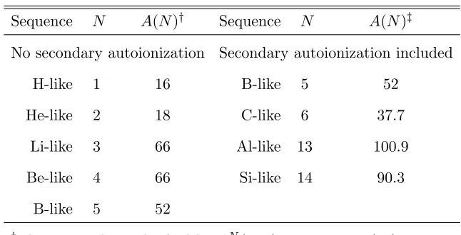
A(N) = 12 + 10N1+
10N1−2N2
N1−N2
(N −N1) (6)
depends on the isoelectronic sequence in the periodic table according to the specification of the
88
parameters
89
(N1, N2) =
(3,10) N ∈2ndrow (37,54) N ∈5throw
(11,18)N ∈3rdrow (55,86) N ∈6throw
(19,36)N ∈4throw (87,118)N ∈7throw
. (7)
If the zero-density DR dataαDR(T) in Eq. (1) neglects the secondary autoionization (Blaha 1972), this
90
parametrization is sufficient for all isoelectronic sequencesN ≥6. However, the given parametrization
91
was not flexible enough to provide an adequate fit to the Summers (1974 & 1979) data for the lower
92
isoelectronic sequences N ≤ 5. Instead, we explicitly list the optimal values for A(N), for lower
93
ionization stages, in Table 1.
94
Even with this formulation, an additional modification was necessary at electron temperatures
95
and/or ionic charges for which the q-scaled temperature θ ≡ T /q2 was very low (θ ≤ 2.5×10⁴ K,
96
which is now a slightly different formulation than that used previously.
97
In Paper I Nikoli´c et al. (2013), we modified the factorA(N) for low temperatures as follows:
98
Amod,old(N ≤5) =
A(N) , θ >2.5×10⁴ K
2×A(N) , θ≤2.5×10⁴ K
. (8)
Using this algorithm, the discontinuity in the modification factor, from unity to a factor of two at
99
θ = T /q2 = 2.5×10⁴ K, was found to cause numerical difficulties, for certain density-dependent
100
modeling applications, using the previous Cloudy release following Paper I. In order to avoid any
101
such algorithmic difficulties in the future, and also to allow for an improved fit of the available
Nikoli´c et al.
suppression factor data of Summers (1974 & 1979) by a generalized suppression formulation, we
103
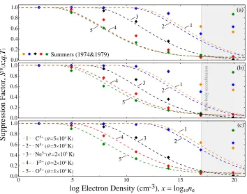
update the additional low-temperature modification factor via a continuous function:
104
Amod(N) =
ψN(q, T)×A(N), N ≤5
ψN
sec(q, T)×A(N), N = 5,6,13,14
. (9)
Here the additional dimensionless functions
105
ψN(q, T) = 2× 1 +π3×e
−(log10√T−π1 2π2 )
2
+π6×e
−(log10√T−π4 2π5 )
2
1 + e−
√
25000q2/T (10)
πi=π (1) i +π
(2) i ×q
π(3)i ×e−q/πi(4) i= 1. . .6,
106
ψsecN (q, T) = 1 +γ3×e
−(log10√T−γ1 2γ2 )
2
+γ6×e
−(log10√T−γ4 2γ5 )
2
(11)
γi=γ (1) i +γ
(2) i ×q
γi(3) ×e−q/γi(4) i= 1. . .6,
are continuous at all temperatures and ensure the same asymptotic behavior as determined before,
107
Amod(N)θ−→→∞A(N) (12)
−→
θ→0 2×A(N), (13)
and the additional flexibility introduced allows for an improved fit to the Summers (1974 & 1979)
108
data; the adjustment coefficientsπi(j) andγi(j) are given in Table2and theψN(q, T) for iso-electronic
109
sequences considered here are illustrated in Fig. 4 of AppendixA.
110
If the main concern is to remove the temperature discontinuity, while keeping the overall agreement
111
with Summers (1974 & 1979) data to better than 25%, then we suggest using the “simplified” part
112
of Table2. However, for the overall agreement withSummers(1974 & 1979) data of 14% and better,
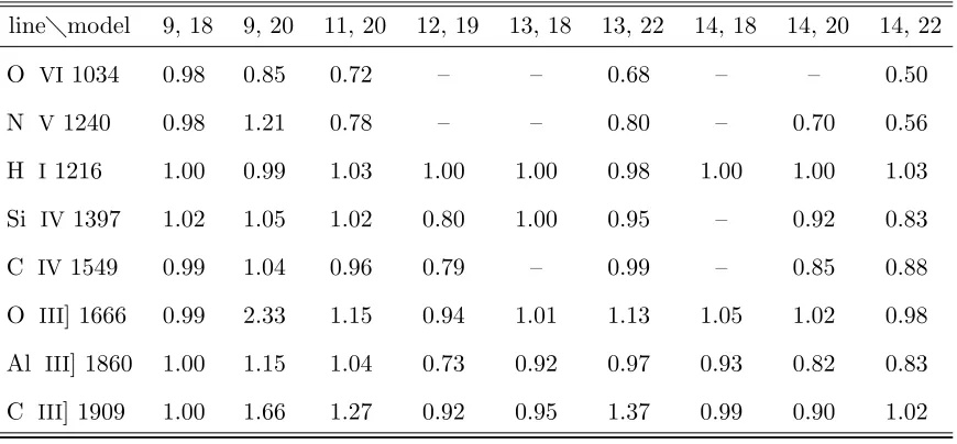
113
the use of “detailed” part of Table 2 is recommended for lowest five isoelectronic sequences. For the
114
B-, C-, Al-, and Si-like sequences effects of secondary autoionization cannot be neglected. If the
zero-115
density DR data αDR(T) in Eq. (1) for these isoelectronic sequences already accounts for secondary
116
autoionization effects, then the “secondary autoionization” part of Table 2 should be used. Note
Suppression of Dielectronic Recombination II
Table 1. ModifiedA(N) coefficients from Eq. (6).
Sequence N A(N)† Sequence N A(N)‡
No secondary autoionization Secondary autoionization included
H-like 1 16 B-like 5 52
He-like 2 18 C-like 6 37.7
Li-like 3 66 Al-like 13 100.9
Be-like 4 66 Si-like 14 90.3
B-like 5 52
† these must be multiplied byψN(q, T) given in Eq. (10)
‡ these must be multiplied byψN
sec(q, T) given in Eq. (11)
that Table 2 contains two sets of adjustment coefficients for B-like ions, depending on whether the
118
zero-density DR dataαDR(T) in Eq. (1) already contains corrections due to secondary autoionization
119
or not. The results of Paper I should be used for all other isoelectronic sequences, including C-,
120
Al- and Si-like if being applied to zero-density DR rate coefficients which do not include secondary
121
autoionization. In the 2017 release of Cloudy (Ferland et al. 2017) the zero-density DR data for
B-122
like ions is modified using the “secondary autoionization” part of Table2in accordance with modern
123
DR data of Badnell et al. (2003)1 which includes the effect. For details regarding the variation of
124
accuracy with respect to approximations used over a wide range of temperatures and isoelectronic
125
sequences see Fig. 5 of AppendixB.
126
To illustrate how much better the present algorithm reproduces the Summers (1974 & 1979)
sup-127
pression factor, we show a comparison of old and new results in Fig.1for several representative ions,
128
sequences, and temperatures as a function of electron density.
129
For even lower temperatures, we add a final modification to ensure that, at plasma energies kT
130
much less than the excitation energies, N(q), for which the intermediate resonance states are not
131
Nikoli´c et al.
Table 2. Adjustment coefficients πi(j) from Eq. (10) andγi(j) from Eq. (11).
adjustment factor: “detailed”ψN(q, T) “simplified”ψ “secondary autoionization”ψN sec(q, T)
Sequence N πi π(1)i π (2)
i π
(3)
i π
(4)
i π
(1) i π
(2) i π
(3) i π
(4)
i Sequence N γi γ(1)i γ (2)
i γ
(3)
i γ
(4) i
H-like 1 π1 4.7902 0.32456 0.97838 24.78084 0 0 0 ∞ C-like 6 γ1 5.90184 -1.2997 1.32018 2.10442
π2 -0.0327 0.13265 0.29226 ∞ ∞ 0 0 ∞ γ2 0.12606 0.009 8.33887 0.44742
π3 -0.66855 0.28711 0.29083 6.65275 0 0 0 ∞ γ3 -0.28222 0.018 2.50307 3.83303
π4 6.23776 0.11389 1.24036 25.79559 0 0 0 ∞ γ4 6.96615 -0.41775 2.75045 1.32394
π5 0.33302 0.00654 5.67945 0.92602 ∞ 0 0 ∞ γ5 0.55843 0.45 0.0 2.06664
π6 -0.75788 1.75669 -0.63105 184.82361 0 0 0 ∞ γ6 -0.17208 -0.17353 0.0 2.57406 He-like 2 π1 4.82857 0.3 1.04558 19.6508 0 0 0 ∞ Al-like 13 γ1 6.59628 -3.03115 0.0 10.519821
π2 -0.50889 0.6 0.17187 47.19496 ∞ 0 0 ∞ γ2 1.20824 -0.85509 0.21258 25.56
π3 -1.03044 0.35 0.3586 39.4083 0 0 0 ∞ γ3 -0.34292 -0.06013 4.09344 0.90604
π4 6.14046 0.15 1.46561 10.17565 0 0 0 ∞ γ4 7.92025 -3.38912 0.0 10.02741
π5 0.08316 0.08 1.37478 8.54111 ∞ 0 0 ∞ γ5 0.06976 0.6453 0.24827 20.94907
π6 -0.19804 0.4 0.74012 2.54024 0 0 0 ∞ γ6 -0.34108 -0.17353 0.0 6.0384 Li-like 3 π1 4.55441 0.08 1.11864 ∞ 0 0 0 ∞ Si-like 14 γ1 5.54172 -1.54639 0.01056 3.24604
π2 0.3 2.0 -2.0 67.36368 ∞ 0 0 ∞ γ2 0.39649 0.8 3.19571 0.642068
π3 -0.4 0.38 1.62248 2.78841 0 0 0 ∞ γ3 -0.35475 -0.08912 3.55401 0.73491
π4 4.00192 0.58 0.93519 21.28094 0 0 0 ∞ γ4 6.88765 -1.93088 0.23469 3.23495
π5 0.00198 0.32 0.84436 9.73494 ∞ 0 0 ∞ γ5 0.58577 -0.31007 3.30137 0.83096
π6 0.55031 -0.32251 0.75493 19.89169 0 0 0 ∞ γ6 -0.14762 -0.16941 0.0 18.53007 Be-like 4 π1 2.79861 1.0 0.82983 18.05422 0 0 0 ∞
π2 -0.01897 0.05 1.34569 10.82096 ∞ 0 0 ∞
π3 -0.56934 0.68 0.78839 2.77582 0 0 0 ∞
π4 4.07101 1.0 0.7175 25.89966 0 0 0 ∞
π5 0.44352 0.05 3.54877 0.94416 ∞ 0 0 ∞
π6 -0.57838 0.68 0.08484 6.70076 0 0 0 ∞
B-like 5 π1 6.75706 -3.77435 0.0 4.59785 0 0 0 ∞ B-like 5 γ1 6.91078 -1.6385 2.18197 1.45091
π2 0.0 0.08 1.34923 7.36394 ∞ 0 0 ∞ γ2 0.4959 -0.08348 1.24745 8.55397
π3 -0.63 0.06 2.65736 2.11946 0 0 0 ∞ γ3 -0.27525 0.132 1.15443 3.79949
π4 7.74115 -4.82142 0.0 4.04344 0 0 0 ∞ γ4 7.45975 -2.6722 1.7423 1.19649
π5 0.26595 0.09 1.29301 6.81342 ∞ 0 0 ∞ γ5 0.51285 -0.60987 5.15431 0.49095
π6 -0.39209 0.07 2.27233 1.9958 0 0 0 ∞ γ6 -0.24818 0.125 0.59971 8.34052
suppressed (see Paper I), the suppression is “turned off”:
132
SN(x, T;q) = 1−
1−SN(x, T;q)×exp
−N(q)
10kT
. (14)
When compared to the Paper I methodology for H-, He-, and Ne-like ions, in the present study we
133
“turn off” the suppression for these ions in continuous fashion with respect to the global activation log
134
densityx0
a, see Table5of AppendixC. We also update the excitation energy 14(2) forS2+ following
135
the results of Badnell et al. (2015). The excitation energies for other isoelectronic sequences remain
Suppression of Dielectronic Recombination II
0 . 0 0 . 2 0 . 4 0 . 6 0 . 8 1 . 0
1
2
3
4
5
( a )
l o g E l e c t r o n D e n s i t y ( c m - 3 ) , x = l o g 1 0n e
th re e-b o d y r ec o m b in at io n
S u m m e r s ( 1 9 7 4 & 1 9 7 9 )
C 5 + (q= 5 ×1 0 4 K )
N 5 + (q= 5 ×1 0 4 K )
N e5 + (q= 2 ×1 0 5 K )
O 5 + (q= 1 ×1 0 4 K )
F 5 + (q= 2 ×1 0 4 K )
0 . 0 0 . 2 0 . 4 0 . 6 0 . 8 1 . 0
5
4 3
2
1
( b )
0 5 1 0 1 5 2 0
0 . 0 0 . 2 0 . 4 0 . 6 0 . 8 1 . 0
5 4 3 2 1 2 5 4 3 2 1
( c )
S u p p re ss io n F ac to r, S
N(x
;
q
,T
[image:9.612.133.487.58.337.2])
Figure 1. Computed suppression factors for representative situations (ions, sequences, temperatures, and
densities) as compared to the GCR results of Summers (1974 & 1979). Results correspond to cases when
activation log densityxa(T;q, N) is estimated using the earlier formulation of Paper I (a), the “simplified”
ψ (b), or the “detailed”ψN(q, T) (c) adjustment factors given in Eq. (10) and Table 2.
the same as in Paper I, parameterized by the expression
137
N(q) = 5 X j=0 pN,j q 10 j . (15)
As in Paper I, these parameters are optimized using the available NIST excitation energies (Ralchenko
138
et al. 2011) and are listed in Table 5 of AppendixC.
139
3. IONIZATION AND EMISSION PREDICTIONS
140
The density dependence of the ionization rate coefficient at most astrophysical densities is negligible
141
compared to that of the (dielectronic) recombination one - see e.g. Sec. 3.2, p.5 ofSummers (1974 &
142
1979). This is a reasonable approximation since the initial state population for ionization is almost
143
exclusively in the ground (and perhaps metastables), which have little density dependence, compared
144
to excited states. In contrast, density dependence in recombination arises via the final state, and in
Nikoli´c et al.
DR these are highly-excited. The effective ”density dependent” ionization rate coefficients can be
146
downloaded from Open ADAS (Summers 2004) in ADF11 data format at two degrees of refinement:
147
(i) ‘unresolved’, in which ions are assumed to be in the ground state only, and (ii)
‘metastable-148
resolved’, in which both ground and metastable states of ions may be dominant. Section D of
149
Appendix presents the ionization balance for the lightest thirty elements for the photoionization and
150
collisional ionization cases.
151
3.1. The equivalent two-level approximation
152
Several approaches can be taken in computing the ionization distribution of the elements. In the
153
equivalent two-level approximation, which applies at low densities, recombinations to excited states
154
will eventually decay to the ground state. Only ionizations from ground need to be considered since
155
at low densities this is where nearly all of the population lies. This approximation holds for the
156
interstellar medium (ISM) and is described in texts such as (Osterbrock & Ferland 2006, hereafter
157
AGN3), and in Section 3.2 of (Ferland et al. 2017, hereafter C17). In this approximation summed
158
recombination coefficients, such as those given at http://amdpp.phys.strath.ac.uk/tamoc/DATA,
159
can be used. At high densities, the gas comes into LTE and the ionization is given by the
Saha-160
Boltzmann equation. This limit is reached in the lower parts of many stellar atmospheres and
161
accretion disks (Hubeny & Mihalas 2014). The intermediate density case is the most difficult since
162
neither limit applies and collisional processes affecting the highly-excited Rydberg levels must be
163
taken into account. In this case a “collisional radiative model” (CRM) must be done. Such models
164
are discussed in Ralchenko(2016) and Section 3.1 of C17. Section 3 of C17 used Cloudy’s full CRM
165
treatment of one and two electron systems to make estimates of the range over which the two-level
166
and LTE approximations hold. The ranges are significantly different for collisionally and photoionized
167
environments. CRM effects are important at much lower densities in the collisional case due to the
168
dominance of near-threshold collisional ionization, which also affect the Rydberg level populations.
169
In the photoionized case, the gas kinetic temperature is much lower than the ionization potentials
170
so collisional ionization is much less important. The range over which the two-level approximation
Suppression of Dielectronic Recombination II
works is also very strongly density dependent. The two-level approximation works at much higher
172
densities for higher charges q due to the well-know q−7 scaling of collisional effects, described by
173
Bates et al. (1962) and Burgess & Summers(1969). This paper develops corrections to the summed
174
recombination coefficients to improve the behavior of the two-level approximation at intermediate
175
densities. The results of this paper are included in the C17.01 update to Cloudy and we use that
176
version in the calculations presented here.
177
3.2. The case of Oxygen
178
We first focus on oxygen since it is the third most common element, has high quality DR rates,
179
and produces strong emission lines from the IR to the X-ray so has great astronomical importance.
180
Figure 2 shows the suppression factors for the first seven ionization stages of oxygen. These were
181
computed for a gas kinetic temperature of 104.5 K and various electron densities, indicated along the
182
independent-axis. This low temperature is characteristic of photoionized plasmas with a moderate
183
level of ionization and is chosen to illustrate the physics.
184 185
The density and charge dependencies reflect the decays of the highly excited levels. Suppression is
186
negligible for densities below ∼104 cm−3. For very low densities, the collisional rate is much slower
187
than the radiative decay rates so electrons captured into Rydberg levels will undergo a stabilizing
188
radiative decay and the ion recombines. The detailed density dependence is different for different
189
ions because the electron configuration affects the detailed stabilization channels, but the tendency
190
is for the importance of suppression to decrease with increasing ionization, a tendency also shown for
191
the one and two electron species in Section 3 of C17. The radiative decay rates, which stabilize the
192
recombined ion, have a rapid charge dependence,∼q4, while the collisional ionization rate coefficients
193
decrease. So, for higher charge q higher densities are needed to obtain the same suppression effect,
194
according to the ∼ q−7 effect discussed by Bates et al. (1962) and Burgess & Summers (1969).
195
The remainder of this section develops collisional- and photoionized models with and without this
196
suppression to study its effects on spectroscopic models. We note that Summers (1974 & 1979) did
197
not provide any finite-density data for the recombination of singly-charged ions to form neutrals.
Nikoli´c et al.
0
5
1 0
1 5
0 . 0
0 . 2
0 . 4
0 . 6
0 . 8
1 . 0
O
7 +O
5 +O
4 +O
6 +O
3 +S
N
(
x
;
q
,
T
)
x
= l o g
n
eN = 7 ( N - l i k e )
N = 6 ( C - l i k e )
N = 5 ( B - l i k e )
N = 4 ( B e - l i k e )
N = 3 ( L i - l i k e )
N = 2 ( H e - l i k e )
N = 1 ( H - l i k e )
l o g
T
= 4 . 5
O
2 + [image:12.612.132.487.56.338.2]O
1 +Figure 2. Suppression of oxygen DR for various ions and a temperature of 104.5 K. The legend indicates
the isoelectronic sequence of the recombining species, with O1+ indicating recombination forming O I or O0.
The logarithm of electron density is indicated along the independent-axis.
Consequently, results for neutrals should be treated with extreme caution since they follow from
199
extrapolation of doubly- to singly-charged data.
200
3.3. Ionization calculations for the lightest thirty elements
201
We consider two classes of models: the first are in electron collisional ionization equilibrium, while
202
the second is for a photoionized gas. We note that a significant amount of C, O, Si, and S form
203
molecules in the lowest temperature and electron density collisional model. Although physically
204
correct, this introduces a distraction from our main point, the density-dependent effect of DR
sup-205
pression upon the ionization. The chemistry network was disabled for the calculations presented
206
here, which has the added benefit of decoupling the results from uncertainties in the chemical rates
207
and the completeness of the chemical database. We concentrate now on oxygen and show results in
208
Figure3.
Suppression of Dielectronic Recombination II
0.01 0.10 1.00
4.0 4.5 5.0 5.5 6.0 6.5 7.0 7.5 8.0 8.5 9.0 0.1
1
10 oxygen
log Electron Temperature (K)
Dense / Vacuum
Frac. Abund.
0 . 0 1 0 . 1 0 1 . 0 0
F
ra
c.
A
b
u
n
d
.
D
en
se
/
V
ac
u
u
m
l o g U
o x y g e n
- 4 . 0 - 3 . 5 - 3 . 0 - 2 . 5 - 2 . 0 - 1 . 5 - 1 . 0 - 0 . 5 0 . 0 0 . 5 1 . 0 1 . 5 2 . 0 2 . 5 3 . 0 3 . 5 4 . 0 0 . 1
1
[image:13.612.129.483.58.588.2]1 0
Figure 3. Ionization results for oxygen for the two cases. Section Dof Appendix shows similar results for
the lightest thirty elements. The upper pair of panels is for a collisionally ionized gas and the independent
axis is the gas temperature. The lower pair of panels is for photoionization and the ionization parameter
is the independent axis. In each, the upper sub-panel shows the ionization at densities of 1 cm−3 (vacuum,
Nikoli´c et al.
In the electron collisional case, ionizing photons can be neglected and only impact ionization by
211
thermal electrons is important. Ionization by other particles such as protons and helium nuclei are
212
included but are generally negligible. As shown in the discussion around equation Eq. 4 of C17, the
213
ionization fraction has no direct density dependence if the collisional ionization and recombination
214
rate coefficients do not depend on density. The ionization fraction depends only on the temperature
215
due to the exponential dependence of the Boltzmann factor in the collisional ionization rate coefficient
216
and the slower temperature dependencies of the recombination rate coefficients. Higher ionization
217
is produced by higher temperatures, the free parameter in this case. The temperature is varied
218
over a very wide range so that the charge state of most elements ranges from fully atomic at low
219
temperatures to bare nuclei at high values.
220
We also consider photoionized clouds. Here the radiation field is the dominant source of
ioniza-tion. The photoionization rate has no temperature dependence so the recombination rate coefficients
introduce the only direct temperature dependence. That temperature is determined by the balance
between heating and cooling processes, as discussed in Chapter 3 of AGN3. Increases in the
ioniza-tion are produced by either a brighter radiaioniza-tion field, which increases the photoionizaioniza-tion rate, or by
a smaller electron density, which decreases the recombination rate. The ionization parameter U, the
dimensionless ratio of photon to hydrogen densities, (AGN3, Eq. 14.7), is defined as
U ≡ Q(H)
4πr2n(H)c ≡
Φ(H)
n(H)c , (16)
where Q(H) is the total number of ionizing photons, r the separation between the radiation source
221
and the cloud, and Φ(H) is the flux of hydrogen-ionizing photons, n(H) is the number density of
222
hydrogen, and c is the speed of light. This parameter plays the same role as the temperature in the
223
collisional case. We varyU over a broad range to change the ionization from atomic to fully ionized.
224
The gas is irradiated by a continuum with fν ∝ν−1 between 30 meV and 100 MeV.
225
In photoionization equilibrium, the gas temperature depends on the ionization parameter in a
226
complex way but generally tends to increase withU and, at constant U, increase with density due to
227
suppression of collisional cooling at high densities. These temperature changes would obfuscate the
Suppression of Dielectronic Recombination II
central point of this paper, the density-dependent suppression, since we wish to compare models with
229
different densities which will have different temperatures. To remove this confusion, we artificially
230
set the gas kinetic temperature to an intermediate value, T = 104.5 K, for all U and both densities.
231
A density of ne = 1 cm−3 is used to represent the vacuum case. As shown in Figure 2, DR is not
232
suppressed at such low densities. A density ofne= 1010 cm−3 represents an interesting intermediate
233
density. Figure 2shows that the DR is moderately suppressed at this density. The density is typical
234
of the broad emission-line regions of Active Galactic Nuclei (Korista et al. 1997) and is a
low-to-235
intermediate density in terms of the CRM. This density is low enough that the CRM effects are
236
significant but not dominant, so a modified two-level approximation should apply.
237
Suppression of the recombination coefficients will cause the ionization to increase in the two-level
238
limit. A corrected two-level approximation might then reproduce the intermediate-density rise in the
239
ionization shown in Figs 10 & 11 of C17. For these densities, the CRM effects are not yet large and the
240
two-level approximation, with modified recombination coefficients, is a reasonable approximation. At
241
very high densities, where CRM effects are severe, the gas ionization goes over to the Saha-Boltzmann
242
limit and decreases as density increases. It would be unrealistic to hope that simple corrections to
243
the two-level approximation could recover this limit.
244
Figure 3 and Figures A and B of Appendix D show results. The upper panel shows ionization
245
fractions, the dimensionless ration(ion)/n(element). The series of peaks corresponds to successively
246
higher stages of ionization reaching an abundance peak at a particular temperature or ionization
247
parameter. In the electron collisional case, the temperature of this peak is determined mainly by the
248
ionization potential, the details of the collisional ionization and recombination rate coefficients, and
249
the density suppression of the latter. In the photoionization case, the peak is sensitive to both the
250
ionization parameter and the shape of the incident radiation field, in addition to the photoionization
251
cross section and recombination rate coefficients. The lower panel shows the ratio of the ionization
252
fractions for the two densities to make the changes in the ionization easier to see. Predictions change
253
by approximately a factor of two for O, although other elements can have an order of magnitude
254
change, as Figures A and B of Appendix D show. The changes are largest for intermediate
Nikoli´c et al.
ization stages of O, reflecting the suppression factors shown in Figure 2. The general trend for the
256
other elements is for the changes to be largest for lower ionization stages and tend to decrease with
257
increasing charge, as suggested by theq−7 dependence discussed in Burgess & Summers(1969). The
258
conclusion is that suppression can be large, tends to be greatest for lower ionization stages, but there
259
is considerable scatter introduced by the details of the atomic structure.
260
3.4. Photoionization models of AGN broad emission-line regions
261
Cloudy includes a large test suite that allows for autonomous testing of the code’s predictions. This
262
includes a number of models of the “BLR”, the broad emission-line line region of a quasar (AGN3).
263
Because of their great luminosity, spectra of very high redshift quasars can be used to measure the
264
chemical evolution of universe and the growth of black holes at the centers of galaxies across cosmic
265
time. The BLR is photoionized, as shown by correlations between changes in the continuum and
266
emission lines, and has densities ranging from 109 – 1014 cm−3, densities where suppression of DR
267
is expected to be significant, as originally pointed out by Davidson (1975). The Cloudy test suite
268
includes many BLR models and here we will focus on a subset similar to those discussed in the figures
269
in (Korista et al. 1997).
270
A photoionization model is parameterized by the shape of the incident ionizing radiation field
271
or SED, the cloud density and column density, its chemical composition, and either the ionization
272
parameter or flux of ionizing photons striking the cloud’s surface. We use the SED and composition
273
given by (Korista et al. 1997) and consider different densities and radiation field intensities. Table3
274
shows the impact of suppressed DR on predicted line intensities for a number of different BLR models.
275
The first column gives the identification of various strong UV emission lines. The remaining columns
276
are for different BLR model parameters. Each model has a hydrogen densityn(H) [cm−3] and flux of
277
ionizing photons Φ(H) [cm−2 s−1] indicated in the first row as a log. Cloudy includes a user-adjustable
278
option to set the suppression factors to unity. Otherwise the suppression factor appropriate for the
279
density and temperature at each point in the cloud is used. The remainder of the table gives the
280
ratio of the predicted line intensities with, and without, suppression of DR.
Suppression of Dielectronic Recombination II
Table 3. Ratio of BLR line intensities computed with and without DR suppression.
linemodel 9, 18 9, 20 11, 20 12, 19 13, 18 13, 22 14, 18 14, 20 14, 22
O VI1034 0.98 0.85 0.72 – – 0.68 – – 0.50
N V1240 0.98 1.21 0.78 – – 0.80 – 0.70 0.56
H I 1216 1.00 0.99 1.03 1.00 1.00 0.98 1.00 1.00 1.03
Si IV1397 1.02 1.05 1.02 0.80 1.00 0.95 – 0.92 0.83
C IV1549 0.99 1.04 0.96 0.79 – 0.99 – 0.85 0.88
O III] 1666 0.99 2.33 1.15 0.94 1.01 1.13 1.05 1.02 0.98
Al III] 1860 1.00 1.15 1.04 0.73 0.92 0.97 0.93 0.82 0.83
C III] 1909 1.00 1.66 1.27 0.92 0.95 1.37 0.99 0.90 1.02
The ionization parameter U is proportional to the ratio of Φ(H) to n(H) so, at a given density,
283
increases as Φ(H) increases. High-ionization species such as CIV, NV, or OVIare not present at low
284
U and the table has no entry for these lines. The table shows that line intensities generally change by
285
less than a factor of two. The changes in the intensities are the result of a complex interplay between
286
temperature, ionization, and density, and simple trends are not obvious. As the flux of ionizing
287
photons increases the temperature of the gas also tends to increase, making DR more important, but
288
the ionization also increases, with DR suppression becoming less important (the q−7 effect shown in
289
Figure 2). The net effect depends on all of these details. We stress that the DR suppression factors
290
are highly uncertain so the changes listed in Table 3 are only an indication of the types of changes
291
that might occur if a true CRM were done. This is a high priority for future development.
292
4. SUMMARY
293
We report on revised and improved Paper I DR suppression factors, which are to be used as a
294
preliminary test of the extent the finite densities will likely have on the effective DR rate
coeffi-295
cients. The first group of revisions eliminates potential numerical instabilities which arise in Cloudy
296
simulations and/or modeling that use them. These instabilities are a consequence of assumptions
297
introduced in Paper I for the lowest five isoelectronic sequences and, on finer numerical grids, may
Nikoli´c et al.
manifest themselves as temperature and density discontinuities. The second group of revisions
ex-299
tends the applicability of suppression factor model to isoelectronic sequences for which secondary
300
autoionization plays an important role. Improvements are mainly in reproducibility of
collisional-301
radiative data (Summers 1974 & 1979), in particular the better prediction of activation densities
302
that mark the onset of suppression of zero-density DR rate coefficients. As such, the present results
303
are to be used with care outside the Cloudy program, especially if applied to zero-density DR rate
304
coefficients obtained by neglecting the effect of secondary autoionization where care should be taken
305
to select the appropriate expression for the suppression factor, as discussed in Sec. 2. Despite the
306
approximations, we stress the importance of density effects on DR processes in astrophysical plasmas
307
and need for detailed collisional-radiative calculations.
308
5. ACKNOWLEDGMENTS
309
TWG was supported in part by NASA (NNX11AF32G and NNX17AD41G). KTK was supported in
310
part by NASA (NNX11AF32G). MC acknowledges support from NASA Program number
HST-AR-311
14556.001-A through a grant from the Space Telescope Science Institute. GJF acknowledges support
312
by NSF (1108928; and 1109061), NASA (10-ATP10-0053, 10-ADAP10-0073, and NNX12AH73G),
313
and STScI (HST-AR-12125.01, GO-12560, and HST-GO-12309). FG acknowledges support by
314
NSF (1412155). PvH was supported by the Belgian Federal Science Policy Office under contract
315
No. BR/143/A2/BRASS. NRB acknowledges support by STFC (ST/J000892/1).
316
REFERENCES
Badnell, N. R., Ferland, G. J., Gorczyca, T. W., 317
Nikoli´c, D., & Wagle, G. A. 2015, ApJ, 804, 10, 318
doi: 10.1088/0004-637X/804/2/100
319
Badnell, N. R., O’Mullane, M. G., Summers, 320
H. P., et al. 2003, A&A, 406, 1151, 321
doi: 10.1051/0004-6361:20030816
322
Bates, D. R., Kingston, A. E., & McWhirter, 323
R. W. P. 1962, Proc. R. Soc. Lond. A, 267, 297, 324
doi: 10.1098/rspa.1962.0101
325
Blaha, M. 1972, Astrophysical Letters, 10, 179 326
Burgess, A., & Summers, H. P. 1969, ApJ, 157, 327
1007, doi: 10.1086/150131
Suppression of Dielectronic Recombination II
Davidson, K. 1975, ApJ, 195, 285, 329
doi: 10.1086/153328
330
Ferland, G. J., Chatzikos, M., Guzm´an, F., et al. 331
2017, Revista Mexicana de Astronoma y 332
Astrofsica, 53, 385, 333
doi: http://www.astroscu.unam.mx/rmaa/
334
RMxAA..53-2/PDF/RMxAA..53-2 gferland.pdf
335
Hubeny, I., & Mihalas, D. 2014, Theory of Stellar 336
Atmospheres An Introduction to Astrophysical 337
Non-equilibrium Quantitative Spectroscopic 338
Analysis, Princeton Series in Astrophysics (41 339
William Street, Princeton, New Jersey 08540: 340
Princeton University Press) 341
Kaur, J., Gorczyca, T. W., & Badnell, N. R. 2017, 342
A&A, doi: 10.1051/0004-6361/201731243
343
Korista, K., Baldwin, J., Ferland, G., & Verner, 344
D. 1997, ApJS, 108, 401, doi:10.1086/312966
345
Nikoli´c, D., Gorczyca, T. W., Korista, K. T., 346
Ferland, G. J., & Badnell, N. R. 2013, ApJ, 768, 347
1, doi:10.1088/0004-637X/768/1/82
348
Osterbrock, D. E., & Ferland, G. J. 2006, 349
Astrophysics of Gaseous Nebulae and Active 350
Galactic Nuclei, 2nd edn. (Sausalito, CA: 351
University Science Books) 352
Ralchenko, Y. 2016, Springer Series on Atomic, 353
Optical, and Plasma Physics, Vol. 90, 354
Validation and Verification of 355
Collisional-Radiative Models, ed. Y. Ralchenko 356
(Springer International Publishing), 181–208 357
Ralchenko, Y., Kramida, A. E., Reader, J., & 358
NIST ASD Team. 2011, National Institute of 359
Standards and Technology 360
Summers, H. P. 1974 & 1979, Appleton 361
Laboratory Internal Memorandum IM367 & 362
re-issued with improvements as AL-R-5 363
—. 2004, The ADAS User Manual, version 2.6, 364
doi: http://www.adas.ac.uk
365
Summers, H. P., & Hooper, M. B. 1983, Plasma 366
Physics, 25, 1311, 367
doi: 10.1088/0032-1028/25/12/303
368
Young, P. R. 2018, ApJ, 855, 15, 369
doi: 10.3847/1538-4357/aaab48
Nikoli´c et al.
APPENDIX
371
A. VISUALIZATION OF APPROXIMATIONS TO ψN(Q, T)
372 1 2 0 y 4 6 8
log10Te
5 10 15 20 q 1 4 6 8
log10Te
5 10 15 20 q 1 1 2 0 y1 4 6 8
log10Te
5 10 15 20 q 1 1 2 0 y2 4 6 8
log10Te
5 10 15 20 q 1 1 2 0 y3 4 6 8
log10Te
5 10 15 20 q 1 1 2 0 y4 5 10 15 20 q 1 4 6 8
log10Te
1 2 0 y5 4 6 8
log10Te
5 10 15 20 q 1 1 2 0 y6 sec 4 6 8
log10Te
5 10 15 20 q 1 1 2 0 y13 sec 4 6 8
log10Te
[image:20.612.60.553.128.510.2]5 10 15 20 q 1 1 2 0 y14 sec
Figure 4. Illustration of adjustment factors given in Table 2: (top left) “simplified” ψ and (top/middle)
“detailed” ψN(q, T) factors given in Eq. (10); (bottom) “secondary autoionization” ψNsec(q, T) given in
Eq. (11).
B. ACCURACY OF APPROXIMATIONS TO ψN(Q, T)
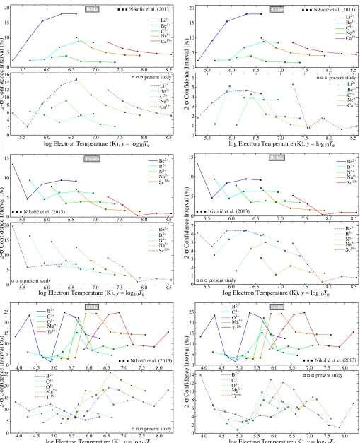
373
Figure 5 illustrates the 2-σ (95.4%) confidence levels in reproducing the suppression factors of
374
Summers (1974 & 1979) for several charge states as a function of electron temperature. Higher
375
electron number densities, for which the three-body recombination becomes a dominant process at
376
low θ values, are excluded from 2-σ estimates. Top panels illustrate the accuracies for select ions
Suppression of Dielectronic Recombination II
Table 4. Values of “detailed”ψN(q, T) and “secondary autoionization”ψN
sec(q, T) given at specifiedN,q, and
T for checking computer code.
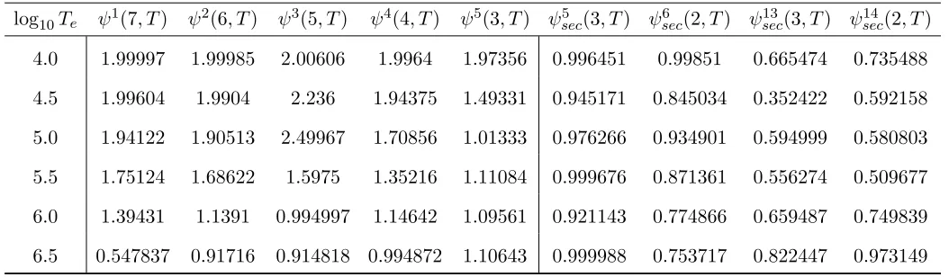
log10Te ψ1(7, T) ψ2(6, T) ψ3(5, T) ψ4(4, T) ψ5(3, T) ψsec5 (3, T) ψsec6 (2, T) ψ13sec(3, T) ψsec14(2, T)
4.0 1.99997 1.99985 2.00606 1.9964 1.97356 0.996451 0.99851 0.665474 0.735488
4.5 1.99604 1.9904 2.236 1.94375 1.49331 0.945171 0.845034 0.352422 0.592158
5.0 1.94122 1.90513 2.49967 1.70856 1.01333 0.976266 0.934901 0.594999 0.580803
5.5 1.75124 1.68622 1.5975 1.35216 1.11084 0.999676 0.871361 0.556274 0.509677
6.0 1.39431 1.1391 0.994997 1.14642 1.09561 0.921143 0.774866 0.659487 0.749839
6.5 0.547837 0.91716 0.914818 0.994872 1.10643 0.999988 0.753717 0.822447 0.973149
using the methodology of Paper I, with adjustment factor Amod,old(N) given in Eq. (8) and Table 1.
378
Bottom panels are corresponding accuracies from the present study: in the left column are results
379
for “simplified” ψ and in the right column for “detailed”ψN(q, T) adjustment factors, both given in
380
Eq. (10) and Table 2. In general, when compared to accuracies of Paper I, the use of “simplified”
381
ψ adjustment factor maintains or slightly improves the accuracy for suppression factors for wide
382
range of temperatures. Most importantly, it removes the discontinuity in suppression factors at
low-383
temperatures as introduced in Paper I for isolectronic sequences below C-like. When activation log
384
densities xa(T;q, N) given in Eq. 3 are evaluated using the “detailed” ψN(q, T) adjustment factors
385
the overall accuracy improves to better than 14 %.
Nikoli´c et al.
5 . 5 6 . 0 6 . 5 7 . 0 7 . 5 8 . 0 8 . 5
0
5
1 0 1 5
2 0 N i k o l i ć e t a l . ( 2 0 1 3 )
C a1 9 +
N e9 +
C 5 +
B e3 +
L i2 +
2 -σ C o n fi d en ce I n te rv al ( % )
H - l i k e
5 . 5 6 . 0 6 . 5 7 . 0 7 . 5 8 . 0 8 . 5
0 2 4 6 8 1 0 1 2 1 4 1 6
p r e s e n t s t u d y
C a1 9 +
N e9 +
C 5 +
B e3 +
L i2 +
l o g E l e c t r o n T e m p e r a t u r e ( K ) , y = l o g 1 0T e
5 . 5 6 . 0 6 . 5 7 . 0 7 . 5 8 . 0 8 . 5
0
5
1 0 1 5
2 0 N i k o l i ć e t a l . ( 2 0 1 3 )
C a1 9 +
N e9 +
C 5 +
B e3 +
L i2 + H - l i k e
5 . 5 6 . 0 6 . 5 7 . 0 7 . 5 8 . 0 8 . 5
0 1 2 3 4 5
6 p r e s e n t s t u d y
C a1 9 +
N e9 +
C 5 +
B e3 +
L i2 +
2 -σ C o n fi d en ce I n te rv al ( % )
l o g E l e c t r o n T e m p e r a t u r e ( K ) , y = l o g 1 0 T e
5 . 5 6 . 0 6 . 5 7 . 0 7 . 5 8 . 0 8 . 5
0
5
1 0 1 5
N i k o l i ć e t a l . ( 2 0 1 3 )
S c1 9 +
N a9 +
N 5 +
B 3 +
B e2 +
2 -σ C o n fi d en ce I n te rv al ( % )
H e - l i k e
5 . 5 6 . 0 6 . 5 7 . 0 7 . 5 8 . 0 8 . 5
0
5
1 0 1 5 2 0
p r e s e n t s t u d y
S c1 9 +
N a9 +
N 5 +
B 3 +
B e2 +
l o g E l e c t r o n T e m p e r a t u r e ( K ) , y = l o g 1 0 T e
5 . 5 6 . 0 6 . 5 7 . 0 7 . 5 8 . 0 8 . 5
0
5
1 0 1 5
N i k o l i ć e t a l . ( 2 0 1 3 )
S c1 9 +
N a9 +
N 5 +
B 3 +
B e2 +
2 -σ C o n fi d en ce I n te rv al ( % )
H e - l i k e
5 . 5 6 . 0 6 . 5 7 . 0 7 . 5 8 . 0 8 . 5
0 1 2 3 4 5 6 7
p r e s e n t s t u d y
l o g E l e c t r o n T e m p e r a t u r e ( K ) , y = l o g 1 0T e
S c1 9 +
N a9 +
N 5 +
B 3 +
B e2 +
4 . 0 4 . 5 5 . 0 5 . 5 6 . 0 6 . 5 7 . 0 7 . 5 8 . 0
0 5 1 0 1 5 2 0 2 5
N i k o l i ć e t a l . ( 2 0 1 3 )
T i1 9 +
M g9 +
O 5 +
C 3 +
B 2 +
2 -σ C o n fi d en ce I n te rv al ( % )
L i - l i k e
4 . 0 4 . 5 5 . 0 5 . 5 6 . 0 6 . 5 7 . 0 7 . 5 8 . 0
0 5 1 0 1 5 2 0 2 5
p r e s e n t s t u d y
T i1 9 +
M g9 +
O 5 +
C 3 +
B 2 +
l o g E l e c t r o n T e m p e r a t u r e ( K ) , y = l o g 1 0 T e
4 . 0 4 . 5 5 . 0 5 . 5 6 . 0 6 . 5 7 . 0 7 . 5 8 . 0
0 5 1 0 1 5 2 0 2 5
N i k o l i ć e t a l . ( 2 0 1 3 )
T i1 9 +
M g9 +
O 5 +
C 3 +
B 2 +
2 -σ C o n fi d en ce I n te rv al ( % )
L i - l i k e
4 . 0 4 . 5 5 . 0 5 . 5 6 . 0 6 . 5 7 . 0 7 . 5 8 . 0
0 2 4 6 8 1 0 1 2
1 4 p r e s e n t s t u d y
T i1 9 +
M g9 +
O 5 +
C 3 +
B 2 +
[image:22.612.62.571.56.683.2]l o g E l e c t r o n T e m p e r a t u r e ( K ) , y = l o g 1 0T e
Figure 5. Estimated accuracy for suppression factors for several charge states as a function of electron
Suppression of Dielectronic Recombination II
4 . 5 5 . 0 5 . 5 6 . 0 6 . 5 7 . 0 7 . 5 8 . 0
0
5
1 0 1 5 2 0
2 5 N i k o l i ć e t a l . ( 2 0 1 3 )
C 2 +
A l9 +
V 1 9 +
F 5 +
N 3 +
C 2 +
A l9 +
V 1 9 +
F 5 +
N 3 +
2 -σ C o n fi d en ce I n te rv al ( % )
B e - l i k e
4 . 5 5 . 0 5 . 5 6 . 0 6 . 5 7 . 0 7 . 5 8 . 0
0
5
1 0 1 5 2 0
2 5 p r e s e n t s t u d y
l o g E l e c t r o n T e m p e r a t u r e ( K ) , y = l o g 1 0T e
4 . 5 5 . 0 5 . 5 6 . 0 6 . 5 7 . 0 7 . 5 8 . 0
0
5
1 0 1 5 2 0
2 5 N i k o l i ć e t a l . ( 2 0 1 3 )
2 -σ C o n fi d en ce I n te rv al ( % )
l o g E l e c t r o n T e m p e r a t u r e ( K ) , y = l o g 1 0 T e
C 2 +
A l9 +
V 1 9 +
F 5 +
N 3 +
C 2 +
A l9 +
V 1 9 +
F 5 +
N 3 + B e - l i k e
4 . 5 5 . 0 5 . 5 6 . 0 6 . 5 7 . 0 7 . 5 8 . 0
0 2 4 6 8 1 0 1 2
1 4 p r e s e n t s t u d y
4 . 5 5 . 0 5 . 5 6 . 0 6 . 5 7 . 0 7 . 5 8 . 0
0 5 1 0 1 5 2 0 2 5
N i k o l i ć e t a l . ( 2 0 1 3 )
B - l i k e
2 -σ C o n fi d en ce I n te rv al ( %
) C r1 9 +
S i9 +
N e5 +
O 3 +
N 2 +
4 . 5 5 . 0 5 . 5 6 . 0 6 . 5 7 . 0 7 . 5 8 . 0
0
5
1 0 1 5 2 0
p r e s e n t s t u d y C rS i1 9 +
9 +
N e5 +
O 3 +
N 2 +
l o g E l e c t r o n T e m p e r a t u r e ( K ) , y = l o g 1 0T e
4 . 5 5 . 0 5 . 5 6 . 0 6 . 5 7 . 0 7 . 5 8 . 0
0 5 1 0 1 5 2 0 2 5
C r1 9 +
S i9 +
N e5 +
O 3 +
N 2 +
C r1 9 +
S i9 +
N e5 +
O 3 +
N 2 +
2 -σ C o n fi d en ce I n te rv al ( % )
B - l i k e
4 . 5 5 . 0 5 . 5 6 . 0 6 . 5 7 . 0 7 . 5 8 . 0
0 2 4 6 8 1 0 1 2
p r e s e n t s t u d y
N i k o l i ć e t a l . ( 2 0 1 3 )
[image:23.612.63.572.52.471.2]l o g E l e c t r o n T e m p e r a t u r e ( K ) , y = l o g 1 0T e
Nikoli´c et al.
Table 5. Fitting coefficients for the excitation energies N(q) = P5j=0pN,j 10q
j
, in eV (see Eq. 16).
Numbers in square brackets denote powers of 10.
Sequence N pN,0 pN,1 pN,2 pN,3 pN,4 pN,5
Li-like 3 1.963[+0] 2.030[+1] -9.710[-1] 8.545[-1] 1.355[-1] 2.401[-2]
Be-like 4 5.789[+0] 3.408[+1] 1.517[+0] -1.212[+0] 7.756[-1] -4.100[-3]
N-like 7 1.137[+1] 3.622[+1] 7.084[+0] -5.168[+0] 2.451[+0] -1.696[-1]
Na-like 11 2.248[+0] 2.228[+1] -1.123[+0] 9.027[-1] -3.860[-2] 1.468[-2]
Mg-like 12 2.745[+0] 1.919[+1] -5.432[-1] 7.868[-1] -4.249[-2] 1.357[-2]
P-like 15 1.428[+0] 3.908[+0] 7.312[-1] -1.914[+0] 1.051[+0] -8.992[-2]
H-, He-, Ne-like 1,2,10 † 0.0 0.0 0.0 0.0 0.0
B-, C-, O-, F-like 5,6,8,9 0.0 0.0 0.0 0.0 0.0 0.0
Al-, Si-, S-, Cl-like 13,14,16,17 0.0‡ 0.0 0.0 0.0 0.0 0.0
≥18 0.0 0.0 0.0 0.0 0.0 0.0
† 20 erfc(2(x−x0
a));
‡ set to 17.6874 for Si-like S2+, seeBadnell et al.(2015).
C. EXCITATION ENERGIESN(Q)
387
With respect to Paper I, we update Table5 with the ion-core excitation energy for Si-like S2+ ion
388
to include the study of Badnell et al. (2015).
Suppression of Dielectronic Recombination II
D. EXAMPLES OF CLOUDY 17 MODEL APPLICATIONS
390
D.1. Elemental Abundances using ψN(q, T) and ψN
sec(q, T) adjustment factors
391
Figure A illustrates finite-density effect on the collisional ionization fractional abundance on all
392
ionization stages of elements up to and including Zn. All results correspond to “detailed” adjustment
393
factor ψN(q, T) given in Eq. (10) and Table2, and where appropriate, to “secondary autoionization”
394
ψN
sec(q, T) adjustment factor given in Eq. (11) and Table 2. The solid and dashed curves in upper
395
panels correspond to electron densities of 1 cm−3 and 1010 cm−3, respectively. From left to right, the
396
curves range from electrically neutral (green) to fully ionized atoms (red). Lower panels in Figure A
397
point to the most effected ionization stages by investigating the ratio of the calculated fractional
398
abundances for the two densities. Similarly, Figure B summarizes finite-density effect at
constant-399
temperature (log10Te = 4.5) on photoionization fractional abundance as a function of ionization
400
parameter log10U.
401
Fig. Set A. collisional ionization fractional abundances 402
Nikoli´c et al.
0 . 0 1 0 . 1 0 1 . 0 0
4 . 0 4 . 5 5 . 0 5 . 5 6 . 0 6 . 5 7 . 0 7 . 5 8 . 0 8 . 5 9 . 0
0 . 1
1
1 0
z i n c
F
ra
c.
A
b
u
n
d
.
D
en
se
/
V
ac
u
u
m
[image:26.612.96.522.62.381.2]l o g E l e c t r o n T e m p e r a t u r e ( K )
Figure A. Upper panels: collisional ionization fractional abundance vs. electron temperature for all
ionization stages of indicated elements. Lower panels: ratio of the calculated fractional abundances for the
Suppression of Dielectronic Recombination II
0 . 0 1 0 . 1 0 1 . 0 0
- 4 . 0 - 3 . 5 - 3 . 0 - 2 . 5 - 2 . 0 - 1 . 5 - 1 . 0 - 0 . 5 0 . 0 0 . 5 1 . 0 1 . 5 2 . 0 2 . 5 3 . 0 3 . 5 4 . 0
0 . 1
1
1 0
z i n c
F
ra
c.
A
b
u
n
d
.
D
en
se
/
V
ac
u
u
m
[image:27.612.99.524.61.383.2]l o g
U
Figure B. Upper panels: photoionization fractional abundance vs. the ionization parameter U for all
ionization stages of indicated elements and for constant temperature log10Te= 4.5. Lower panels: ratio of
the calculated fractional abundances for the two densities. The complete figure set (30 images) is available