A New Interface Identification Technique Based on Absolute Density Gradient for Violent Flows

City, University of London Institutional Repository

Citation: Zhou, Y. & Ma, Q. (2018). A New Interface Identification Technique Based on

This is the accepted version of the paper.

This version of the publication may differ from the final published

version.

Permanent repository link: http://openaccess.city.ac.uk/20256/

Link to published version: http://dx.doi.org/10.3970/cmes.2018.00249

Copyright and reuse: City Research Online aims to make research

outputs of City, University of London available to a wider audience.

Copyright and Moral Rights remain with the author(s) and/or copyright

holders. URLs from City Research Online may be freely distributed and

linked to.

A New Interface Identification Technique Based on Absolute Density

Gradient for Violent Flows

Yan Zhou

_{and Q.W. Ma}

Abstract

An identification technique for sharp interface and penetrated isolated particles is developed for simulating two-dimensional, incompressible and immiscible two-phase flows using meshless particle methods in this paper. This technique is based on the numerically computed density gradient of fluid particles and is suitable for capturing large interface deformation and even topological changes such as merging and breaking up of phases. A number of assumed particle configurations will be examined using the technique, including these with different level of randomness of particle distribution. The tests will show that the new technique can correctly identify almost all the interface and isolated particles, and also show that it is better than other existing popular methods tested.

Keywords:

Meshless method,

1. Introduction

In many engineering problems, such as installation of Deepwater platforms (Wang, Gao and Fang, 2016), one may need to consider two-phase flow. In numerical simulations of two-phase flows, the identification of interface is essential in solving equations describing the transport of momentum, mass and energy. There are various methods for interface identification which can be broadly divided into two groups. One is for mesh-based methods, usually based on an indicator function resulting in an interface with the thickness either covering several grid cells or one cell. The other group is for meshless-based methods, in which particles are moved in Lagrangian formulation, yielding an interface directly which is coincided with the position of a set of particles.

In mesh-based methods, the volume of fluid (VOF) method captures the interface by the indicator function formulated with a volume fraction of either phase. To represent a sharp interface within the mesh, the VOF is often complemented by reconstruction techniques such as piece wise constant approach [Hirt and Nichols (1981); Yokoi (2007)], piecewise linear approach [Aulisa, Manservisi, Scardovelli et al. (2007); Rudman, (1997)], piecewise quadratic [Diwakar, Das and Sundararajan, (2009); Renardy and Renardy, (2002)] or piecewise cubic approximations [Ginzburg and Wittum, (2001); López, Hernández, Gómez et al. (2004)]. To simplify the computational treatment, another way was employed to identify the interface by using a range of the value of a volume fraction [Rudman (1997); Ubbink and Issa (1999); Xiao, Honma and Kono (2005)], which actually represent an interface covering several grid cells. And later Weller [Weller (2008)] and Hoang et al. [Hoang, Steijn, Portela, et al. (2013)] introduced the artificial compression terms to sharpen the interface and counteract the numerical diffusion. Different from artificial geometric representation in the VOF when reconstructing the interface, the indicator in level-set method [Osher and Sethian (1988); Yang, Ouyang, Jiang et al. (2010); Balabel (2012); Balabel (2013)] is a smoothed signed distance function from the interface and zero level-set value gives the location of the interface. To remedy its mass

________________________________

1_{School of Engineering, University of Liverpool, Liverpool L69 3BX, UK}

2School of Mathematics, Computer Science and Engineering, City, University of London, London EC1V 0HB, UK

non-conservation problem, re-initialization for the signed distance function [Min (2010); Sussman and Fatemi (1999)] and mass corrections [Ausas, Dari and Buscaglia (2011); Zhang, Zou and Greaves (2010)] were widely adopted. Phase field method based on free energy theory is also used for interface tracking [Takada, Misawa and Tomiyama (2006); Aland, Lowengrub and Voigt (2010)]. Instead of using Eulerian mesh, the arbitrary Lagrangian-Eulerian mesh system was also adopted in which the unstructured meshes are moved to keep the grid nodes at the interface [Muzaferija and Peri´c (1997); Tukovic and Jasak (2012)].

As for meshless-based methods, the interface can be inherently tracked by moving particles which are initially allocated and remain as one phase during the simulation. For methods that solve two phases in one set of equations based on a smoothed particle hydrodynamics (SPH) method [Hu and Adams (2007); Chen, Zong, Liu et al. (2015); Qiang, Chen and Gao (2011)] and the Moving Particle Semi-implicit (MPS) method [Shakibaeinia and Jin (2012); Khayyer and Gotoh (2013)], interface conditions are implicitly implemented and thus the interface does not need to be explicitly identified. However, for explicit boundary condition implementation, two situations can be observed. One situation is that the flow is not violent or large deformations do not occur, under which particles on the free surface in single phase flows or on the interface of multiphase flows are maintained during the simulation [Ma (2005)], in which the interface is known and its identification is not necessary. The other situation comes with flows being violent or with large deformations and therefore the inner and boundary particles are changeable [Lee, Moulinec, Xu et al. (2008); Ma and Zhou (2009); Shao (2012)], and one phase can penetrates into other phase, forming isolated particles. In this situation, the interface particles and isolated particles (penetrating to the other phase) must be identified in every time step.

In this paper a new interface (and also isolated) particle identification technique is proposed for the meshless-based methods, which is based on absolute density gradient for violent flows. In the next section the existing methods for interface particle identification used in the meshless-based methods will be briefly reviewed. Then the formulation of the new identification technique and parameters tests are given, followed by the comparisons between the new technique and the existing ones. Finally, validations of the new technique on different density ratios, different degree of randomness of particle distribution, various sizes of the support domain in calculating the density gradient and different flow conditions will be carried out.

2. Brief review on interface particle identification techniques for meshless methods

Many applications of meshless methods (e.g. incompressible SPH (ISPH), MPS and MLPG) in single phase wave simulation depend strongly on free surface particle identification based on which the dynamic surface boundary condition can be implemented. A number of approaches have been proposed and adopted in various meshless methods, such as these using the particle number density method (abbreviated to PND) in MPS [Koshizuka, Nobe and Oka (1998); Gotoh and Sakai (2006); Kakuda et al. 2013; Xu and Jin (2014)] and fluid density in ISPH [Shao (2009)]. Both techniques are developed mainly for single phase problems, which lead to lower particle number density (MPS) or lower density (SPH) on the free surface, satisfying Eq. (1) and Eq. (2), respectively

𝑛_𝑖< 𝜃𝑛0 _{( 1 )}

where 𝑛𝑖 = ∑ 𝑤(|𝑟⃗𝑗 𝑗− 𝑟⃗𝑖|) is the particle number density for the target particle 𝑖with w being a weight function and 𝑛0 denotes the inner particle number density which is initially defined. Similar to particle number density, 𝜌𝑖= ∑ 𝑚𝑗 𝑗𝑤(|𝑟⃗𝑗− 𝑟⃗𝑖|) is used to give the estimated density and ρ0 denotes

the specified density of fluid. 𝜃 and 𝜅 are coefficients to evaluate the decreasing of 𝑛𝑖 and 𝜌𝑖 for the interface particles. As pointed by Koshizuka and Oka [Koshizuka and Oka (1996)] the value of 𝜃 could be in the range of 0.8 to 0.99 and was selected as 0.97 in their case study of dam breaking and in modelling weir flows [Xu and Jin (2014)]. 𝑛𝑖 and 𝜅 were chosen as 0.95 for simulating breaking waves on slopes [Koshizuka, Nobe and Oka (1998)] and 0.99 for simulating water entry of a free-fall object [Shao (2009)]. However, this simple approach has been found often to incorrectly identify the interface (or free surface) particles, especially when the particles are unevenly distributed.

As a supplementary to PND, a mixed particle number density and auxiliary function method (MPAM) was proposed [Ma and Zhou (2009)] by additionally counting the existing interface particles and the occupied quarters and rectangles in the support domain in Ma and Zhou [Ma and Zhou (2009)]. The method was further developed by Zheng et al. [Zheng, Ma and Duan (2014)] by defining two quarter-dividing systems and counting the occupied ones in which the value of 𝜅 was chosen as 0.9. As confirmed by many calculations in the cited papers, the accuracy of identifying interface particles is significantly improved with the auxiliary functions. However apart from the complexity in sorting neighbouring particles into quarters and other specific regions, the dependence on the identification of the previous time step could lead to error accumulation once misidentification occurs in previous steps.

Lee et al. [Lee, Moulinec, Xu et al. (2008)] employed a tracking method by estimating the divergence of position vector, 𝑟⃗, with the expression of

(𝛻 ∙ 𝑟⃗)_𝑖 ≈ ∑ ∆𝑉_𝑗(𝑟⃗_𝑗− 𝑟⃗_𝑖)

𝑗

∙ 𝛻𝑤(|𝑟⃗𝑗− 𝑟⃗𝑖|) _{( 3 )}

where ∆𝑉_𝑗 is the volume of the particle associated with particle 𝑗. The value of the numerical

divergence from Eq. (3) is close to 2 for inner particles in two dimensional simulations and decreases on the free surface particles for the reason that the number of neighbouring particles is smaller and the support of the kernel is truncated. Thus the criterion identifying the free surface particles in the cited paper is set as

It was indicated that not all the surface particles were correctly identified and some inner particles are over identified [Lind, Xu, Stansby et al. (2012)] although the misjudgements appeared to be insignificant in the cases they have considered by using the method. Because the theoretical value of the position vector divergence should be 2 for both inner and surface particles, its numerical value should be close to 2 even near or on the interface if more accurate and consistent approximation, such as SFDI gradient scheme (Ma, 2008) is employed to estimate the divergence. From this point of view, the method is questionable for its general use and so will not be considered further in this paper.

Above interface particle identification techniques developed for single phase can be applied in a straightforward way to interface identification in two-phase flows by involving the particles of the other phase if the difference of the two phase densities are large [Shao (2012)] or by neglecting the one phase and picking out the ‘surface’ of the rest phase. To improve the accuracy and reduce the complexity of the interface identification technique, a new approach based on the absolute density

gradient is proposed in this paper. This method is based on the fact that the density gradient is infinite on the interface but zero away from it. In two-phase violent flows, it often happens that one phase penetrates into the other. In that case, the penetrated parts are usually represented by isolated particles for which special treatment are necessary [Gotoh and Sakai (2006)]. Gotoh and Sakai [Gotoh and Sakai (2006)] also provided an identification method using a combination of particle number density and the number of neighbouring particles of the other phase. In comparison the newly proposed technique is able to identify such isolated particles in a more consistent way.

3. Absolute density gradient technique

For immiscible two-phase flows with the sharp density jump at the interface, the density gradients are 0 for inner particles and become theoretically infinite at the interface if both phases are incompressible. For weak compressible phases, the density gradients are close to 0 for inner particles and are also theoretically infinite at the interface. To utilize this fact for interface identification, the absolute value of density gradient is numerically computed as below

𝛽 = |𝜌,𝑥| + |𝜌,𝑦| ( 5)

where

|𝜌,𝑑| =

2

∑ 𝑤(𝑟⃗𝑗 𝑗− 𝑟⃗𝑖)∑|𝜌𝑖

− 𝜌𝑗|

|𝑟𝑗,𝑑− 𝑟𝑖,𝑑|

∆𝑟𝑖𝑗2 𝑤(𝑟⃗𝑗

− 𝑟⃗𝑖) 𝑗

, 𝑑 = 𝑥, 𝑦 _{( 6 )}

and the weight function 𝑤(𝑟⃗𝑗− 𝑟⃗𝑖) is selected as

𝑤(𝑟⃗𝑗− 𝑟⃗𝑖) =

{

1 − 6𝑟2_{+ 8𝑟}3_{− 3𝑟}4 _{𝑟 =}𝑟𝑖𝑗

𝑅_𝑒=

|𝑟⃗_𝑗− 𝑟⃗_𝑖|

𝑅_𝑒 ≤ 1

0 𝑟 =𝑟𝑖𝑗 𝑅𝑒=

|𝑟⃗𝑗− 𝑟⃗𝑖|

𝑅𝑒 > 1

( 7 )

where 𝑟⃗𝑗 and 𝑟⃗𝑖 are the position vectors of neighbour and target particles, 𝑟𝑗,𝑥 and 𝑟𝑗,𝑦 are the

component of 𝑟⃗𝑖 in the 𝑥- and 𝑦- direction, 𝑅𝑒 is the radius of the support domain proportional to ∆𝑙 with ∆𝑙 being the initial average particle distance and ∆𝑟𝑖𝑗 is defined as ∆𝑟𝑖𝑗= 𝑚𝑎𝑥(0.8∆𝑙, |𝑟⃗𝑗− 𝑟⃗𝑖|).

The numerical value of 𝛽 is very close 0 for inner particles and it rapidly increases when approaching to the interface or isolated particles. Although the gradient is theoretically infinite at the interface or isolated particles, it is just a large value in numerical computation.

To obtain a non-dimensional scale of the absolute density gradient 𝛽₀ is introduced with the expression of

𝛽₀= |𝜌₁− 𝜌₂|/∆𝑙 ( 8 )

horizontal or vertical interfaces, 1.0 for diagonal interfaces and 2.0 for isolated particles by using Eq. ( 5) and ( 6 ). It is noted here that for any distribution of particles with the weight function given by Eq. ( 7 ) and a fixed support domain size, the value of 𝛽/ 𝛽0 remains independent on the value of ∆𝑙. It is also noted that the value of 𝛽/ 𝛽₀ will not be affected by the density ratio of the two phases. In other words, the value of 𝛽/ 𝛽0 is independent on the total number of particles for a given domain and density ratio. Nevertheless, in general situations with the particular weight function used and the chosen radius of the support domain, the value of 𝛽/ 𝛽0will vary in a range with the change of particle distribution. Therefore the most suitable values need to be determined by considering a range of flowing conditions of the two phases. The following two conditions (I) and (II) are then checked.

(I) 𝛾 < 𝛽 𝛽⁄ ₀< 𝛼 ( 9a)

(II) 𝛽 𝛽⁄ 0≥ 𝛼 ( 9b)

If Condition (I) is satisfied, the particles are identified to be interface particles. If Condition (II) is met, the particles are identified as isolated particles. If none of the conditions is satisfied, they are classified as inner particles. For general cases, particles move and become irregularly distributed. The values of γ and 𝛼 will be discussed below using numerical tests. This approach based on Eqs. (5) to (9) is shortened as ADG (absolute density gradient) method hereafter for convenience.

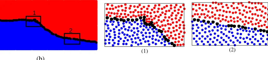
To determine the value of 𝛾and 𝛼, a number of tests are carried out for a specified particle configurations shown in Fig. 1. In this figure, two typical regions are enlarged. Particles are clustered in region 1 and relatively coarser in region 2. As shown in Fig. 1(a), an under-specified value of 𝛾 (e.g. 0.1), leads to misidentifying inner particles close to the interface in the clustered region (some inner particles are identified as interface particles, i.e., over-identified). However, an over-specified value of

𝛾 (e.g. 0.5), shown in Fig. 1(b), leads to missing the particles on the interface in the region where the distribution of particles is relatively coarser (i.e., under-identified). Based on this, we can deduce that there might be a range of values for 𝛾 which may lead to correctly identifying the interface particles. We have also tested the value of 𝛾 in the range of 0.2 to 0.4 for the same configuration and found that the interface particles are correctly picked out and insensitive to the specific value in the range. The results of 𝛾 = 0.2 and 𝛾 = 0.4 are illustrated in Fig. 2. Hereafter, the value of 𝛾 is selected to be 0.3, unless mentioned otherwise. It is noted here that the new scheme discussed above will not misidentify the inner particles away from interface as the value of 𝛽/ 𝛽₀ is always zero or very close to zero for incompressible and weak compressible fluids. When the value of 𝛾 is smaller, it tends to be that more particles near the interface may be misidentified as interface particle (e.g., Fig. 1(a)). However, this kind of misidentification will not significantly affect the computation results as the values of physical variables near the interface are very close to those on the interface. More discussions about this point may be found in Ma and Zhou [Ma and Zhou (2009)].

(a)

1

2

(b)

Figure 1: Examples of interface identifications when applying improper values of 𝜸. (a) shows inner particles close to the

interface are over-identified with 𝜸 = 𝟎. 𝟏 and (b) shows some interface particles are under-identified with 𝜸 = 𝟎. 𝟓. (density ratio: 1:1000)

(a)

(b)

Figure 2: Examples of interface identifications when applying proper values of 𝜸. (a) shows the interface identified by 𝜸 =

𝟎. 𝟐 and (b) is obtained by 𝜸 = 𝟎. 𝟒. (density ratio: 1:1000)

Another particle configuration associated with the violent sloshing of two phases is used to illustrate the effects of value for 𝛼 in Condition (II). Fig. 3(a) and (b) show that the isolated particles penetrating into the other phase are identified by using the value of 𝛼 to be 1.4 and 1.6, respectively. It can be seen that the isolated particles of both phases are correctly identified by using either value. This demonstrates that the results are not sensitive to the value of 𝛼 when it is within the range of 1.4 to 1.6. Thus 𝛼=1.5 will be used for isolated particle identification.

(a) 2

1

(1) (2)

2

1

(1) (2)

1

2

(b)

Figure 3: Isolated particles marked by squares for heavier fluid particles and diamonds for lighter fluid particles (density

ratio: 1:1000) are identified with 𝛂being 1.4 (a) and 1.6 (b). The heavier phase is marked in black and the lighter is in light grey. In the enlarged figures on the right, support domains for each isolated particles are marked with a circle.

According to above numerical tests, the values of 𝛾 and 𝛼are selected to be 0.3 and 1.5 for the conditions of (I) and (II) to identify the interface particles and isolated particles, respectively.

4. Validations

4.1 Identification with different random distributions of particles

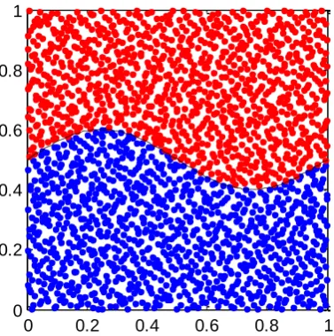
The newly proposed interface identification technique will be further validated on random distributed particles. Comparison will be made with the results of other two methods. One is the PND method used by MPS simulation and the other is the MPAM [Ma and Zhou (2009)] as mentioned in Section 2. The tests are first carried out on the specified configuration shown in Fig. 4 in which the unit patch is divided into two portions by a sinusoidal curve of 𝑦 = 0.1𝑠𝑖𝑛(2𝜋𝑥) + 0.5. Particles are randomly distributed by using the ‘haltonset’ function available in MATLAB. Below the sinusoidal curve the particles represent the fluid phase 1 (blue dots) and the rest is filled by fluid phase 2 (red dots).

Figure 4: Sketch of interface testing case. 2000 random distributed particles in a unit patch divided into two portions by 𝒚 =

𝟎. 𝟏𝒔𝒊𝒏(𝟐𝝅𝒙) + 𝟎. 𝟓 shown by dashed line. Blue and red dots represent the fluid phase 1 and fluid phase 2, respectively.

0 0.2 0.4 0.6 0.8 1

(a) (b)

(c) (d)

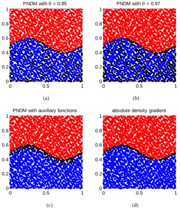
Figure 5: Interface particles (black nodes) identification by PND with 𝜽 = 𝟎. 𝟖𝟓 (a), PND with 𝜽 = 𝟎. 𝟗𝟕(b), PND with

auxiliary functions (c) and ADG (d). Blue and red dots represent the fluid phase 1 and fluid phase 2 respectively. (Density ratio=0.9)

(a) (b) (c)

Figure 6: Interface particles (black nodes) identification by PND with 𝜽 = 𝟎. 𝟖 (a), 𝜽 = 𝟎. 𝟕(b) and 𝜽 = 𝟎. 𝟔 (c). Blue and

red dots represent the fluid phase 1 and fluid phase 2, respectively.

When using the PND and MPAM methods, interface particles are identified as surface particles of the phase 1 by ignoring the present of the phase 2 as they are developed for single phase problem. As shown in Fig. 5 black dots are the interface particles identified by the PND method with 𝜃 = 0.85 and

0 0.5 1

0 0.2 0.4 0.6 0.8 1

PNDM with  = 0.85

0 0.5 1

0 0.2 0.4 0.6 0.8 1

PNDM with  = 0.97

0 0.5 1

0 0.2 0.4 0.6 0.8 1

PNDM with auxiliary functions

0 0.5 1

0 0.2 0.4 0.6 0.8 1

absolute density gradient

0 0.5 1

0 0.2 0.4 0.6 0.8 1

PNDM with  = 0.8

0 0.5 1

0 0.2 0.4 0.6 0.8 1

PNDM with  = 0.7

0 0.5 1

0 0.2 0.4 0.6 0.8 1

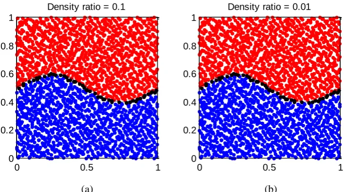
𝜃 = 0.97 in Fig. 5(a) and (b), which are in the range of 𝜃 proposed by Koshizuka and Oka [Koshizuka and Oka (1996)]. One can observe that the interface particles are highly over-identified with many inner particles are marked as interface ones although it is moderately relieved by decreasing the coefficient. Such over-identification was also observed by Zheng et al. [Zheng, Ma and Duan (2014)] in their dam breaking simulation. There are also several particles located on the interface but not identified by using either value of 𝜃. Other 𝜃 values are also tested and the results are shown in Fig. 6. One can find that decreasing the value helps alleviate over-identification of inner particles but more interface particles are also missed. The reasons for such inaccuracy are that the accuracy of the PND method strongly depends on the randomness of the particle distribution [Ma and Zhou (2009)]. For inner particles, coarse distribution leads to low particle number density even with a complete support domain and so over-identification happens. On the contrast, particles clustering on the interface leads to high particle number density even though the support domain of its own phase is incomplete, leading to their misidentification to inner particles. For the results obtained using the MPAM shown in Fig. 5(c), the accuracy is significantly improved. But over-identification still happens on inner particles close to the interface. Since this identification technique is based on the interface particles identified at the previous time step, error accumulation may occur after long time simulation. Fig. 5(d) shows the results obtained by the method proposed in this paper. It can be seen that almost all the interface particles are correctly identified. No inner particles are wrongly identified by the method. As indicated above, the new technique does not depend on the density ratio. To confirm this, the tests are also carried out on different density ratios of 0.1 and 0.01 in addition to the ratio of 0.9 in Fig. 5(d) by using the ADG method, and the results for the density ratios of 0.1 and 0.01are shown in Fig. 7. This figure and Fig. 5(d) show that the accurate identification is achieved in all the cases, demonstrating that results of the ADG method are independent of the density ratios.

(a) (b)

Figure 7: Interface particles (black nodes) identification by ADG technique on density ratios of 0.1 with the densities of blue

and red dots of 10 and 1 respectively in (a) and 0.01 with the densities of blue and red dots of 100 and 1 respectively in (b).

In modelling violent multiphase flow, the particle distribution can become very random even they are uniformly distributed initially. It is important to examine the behaviours of interface identification methods at different levels of randomness of particle distributions. For this purpose, we use a configuration similar to that in Fig. 4 with a particle number of 2500; however the particles are

distributed in a way that they are first uniformly located and then deviated by ∆𝑟⃗ = 𝑘 [(𝑅_𝑛𝑥−

0 0.5 1

0 0.2 0.4 0.6 0.8 1

Density ratio = 0.1

0 0.5 1

0 0.2 0.4 0.6 0.8 1

0.5)𝑒⃗𝑥+ (𝑅_𝑛𝑦− 0.5) 𝑒⃗𝑦] ∆𝑙, i.e., the position of particle is given by 𝑟⃗ = 𝑟⃗0+ ∆𝑟⃗ , where each of 𝑅_𝑛𝑥 and 𝑅_𝑛𝑦 is a group of random numbers ranging from 0 to 1.0 generated separately in 𝑥- and 𝑦-

direction, respectively;𝑘is the randomness coefficient and ∆𝑙is the particle distance in uniform distribution; 𝑒⃗𝑥 and 𝑒⃗𝑦 are the unit vector in 𝑥- and 𝑦-direction, respectively; 𝑘 = 0 leads to zero

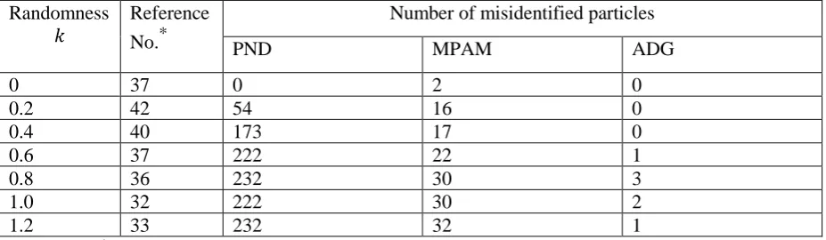
deviation and uniform distribution. As 𝑘 increases, the distribution becomes more disorderly. If the value of 𝑘 is equal to or large than 1, there would be possibility that the position of a particle can be shifted by more than ∆𝑙. The three methods (PND, MPAM and ADG) are employed to identify the interface particles for the cases with different level of randomness. The numbers of particles inaccurately identified for three techniques are listed in Tab. 1 with 𝑘 increasing from 0 to 1.2. The reference number is the number of particles on the interface, which are at or near the specified interface curve within the distance of 0.5∆𝑙. One can see that the number of misidentified particles by the PND method is small only when the value of 𝑘 is very small but with the increase of the 𝑘 value (level of randomness), the number of misidentified particles are large, even much larger than the number of interface particles. In contrast, the number of misidentified particles for each value of 𝑘by the MPAM is significantly reduced but is still considerable. Comparatively, the number of misidentification by the ADG method is very small and not increases with the increase of randomness. To have a clearer look at their performances, the ratio of inaccurate identification defined as the number of misidentified particles divided by the reference number is demonstrated in Fig. 8. It shows that, by increasing the randomness, more than 7 times of the interface particles are misidentified by the PND when 𝑘 reaches 1.2 while this ratio decreases to 0.97 with more moderate incensement by the MPAM. The maximum ratio is less than 0.09 arising at 𝑘 = 0.8 and shows less dependency on the value of 𝑘 by the ADG. With the same configuration, the total particle numbers of 900, 1600, 2500, 3600, 4900 and 6400 are also tested using the ADG method with the values of 𝑘 =

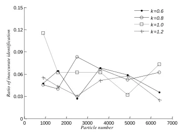
0.6, 0.8, 1.0 and 1.2. The results are given in Fig. 9, showing that the performance of the ADG technique is insensitive to the total particle number. This observation is consistent with what is mentioned previously that the technique does not depend on the average distance between particles. The slight change in the results showing in Fig. 9 is due to random distribution of particles.

Table 1: The number of misidentified particles for different particle distribution randomness by using PND, MPAM and ADG methods

Randomness

𝑘 Reference _No.*

Number of misidentified particles

PND MPAM ADG

0 37 0 2 0

0.2 42 54 16 0

0.4 40 173 17 0

0.6 37 222 22 1

0.8 36 232 30 3

1.0 32 222 30 2

1.2 33 232 32 1

Figure 8: The ratios of inaccurate identification (number of misidentified particles/the reference number) of increasing randomness by using three identification techniques.

Figure 9: The ratios of inaccurate identification (number of misidentified particles/the reference number) of increasing total

particle number using the method of ADG with randomness coefficients of 0.6 to 1.2

Tests are also carried out for various support domain sizes 𝑅𝑒 of the weight function within the range of1.4∆𝑙 to 4.0∆𝑙 which is widely adopted for function interpolation, gradient and Laplacian approximations [Ataie-Ashtiani and Farhadi (2006); Gotoh and Fredsøe (2000); Xu and Jin (2014); Zheng, Ma and Duan (2014)]. Following the above setup for 𝑘 = 0.6 and 1.0, the numbers of misidentified particles by the ADG are listed in Tab. 2. It shows that small support domain (e.g.𝑅_𝑒/

0 0.2 0.4 0.6 0.8 1 1.2

0 1 2 3 4 5 6 7 8 Randomness k R a ti o o f in a c c u ra te i d e n ti fi c a ti o n PND

PND with auxiliary functions Absolute Density Gradient

0 1000 2000 3000 4000 5000 6000 7000

∆𝑙 = 1.4 and 1.6) leads to moderate increment of misidentification due to insufficient neighbouring particles to accurately estimate the density gradient. By increasing 𝑅𝑒/∆𝑙(>2.1), the results become insensitive to the variation of the size and even better. Considering the computational time, 𝑅𝑒/∆𝑙 =

2.1 as selected in above tests is reasonable, but one can choose to use a larger support domain for identifying the interface particles.

Table 2: Numbers of misidentified particles by the ADG method with different support domain size

Re for two values of k = 0.6 and 1.0

𝑅_𝑒/∆𝑙 1.4 1.6 1.8 2.1 2.5 3.0 3.5 4.0

𝑘 = 0.6 7 6 2 1 0 0 0 0

𝑘 = 1.0 8 6 3 2 1 1 0 0

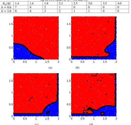
(a) (b)

(c) (d)

Figure 10: Black dots and filled diamonds are interface and isolated particles identified by the ADG technique in four dam

breaking snapshots. The heavier fluid with the density of 1.0 of phase 1 is represented by blue dots and the lighter fluid with density of 0.001 of phase 2 is represented by red dots.

4.2 Identifications for the dam breaking flow

To further validate the newly proposed identification technique on different flow conditions, four snapshots are picked from a dam breaking simulation [Zheng, Ma and Duan (2014)], in which the heavier fluid (phase 1-water) indicated by blue dots is released in the lighter fluid (phase 2 – air)

0 0.5 1 1.5 2

0 0.5 1 1.5

0 0.5 1 1.5 2

0 0.5 1 1.5

0 0.5 1 1.5 2

0 0.5 1 1.5

0 0.5 1 1.5 2

indicated by red dots. The four configurations shown in Fig. 10 include the changing and irregular shape of the released water with a smooth interface in (a), a backward jet in (b), the jet merging into the bottom water in (c) and a second jet in (d). A trapped air bubble also appears in (c) and (d). The density ratio of the two phases in this test is 1:1000. As we can observe from Fig. 10, the interface and isolated particles (black dots) are accurately identified for all the configurations, indicating that the ADG method works well for the more complex cases.

5. Conclusion

This paper has presented a new interface particle identification method for violent two-phase flows based on the absolute density gradient (ADG). The behaviour of the method is tested for different configurations including these with different level of randomness. It is shown that the accuracy of the method is independent of the density ratio of two phases and of the average distance between particles. In all the cases tested, the method can correctly pick up almost all the interface and isolated particles as long as the support domain is larger than twice average distance of particles.

Acknowledgement

The authors gratefully acknowledge the PhD scholarship provided to Y Zhou by City University and China Scholarship Council and the financial support of the EPSRC through its research grants (EP/N008863/1, EP/M022382/1).

References

Aland, S.; Lowengrub, J.; Voigt, A. (2010): Two-phase flow in complex geometries: A diffuse domain approach. Computer Modeling in Engineering & Sciences, vol. 57, no. 1, pp. 77-106.

Ataie-Ashtiani, B.; Farhadi, L. (2006). A stable moving-particle semi-implicit method for free surface flows. Fluid Dynamics Research, vol. 38, no. 4, pp. 241-256.

Aulisa, E.; Manservisi, S.; Scardovelli, R.; Zaleski, S. (2007): Interface reconstruction with least-squares fit and split advection in three-dimensional Cartesian geometry. Journal of Computational Physics, vol. 225, no. 2, pp. 2301-2319.

Ausas, R. F.; Dari, E. A.; Buscaglia, G. C. (2011): Ageometric mass-preserving redistancing scheme for the level set function Roberto. International Journal for Numerical Methods in Fluids, vol. 65, no. 8, pp. 989-1010.

Balabel, A. (2013): Numerical Modelling of Liquid Jet Breakup by Different Liquid Jet/Air Flow Orientations Using the Level Set Method. Computer Modeling in Engineering & Sciences, vol. 95, no. 4, pp.283-302.

Balabel, A. (2012): Numerical Modelling of Turbulence Effects on Droplet Collision Dynamics using the Level Set Method. Computer Modeling in Engineering & Sciences, vol. 89, no. 4, pp. 283-301.

Chen, Z.; Zong, Z.; Liu, M. B.; Zou, L.; Li, H. T.; Shu, C. (2015): An SPH model for multiphase flows with complex interfaces and large density differences. Journal of Computational Physics, vol. 283, pp. 169-188.

Physics, vol. 228, no.24, pp. 9107-9130.

Ginzburg, I.; Wittum, G. (2001): Two-Phase Flows on Interface Refined Grids Modeled with VOF, Staggered Finite Volumes, and Spline Interpolants. Journal of Computational Physics, vol. 166, no. 2, pp. 302-335.

Gotoh, H.; Fredsøe, J. (2000): Lagrangian Two-Phase Flow Model of the Settling Behavior of Fine Sediment Dumped into Water. 27th International Conference on Coastal Engineering, Sydney, Australia, pp. 3906-3919.

Gotoh, H.; Sakai, T. (2006). Key issues in the particle method for computation of wave breaking.

Coastal Engineering, vol. 53, no. 2-3, pp. 171-179.

Qiang, H. F.; Chen, F. Z.; Gao, W. R. (2011): Modified Algorithm for Surface Tension with Smoothed Particle Hydrodynamics and Its Applications. Computer Modeling in Engineering & Sciences, vol. 77, no. 4, pp. 239-262.

Hirt, C. W.; Nichols, B. D. (1981). Volume of fluid (VOF) method for the dynamics of free boundaries. Journal of Computational Physics, vol. 39, no. 1, pp. 201-225.

Hoang, D. A.; Steijn, V.; Portela, L. M.; Kreutzer, M. T.; Kleijn, C. R. (2013): Benchmark numerical simulations of segmented two-phase flows in microchannels using the Volume of Fluid method. Computers and Fluids, vol. 86, pp. 28-36.

Hu, X. Y.; Adams, N. A. (2007): An incompressible multi-phase SPH method. Journal of Computational Physics, vol. 227, no.(1), pp. 264-278.

Khayyer, A.; Gotoh, H. (2013): Enhancement of performance and stability of MPS mesh-free particle method for multiphase flows characterized by high density ratios. Journal of Computational Physics, vol. 242, pp. 211-233.

Koshizuka, S.; Nobe, A.; Oka, Y. (1998): Numerical analysis of breaking waves using the moving particle semi-implicit method. International Journal for Numerical Methods in Fluids, vol. 26, no. 7, pp. 751-769.

Koshizuka, S.; Oka, Y. (1996): Moving-particle semi-implicit method for fragmentation of incompressible fluid. Nuclear Science and Engineering, vol. 123, no. 3, pp.421-434.

Lee, E. S.; Moulinec, C.; Xu, R.; Violeau, D., Laurence, D.; Stansby, P. (2008): Comparisons of weakly compressible and truly incompressible algorithms for the SPH mesh free particle method.

Journal of Computational Physics, vol. 227, no. 18, pp. 8417-8436.

Lind, S. J.; Xu, R.; Stansby, P. K.; Rogers, B. D. (2012): Incompressible smoothed particle hydrodynamics for free: surface flows: A generalised diffusion-based algorithm for stability and validations for impulsive flows and propagating waves. Journal of Computational Physics, vol. 231, no. 4, pp. 1499-1523.

López, J.; Hernández, J.; Gómez, P.; Faura, F. (2004): A volume of fluid method based on multidimensional advection and spline interface reconstruction. Journal of Computational Physics, vol. 195, no. 2, pp. 718-742.

Ma, Q. W. (2005): MLPG Method Based on Rankine Source Solution for Simulating Nonlinear Water Waves. Computer Modeling in Engineering and Sciences, vol. 9, no. 2, pp. 193-209.

Ma, Q. W. (2008): A New Meshless Interpolation Scheme for MLPG_R Method. Computer Modeling in Engineering and Sciences, vol. 23, no. 2, pp. 75-89.

Ma, Q. W.; Zhou, J. T. (2009): MLPG_R Method for Numerical Simulation of 2D BreakingWaves.

CMES - Computer Modeling in Engineering and Sciences, vol. 43, no. 3, pp. 277-303.

Muzaferija, S.; Peri´c, M. (1997): Computation of Free-Surface Flows Using the Finite-Volume Method and Moving Grids. Numerical Heat Transfer, Part B: Fundamentals, vol. 32, no. 4, pp. 369-384.

Osher, S.; Sethian, J. A. (1988): Fronts propagating with curvature dependent speed: Algorithms based on Hamilton-Jacobi formulations. Journal of Computational Physics, vol. 79, pp. 12-49.

Rafiee, A.; Cummins, S.; Rudman, M.; Thiagarajan, K. (2012): Comparative study on the accuracy and stability of SPH schemes in simulating energetic free-surface flows. European Journal of Mechanics, B/Fluids, vol. 36, pp. 1-16.

Renardy, Y.; Renardy, M. (2002): PROST: A Parabolic Reconstruction of Surface Tension for the Volume-of-Fluid Method. Journal of Computational Physics, vol. 183, no. 2, pp. 400-421.

Rudman, M. (1997): Volume-Tracking Methods for Interfacial Flow Calculations. International Journal for Numerical Methods in Fluids, vol. 24, no.7, pp. 671-691.

Shakibaeinia, A.; Jin, Y. (2012): Lagrangian multiphase modeling of sand discharge into still water.

Advances in Water Resources, vol. 48, pp. 55-67.

Shao, S. D. (2009): Incompressible SPH simulation of water entry of a free-falling object.

International Journal for Numerical Methods in Fluids, vol. 59, pp. 59-115.

Shao, S. D. (2012): Incompressible smoothed particle hydrodynamics simulation of multifluid flows.

International Journal for Numerical Methods in Fluids, vol. 69, pp. 1715-1735.

Sussman, M.; Fatemi, E. (1999): An Efficient, Interface-Preserving Level Set Redistancing Algorithm and Its Application to Interfacial Incompressible Fluid Flow. SIAM Journal on Scientific Computing, vol. 20, no.4, pp. 1165-1191.

Takada, N.; Misawa, M.; Tomiyama, A. (2006): A phase-field method for interface-tracking simulation of two-phase flows. Mathematics and Computers in Simulation, vol. 72, no. 2–6, pp. 220-226.

Tukovic, Z.; Jasak, H. (2012): A moving mesh finite volume interface tracking method for surface tension dominated interfacial fluid flow. Computers and Fluids, vol. 55, pp. 70-84.

Ubbink, O.; Issa, R. I. (1999): A Method for Capturing Sharp Fluid Interfaces on Arbitrary Meshes.

Journal of Computational Physics, vol. 153, no. 1, pp. 26-50.

Weller, H. G. (2008): A New Approach to VOF-based Interface Capturing Methods for Incompressible and Compressible Flow. Technical Report TR/HGW/07, OpenCFD Ltd.

Xiao, F.; Honma, Y.; Kono, T. (2005): A simple algebraic interface capturing scheme using hyperbolic tangent function. International Journal for Numerical Methods in Fluids, vol. 48, no. 9, pp. 1023-1040.

Xu, T.; Jin, Y. (2014). Numerical investigation of flow in pool-and-weir fishways using a meshless particle method. Journal of Hydraulic Research, vol. 52, no.6, pp. 849-861.

Yang, B.; Ouyang, J.; Jiang, T.; Liu, C. (2010): Modeling and Simulation of Fiber Reinforced Polymer Mold Filling Process by Level Set Method. Computer Modeling in Engineering & Sciences, vol. 63, no. 3, pp. 191-222.

Yokoi, K. (2007): Efficient implementation of THINC scheme: A simple and practical smoothed VOF algorithm. Journal of Computational Physics, vol. 226, no. 2, pp. 1985-2002.

Zhang, Y.; Zou, Q.; Greaves, D. (2010): Numerical simulation of free-surface flowusing the level-set method with global mass correction Yali. International Journal for Numerical Methods in Fluids, vol. 63, pp. 651-680.

-314.