Analysis of responsive satellite manoeuvres using graph theoretical techniques

IWSCFF 19-32

ANALYSIS OF RESPONSIVE SATELLITE MANOEUVRES

USING GRAPH THEORETICAL TECHNIQUES

Ciara N. McGrath,

Ruaridh A. Clark,

and Malcolm Macdonald

Manoeuvrable, responsive satellite constellations that can respond to real-time events could provide critical data on-demand to support, for example, disaster monitoring and relief efforts. The authors demonstrate the feasibil-ity of such a system by expanding on a fully-analytical method for designing responsive spacecraft manoeuvres using low-thrust propulsion. This method enables responsive manoeuvre planning to provide coverage of targets on the Earth, with each manoeuvre option having a different target look angle, and requiring a different manoeuvre time and propellant cost. The trade-space for this analysis rapidly expands when considering multiple trade- space-craft, targets and manoeuvres. To explore the trade-space efficiently, it is perceived as a graph in which connections are rapidly traversed to identify favourable routes to achieve the mission goals. The case study presented considers four satellites required to provide flyovers of two targets, with an associated graph of possible manoeuvres comprising 10726 nodes. The min-imum time solution is 2.59 days to complete both flyovers with 7.037 m/s change in velocity. Investigation of the graph highlights that selecting a good but not minimum time solution can allow the system to perform well but also have alternate options available to deal with possible errors in the manoeuvre execution, or changes in mission priorities. Restricting the prob-lem to consider only two satellites, with a smaller swath and less available propellant, reduces the graph to 510 nodes. In this case, the minimum time solution requires 9.04 m/s velocity change and takes approximately 2.59 days. The analysis also provides non-intuitive solutions, for example, that it is faster for one satellite to perform two targeting manoeuvres than for two satellites to manoeuvre simultaneously.

INTRODUCTION

Interest in the use of responsive satellite systems is growing as terrestrial applications in-creasingly necessitate the use of real-time, on-demand data1, 2, 3. Current state-of-the-art satel-lite systems, such as those operated by Planet, Inc.4 and Spire Global, Inc.5, 6, cannot manoeu-vre and, as such, would require thousands of satellites to meet this future demand; this is both impractical and financially prohibitive with potentially severe implications for our already congested space environment7, 8. Successful implementation of manoeuvrable satellite sys-tems will address this issue by reducing the number of spacecraft needed to provide

*

Research Associate, Department of Mechanical and Aerospace Engineering, University of Strathclyde, 16 Rich-mond St, Glasgow G1 1XQ, [email protected].

†

Research Associate, Department of Mechanical and Aerospace Engineering, University of Strathclyde, 16 Rich-mond St, Glasgow G1 1XQ, [email protected].

‡

demand information for time-critical applications, such as disaster response. However, to en-sure efficient operation of such a system, an understanding of the capabilities and limitations of manoeuvrable spacecraft is required, as is a method for analysing and comparing the multi-tude of distinct manoeuvre options.

Previous research by the authors has developed a fast and accurate method of planning spacecraft manoeuvres using low-thrust propulsion that can facilitate rapid analysis of respon-sive scenarios involving numerous satellites, targets, and ground stations 9, 10. This method uses general perturbation techniques and thus can produce a large number of solutions ex-tremely quickly whilst maintaining a high degree of accuracy. The method can provide the user with a full overview of all the eligible manoeuvre options for flying over a region of in-terest on the Earth. These options will vary in terms of the change in velocity, or ΔV, required for the manoeuvre, as well as the time taken for the manoeuvre and the look-angle to the tar-get at flyover. As such, the ability to consider all options is extremely valuable, allowing the operator to trade-off each solution and identify those that best align with their unique mission priorities. This previous work demonstrated that reconfiguring a constellation of 24 satellites could provide increased persistence of coverage of 1.6 – 10 times compared to a traditional, non-manoeuvring constellation, depending on the latitude of the target region. For the scenar-io considered, it was predicted that up to 12 targeting reconfiguratscenar-ions could be performed. However, these prior analyses selected the reconfiguration manoeuvres by considering each reconfiguration independently; in fact, manoeuvres selected early in the mission will affect the choices available in the future and thus, for truly efficient operations, a long-term assess-ment is required, considering the full sequence of manoeuvres necessary to achieve the mis-sion goals.

This article addresses the challenge of long-term manoeuvre planning for responsive spacecraft constellations by using the previously developed method of low-thrust spacecraft manoeuvre propagation to create an expansive space of manoeuvre options. This trade-space is represented as a graph that can be explored to obtain insights into the capabilities of the responsive system and to devise a concept of operations that considers the entire opera-tional scenario. The use of the previously derived fast method of manoeuvre calculation al-lows for large graphs encompassing thousands of manoeuvres to be generated.

A graph capturing all possible manoeuvre options, where each option is represented as an edge, can comprise of many of thousands of nodes that each represent a flyover target. When edges are supplied with a weighting that captures some property of a manoeuvre, such as time taken or ΔV required, then an optimal path through the graph can emerge. Manually identify-ing effective routes in large graphs is not always feasible, but shortest path algorithms, such as Dijkstra’s algorithm, can efficiently identify these paths to inform manoeuvre decisions. Shortest path is a useful but limited metric, especially when considering a responsive satellite system, where a shortest path might become unusable given the potential for errors in the first manoeuvre or where the mission priorities might shift in a rapid response scenario. Therefore, a different route through the graph that presents many good options rather than a single opti-mal option may be preferable. The graph enables a trade-off between finding a short route through the graph and ensuring that there are many good options if the route needs to be al-tered due to changing mission priorities or the expected satellite position.

METHOD

Problem Statement

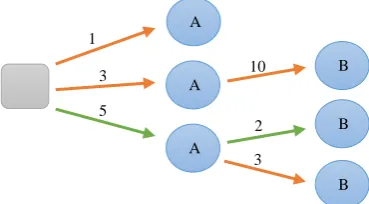
To understand the motivation behind this work, first consider a single, manoeuvrable satel-lite that is required to sequentially fly over two targets, A and B. There are a multitude of ma-noeuvres that can be employed to flyover the targets, each with a different ΔV cost, manoeu-vre time, and resultant look angle to the target9. Ultimately, the choice of manoeuvre places the satellite in a different location within its orbit, which will then affect the next decision. This is presented in Figure 1 where each possible flyover of each target is considered as dis-tinct, due to the difference in orbit parameters at the time of flyover.

In Figure 1, there are three possible manoeuvre options for flying over target A and the re-quired ΔV is indicated for each manoeuvre. For the purposes of this example, minimising ΔV is the only operational goal; manoeuvre time and look angle at flyover are also considered but only in terms of providing operational constraints (e.g. maximum values allowable), such that the manoeuvres shown are those that meet the selected criteria. Consider the first manoeuvre to flyover target A; in considering this stage of manoeuvring alone, it is clear that the upper-most manoeuvre, requiring 1 m/s ΔV, is the minimum ΔV manoeuvre. However, from this point there is no suitable manoeuvre available to provide a subsequent flyover of target B. The central manoeuvre to flyover target A requires 3 m/s ΔV and is the next best manoeuvre for the first stage. However, considering the next manoeuvre to flyover target B, there is only one option available and this has a very high ΔV cost. Indeed, in this scenario, choosing the highest ΔV manoeuvre for the first stage to flyover target A will minimise the ΔV required for the full scenario. The minimum ΔV path for this scenario is shown in green in Figure 1. This illustrates the need to consider the full operational scenario, rather than selecting ma-noeuvres for each stage of the mission independently.

Figure 1: Scenario for sequential flyover of targets A then B from an initial system state, with each possible manoeuvre option represented by a single arrow. Numbers represent the ΔV re-quired for each manoeuvre. The minimum ΔV path is shown in green.

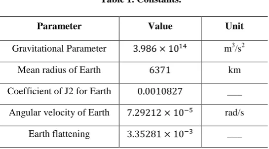
A more complex scenario can be envisaged, in which two satellites are available to ma-noeuvre and flyover two targets, A and B, but the flyovers can occur in any order. Satellite 1 or 2 could flyover both targets, in either order, or each satellite could flyover one target each. Additionally, for each manoeuvre there are a variety of possible options, which differ in ΔV, manoeuvre time and look angle to target at flyover; this is visualised in Figure 2. It is clear that this presents a greater challenge than the example previously presented, though it is much simpler than the operational scenarios expected of a real responsive constellation.

A

B A

A 1

3

5

B

B 10

2

Figure 2: Scenario where two satellites can flyover targets A and B in any order, with each possi-ble manoeuvre option represented by a single arrow. Numbers represent the ΔV required for each manoeuvre.

Representing the Scenario as a Graph

In order to consider all the possible options to complete the task of flying over multiple targets, in any order, with multiple spacecraft available for tasking, it is helpful to visualise the scenario as a graph. This is similar to the decision trees shown in Figure 2, where the pos-sible flyovers of each target can be considered as nodes and the manoeuvres can be consid-ered as edges. However, the representation used in Figure 2 produces one graph for each sat-ellite; this makes concurrent analysis considering all satellites and targets challenging.

In order to create a single graphical representation of the scenario, the location of all tar-gets of interest are defined in terms of their latitude and longitude. The initial positions of all satellites in the constellation are also defined in terms of their Keplerian orbital elements11 (i.e. semi-major axis, 𝑎; eccentricity, e; inclination, i; right ascension of the ascending node (RAAN), Ω; argument of perigee, ω; and mean anomaly, M). Additionally, the Julian date of the epoch must be defined to orient the constellation relative to the Earth. In order to establish a realistic search space, constraints are placed on the maximum manoeuvre time and ΔV for a single manoeuvre, and on the maximum look angle to target, corresponding to the view angle of the spacecraft instrument.

The first node in the graph, node 0, will represent the state of the constellation at epoch. From these initial conditions, all possible manoeuvres for each satellite to fly over each target beginning from their initial locations can be calculated. For each manoeuvre calculated, the positions of all satellites (i.e. the satellite that has manoeuvred and all other satellites in the constellation) at the time the manoeuvre is completed must be found. The new positions of the constellation at the end of each manoeuvre will form new nodes in the graph, linked to node 0 by a directional edge representing the manoeuvre. This edge will hold the manoeuvre time and ΔV parameters as weightings. The nodes will hold the information of which target has been seen, which satellite has manoeuvred, the time at which the manoeuvre is completed, the look angle to the target at flyover, and the position of all spacecraft at this time.

Once the first set of possible manoeuvres has been calculated, this new set of nodes can be used as starting conditions for the next set of manoeuvres. All possible manoeuvres for each satellite to flyover each target are then calculated for each new starting node. If only a single flyover of each target is required, then any targets previously seen on the current ‘path’ can be excluded from the calculations. The newly calculated manoeuvres and satellite positions can then be added to the graph as a new layer of nodes and edges. This should be continued until enough manoeuvres have been performed to provide flyovers of all desired targets.

Simultaneous Manoeuvres. A graph created using the method described in this section can only represent operational scenarios in which manoeuvres are performed sequentially. In real-ity, it may be desirable to move two or more satellites simultaneously to flyover multiple tar-gets. To account for this, manoeuvre options from one stage, in the form of nodes and edges, can be copied from the graph and ‘transplanted’ onto nodes in the subsequent stage. This is illustrated in Figure 3 where the manoeuvres of the same colour in the second layer of the graph are copies of the manoeuvres in the first layer of the graph. When transplanting these manoeuvres, the ΔV assigned to the edge will be the same as that for the original manoeuvre, but the time will vary, as the time along both edges must sum to give the time of the longest manoeuvre on the path, to account for the fact that both manoeuvres happen in tandem. As such, if the time of the first manoeuvre, 𝑡1, is less than the time required for the second ma-noeuvre, 𝑡2, then the time assigned to the new edge will be 𝑡2− 𝑡1. If 𝑡1 is greater than 𝑡2, then the new assigned time should be zero, as shown in Figure 3; however, for implementa-tion it is necessary to assign a small time weighting to the edge, as edges with a weighting of zero will be assumed to not exist. The transplanted manoeuvres must be performed using a different satellite than the previous manoeuvre they are being transplanted to, as the same sat-ellite cannot be in two places at once.

Manoeuvre Calculations. Any method of manoeuvre calculation could be implemented for this analysis. Due to the high number of calculations required to populate the graph, the fast general perturbation method previously derived by the authors9, 10 is used to calculate the ma-noeuvre options for all scenarios presented in this article. This method assumes the use of low-thrust propulsion for circular-to-circular, co-planar manoeuvres and considers central body perturbations up to the order of J2. Atmospheric drag is assumed to be compensated for

throughout, and, as such, the spacecraft maintains a constant altitude when not actively manoeuvring; any ΔV required to maintain this altitude is included in the ΔV cost associated with a manoeuvre, for both the manoeuvring and non-manoeuvring spacecraft. The manoeu-vres only directly change the altitude of the satellite, but this in turn causes a change in the RAAN and argument of latitude (AoL) due the variation in orbit period and central body per-turbations. For all cases herein, the propagation of any non-manoeuvring satellites is done using the same set of equations, but with no manoeuvres performed. As such, these propaga-tions consider the same perturbapropaga-tions as the manoeuvre calculapropaga-tions and assume that drag compensation is performed at all times to maintain a constant altitude. As in the case of the manoeuvres, another propagation technique could be used without altering the analysis meth-od presented herein.

Figure 3: Transplanting of edges to represent simultaneous manoeuvres. Edges with the same colour are transplanted copies.

1 1

3

2 0

Analysing the Graph

Once the graph has been created following the methodology described, it can be analysed to find the combination of manoeuvres that can best fulfil the mission criteria. To aid the analysis, the graph can be reduced based on a number of operational constraints by removing any nodes and edges that fall outside these criteria. For example, if there is a minimum re-quired look-angle to target, then any nodes that do not meet this criterion and the paths that extend from these nodes can be removed from the search space. Similarly, if there is a maxi-mum time that the mission must be completed in, then any paths that exceed this time can be removed.

Once the graph has been reduced as required, analysis on the scenario can be performed, for example, by applying Dijkstra’s algorithm12 to find the shortest path through the graph. The choice of weighting parameters applied to the edges of the graph (e.g. ΔV, time, or a util-ity function capturing multiple parameters) will determine the outcome of Dijkstra’s algo-rithm. For example, assigning the manoeuvre ΔV as a weight to each edge will mean that Dijkstra identifies the combination of manoeuvres that will require the minimum total ΔV across all spacecraft manoeuvres. Similarly, using manoeuvre time to weight each edge pro-vides the combination of manoeuvres that complete the mission in the shortest total time.

CASE STUDY

To demonstrate the proposed method of responsive constellation manoeuvre planning, a case study is investigated in which a constellation of four satellites is required to flyover two targets in any order. The constants and mission parameters used for this analysis are given in Table 1 and Table 2, respectively. The targets are selected as the centre of the Cairngorms National Park and Yosemite National Park, see Figure 4. These areas were selected due to their propensity for fire outbreaks where satellites may be tasked to monitor these regions. Cairngorms National Park is a region of spectacular beauty in Scotland that is of high conser-vation importance due to its unique flora and fauna; however, it is at increasing risk of fire outbreak13, 14. Yosemite National Park is the third most visited national park in the world with almost 4 million visitors annually, but it has a very high fire risk in the drier months15, 16, 17.

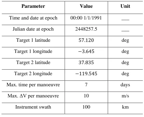
Table 1. Constants.

Parameter Value Unit

Gravitational Parameter 3.986 × 1014 m3/s2

Mean radius of Earth 6371 km

Coefficient of J2 for Earth 0.0010827 ___

Angular velocity of Earth 7.29212 × 10−5 rad/s

Table 2. Mission Parameters.

Parameter Value Unit

Time and date at epoch 00:00 1/1/1991 ___

Julian date at epoch 2448257.5 ___

Target 1 latitude 57.120 deg

Target 1 longitude −3.645 deg

Target 2 latitude 37.835 deg

Target 2 longitude −119.545 deg

Max. time per manoeuvre 7 days

Max. ΔV per manoeuvre 10 m/s

Instrument swath 100 km

Figure 4: Map highlighting both flyover targets.

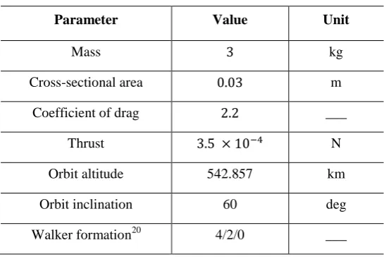
Table 3. Spacecraft parameters.

Parameter Value Unit

Mass 3 kg

Cross-sectional area 0.03 m

Coefficient of drag 2.2 ___

Thrust 3.5 × 10−4 N

Orbit altitude 542.857 km

Orbit inclination 60 deg

Walker formation20 4/2/0 ___

Analysing all the possible manoeuvres to complete the proposed mission produces a graph of 10726 nodes, where each node represents the system state immediately after a target flyo-ver. One node (Node 0) represents the initial system state at epoch. This Node 0 is connected to 119 nodes that represent the system state after flyover of one target (i.e. Stage 1). These 119 nodes, in turn, are connected to 10606 nodes (i.e. Stage 2). Of these, 6157 nodes repre-sent the system state after a satellite subsequently flies over the second target (i.e. sequential manoeuvres), and 4449 nodes are at the end of transplanted edges, representing the case in which both spacecraft manoeuvre in tandem to flyover both targets (i.e. simultaneous ma-noeuvres). Generating this full graph of results takes approximately 80 minutes on a desktop computer running Windows 7 with 8 GB of RAM.

RESULTS FOR FULL GRAPH

Dijkstra’s algorithm can provide a shortest path solution when the graph is weighted and the path must terminate at a Stage 2 node (i.e. the path must flyover both targets). However, the real strength of taking a graph approach is in identifying the routes and options through the graph.

Minimum Time Solution

For the case presented, Dijkstra’s algorithm identified the shortest path as taking 2 days 14 hours and 11 minutes and requiring 7.037 m/s ΔV. Contrary to what may be expected, this is a sequential manoeuvre; intuitively, it would seem more efficient to move two satellites simul-taneously but the best possibility using such an approach is one minute slower than the short-est sequential manoeuvre path. Using a shortshort-est path algorithm to analyse the graph provides very limited information about the overall scenario and the manoeuvre possibilities within it. However, by restricting the graph to consider only manoeuvres with times close to the mini-mum, alternative options can be identified and considered. These may, for example, require less ΔV than the absolute minimum time solution, or may have more redundant options avail-able at Stage 2 of the scenario.

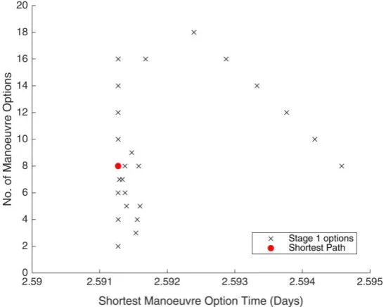
Consider, for example, the same graph but in this case the edges from Stage 1 to Stage 2 are only included if the path length from source through to Stage 2 is less than 10 m/s ΔV in total, and both target flyovers are completed within 5 minutes of the time taken by the shortest path. The shortest path remains the same (2 days 14 hours and 11 minutes), as the ΔV re-quired is only 7.037 m/s. With the constraints of this graph, after the first manoeuvre of the shortest path, there exist 8 feasible manoeuvres (4 sequential and 4 simultaneous) for reaching the second flyover. However, other paths exist that take only slightly longer but present more manoeuvre options, as displayed in Figure 5. In particular, there is a path that takes 1 second longer than the shortest path but has 16 manoeuvre options (8 sequential and 8 simultaneous) that conform to the 10 m/s ΔV and 5-minute time constraints. The graph analysis presents these options to the operators allowing them to make informed trade-offs. The decision is be-tween selecting the shortest path route or a path that takes slightly longer but provides more redundant manoeuvre options. Given how short the time difference is in this case, the deci-sion of selecting the path with more options seems obvious as it provides flexibility in dealing with uncertainty in the manoeuvre execution. It can also identify high performing simultane-ous manoeuvres that could be used in conjunction with a sequential manoeuvre to add redun-dancy in covering a target. Of note is that also seen in Figure 5 is a Stage 1 node with eight-een options. This choice is less attractive as all eighteight-een of these options are simultaneous manoeuvres and, therefore, these options provide no added flexibility to accommodate errors in manoeuvre execution. This emphasises the need to understand the range of operational scenarios possible, rather than selecting the fastest path, or that with the most options, without further investigation.

Minimum ΔV Solution

If the ΔV constraint is expanded to include paths with a total ΔV of 5 m/s plus drag com-pensation, then a slightly superior number of options are available from a Stage 1 node not on the shortest path as shown in Figure 6. However, all 9 of the options available are simultane-ous manoeuvres, whereas the 8 options available to the Stage 1 node on the shortest path are evenly split between sequential and simultaneous manoeuvres.

Figure 5: Comparison of options, from Stage 1 nodes, that complete both target flyovers within 5 minutes of the fastest flyover completion time.

RESULTS FOR REDUCED GRAPH

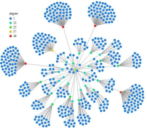
This analysis is done using the same graph as in the Results Section above, but here the graph is reduced to consider only two satellites, one in each orbit plane. It also only considers solutions that would be in view for a system with a swath width of 50 km, as opposed to the previously defined 100 km, and only includes manoeuvres requiring up to 5 m/s ΔV plus that required for drag compensation. This will demonstrate how the proposed method can be used for efficient mission design by enabling the effect of changes in mission parameters to be rap-idly assessed by retraversing the graph, without the need to recalculate individual manoeuvre options. The reduced graph contains 510 nodes, with 1 source node, 29 Stage 1 nodes, 240 Stage 2 nodes at the end of sequential manoeuvres and 240 that were the product of simulta-neous manoeuvres. This is shown in Figure 7.

Minimum Time Solution

The constraints on the ΔV to be used for each manoeuvre and the narrow swath width pro-duces a smaller, more constrained, graph. Despite these changes, the shortest path remains similar, taking 2 days 14 hours and 13 minutes. However, in this case it is a simultaneous ma-noeuvre that requires significantly more ΔV than in the full graph case, requiring 9.04 m/s. The shortest time sequential manoeuvre takes 2 days 23 hours and 53 minutes and also re-quires a ΔV of 9.04 m/s.

When then applying the restriction, from the full graph analysis, that paths cannot take more than 5 minutes longer than the shortest path, there are two possible paths from the Stage 1 node of the shortest path. These paths are both simultaneous manoeuvres; in fact, the 5-minute time window would need to be extended to almost ten hours before any alternative sequential paths were eligible.

Minimum ΔV Solution

compared with the 2.045 m/s ΔV possible in the full graph, due to the reduced swath width and fewer satellites. As in the full graph, the shortest path is also in possession of a compara-tively large number of options from the Stage 1 node to the Stage 2 node; four 4 m/s ΔV ma-noeuvres in this case.

CONCLUSION & FUTURE WORK

The method of analysing responsive spacecraft manoeuvres using graph techniques allows designers and operators to consider the full responsive mission and make informed choices considering the entire operational scenario, rather than just an individual manoeuvre. This can result in more efficient operations by avoiding manoeuvres that may seem appealing but lead to inefficient subsequent options. The graph captures not only the best combination of ma-noeuvres but can also highlight whether an initial manoeuvre is the start of a path with only one option or a multitude of them. Identifying manoeuvres that produce more options later in the mission is a useful insight for operators. It can reduce the chance that errors in the execu-tion of a manoeuvre would prevent a target from being seen or it can allow an operator to have a contingency plan, including tasking multiple flyovers of the same target. The use of the graph can also provide insights by highlighting non-intuitive solutions, for example, that it may be faster for one satellite to perform two targeting manoeuvres than for two satellites to manoeuvre simultaneously. The presented technique, therefore, provides a scalable method of analysing the performance of responsive constellations in long-term operational scenarios, without the need to apply restrictions or assumptions to the problem prior to analysis.

A key area for future work will be to include uncertainty in the analysis, so that competing options can be assessed in terms of their resilience to change. This will allow for scenarios with uncertain future needs to be considered. Considering a broader range of case studies with a greater number of targets and spacecraft, and varying mission parameters will allow for fa-vourable spacecraft and constellation architectures to be identified. Additionally, the applica-tion of more complex graph theoretical techniques will allow for more interesting insights into the challenge of responsive spacecraft operations.

REFERENCES

[1] Voigt, S., Giulio-Tonolo, F., Lyons, J., Kučera, J., Jones, B., Schneiderhan, T., Platzeck, G., Kaku, K., Hazarika, M.K., Czaran, L. and Li, S., “Global trends in satellite-based emergency mapping,” Science, Vol. 353, Issue 6296, 2016, pp. 247-252. doi: 10.1126/science.aad8728

[2] Santilli, G., Vendittozzi, C., Cappelletti, C., Battistini, S. and Gessini, P., “CubeSat constellations for disaster management in remote areas,” Acta Astronautica, Vol. 145, pp. 11-17. doi: 10.1016/j.actaastro.2017.12.050

[3] Gopinath, G., “Free data and Open Source Concept for Near Real Time Monitoring of Vegetation Health of Northern Kerala, India,” Aquatic Procedia, Vol. 4, 2015, pp. 1461-1468. doi: 10.1016/j.aqpro.2015.02.189

[4] Boshuizen, C., Mason, J., Klupar, P. and Spanhake, S., “Results from the planet labs flock constel-lation,” Presented at the AIAA/USU Small Satellite Conference, 2014.

[5] Platzer, P., Wake, C., and Gould, L., “Smaller Satellites, Smarter Forecasts: GPS-RO Goes Main-stream,” Presented at the AIAA/USU Small Satellite Conference, 2015.

[7] Morin, J., “Four steps to global management of space traffic,” Nature, Vol. 567, 2019, pp. 25-27. doi: 10.1038/d41586-019-00732-7

[8] Skinner, M.A., Jah, M.K., McKnight, D., Howard, D., Murakami, D. and Schrogl, K.U., “Results of the international association for the advancement of space safety space traffic management working group,” Journal of Space Safety Engineering, In Press, 2019. doi: 10.1016/j.jsse.2019.05.002

[9] McGrath, C.N., and Macdonald, M., “General Perturbation Method for Satellite Constellation Re-configuration using Low-Thrust Maneuvers,” Journal of Guidance, Control and Dynamics, In Press, 2019. doi: 10.2514/1.G003739

[10]McGrath, C.N., “Analytical Methods for Satellite Constellation Reconfiguration and Reconnais-sance using Low-Thrust Manoeuvres,” PhD, Mechanical and Aerospace Engineering, University of Strathclyde, 2018.

[11]Bate, R.R., Mueller, D.D. and White, J.E., Fundamentals of Astrodynamics, Dover, New York, 1971, pp. 58-60.

[12]E. W. Dijkstra, "A note on two problems in connexion with graphs," Numerische mathematik, vol. 1, pp. 269-271, 1959.

[13]Carver, S., Comber, L., Fritz, S., McMorran, R., Taylor, S., and Washtell, J., "Wildness study in the Cairngorms National Park," Technical report, University of Leeds, 2008.

[14]Gray, A., and Levy, P., "A review of carbon flux research in UK peatlands in relation to fire and the Cairngorms National Park," Technical report, Natural Environment Research Council Centre for Ecology & Hydrology, July 2009.

[15]"National Park Service visitor use statistics for Yosemite National Park," https://irma.nps.gov/Stats/Reports/Park/YOSE, 2017. Accessed: 09/02/2018.

[16]Lutz, J. A., Van Wagtendonk, J. W., Thode, A. E., Miller, J. D., and Franklin, J. F., "Climate, lightning ignitions, and fire severity in Yosemite National Park, California, USA," International Journal of Wildland Fire, Vol. 18, No. 7, 2009, pp. 765-774. doi:10.1071/WF08117.

[17]Kane, V. R., North, M. P., Lutz, J. A., Churchill, D. J., Roberts, S. L., Smith, D. F., McGaughey, R. J., Kane, J. T., and Brooks, M. L., "Assessing fire effects on forest spatial structure using a fu-sion of Landsat and airborne LiDAR data in Yosemite National Park," Remote Sensing of Envi-ronment, Vol. 151, 2014, pp. 89-101. doi: 10.1016/j.rse.2013.07.041.

[18]Krejci, D., Mier-Hicks, F., Thomas, R., Haag, T. and Lozano, P., “Emission characteristics of pas-sively fed electrospray microthrusters with propellant reservoirs,” Journal of Spacecraft and Rock-ets, Vol. 54, No. 2, 2017, pp.447-458. doi: 10.2514/1.A33531

[19]Mier-Hicks, F. and Lozano, P.C., “Electrospray Thrusters as Precise Attitude Control Actuators for Small Satellites,” Journal of Guidance, Control, and Dynamics, Vol. 40, No. 3, 2017, pp. 642-649. doi:10.2514/1.G000736