Single polymer chains

pg. 35 Tapping mode imaging avoids frictional forces and minimises adhesional forces; it is the preferred method for imaging soft samples.

Single P o ly m e r C h a in s

B e lin d a J ea n H au p t

A thesis submitted for the degree of

Doctor of Philosophy of the Australian National University

Research School of Chemistry

Institute of Advanced Studies

This thesis is an account of research carried out at the Research School of Chem­ istry, Australian National University for the degree of Doctor of Philosophy.

Although the material presented herein is primarily my own independent re­ search, several collaborators should be acknowledged for their contributions. The atomic force microscopy (AFM) experiments presented in Chapter 4 were performed with the help of Dr Tim Senden and Anthony Hyde is also thanked for his assistance in the design and construction of the inverted dewar used in these experiments. We thank Horst Neumann for his assistance with the synthesis of PNIPAM and in its characterization, Jelica Strauch at the Key Centre for Polymer Colloids, the Univer­ sity of Sydney for the GPC analysis of PNIPAM, used in AFM studies in Chapter 4. Dr David Williams contributed to the development of the simulation program used for generating the results presented in Chapter 6.

The work described in this thesis is original and has not previously been submit­ ted for a degree or diploma in any other University or College.

iii

A ck n o w le d g em en t s

There are many people whose assistance, guidance and friendship have not only made this thesis possible but my time at the A.N.U. memorable. I would specifically like to thank the following people for their invaluable contributions:

Firstly, my supervisor Dr. Edie Sevick, for her enthusiasm for science, insistence on overseas conferences, and her obsession with regular exercise (the result of which I am now a dedicated gym junkie). My temporary supervisor, Prof. David Williams, of the Department of Applied Mathematics, for his very, non-politically correct sense of humour and providing invaluable assistance with my research while Edie was away having their son, Max. I’d also like to thank Dr. Tim Senden, for his generous support with my experiments at the Department of Applied Mathematics and for introducing me to liquorice flavoured espressos.

Prof. Denis Evans, the Dean of the Research School of Chemistry, who gave me a real sense of hope in the future of science in Australia. Dr. Ray Withers, Graduate Convenor of the RSC and avid bush poetry fan, who together with Prof. Evans and the rest of the P&T group have made for some pretty interesting Morning and Afternoon Teas.

To the many people at the Research School of Chemistry and Department of Applied Mathematics, who made them enjoyable places to work. An incomplete list of names: Joanne Harvey, Keith Porter, Ken McRae, Leonie Chow, David Loong and Lasse Noren from the RSC and Ian Miller, Ira Cooke, Tristram Alexander, Chiara Neto, Vince Craig, Janey Wood, and Scott Miller from the Research School of Physical Sciences and Engineering.

To the computing staff for their invaluable support. Horst Neumann, from the RSC for his help with my one and only synthesis and Anthony Hyde, from the Department of Applied Mathematics, for his help in the necessary modifications to the instrument used in my experiments.

My friends here: Louise Sutherland, Doug Aberdeen, Cathie Menon, Tanya McKay, Bina D’Costa, and Wayne Solomon; and interstate/OS: Jennifer Clancy, Thuy Ho, Michael and Chris Noney, Jason Sky, David Carberry, Gemma Drew, Nikolai Tolich, Debbie Watson, Kevin Fleming, Freya Mearns and Felix Ho; who have been a great source of sanity, inspiration and fun.

A b s tr a c t

Atomic Force Microscopy has been used to investigate the detachment of single polymer chains from surfaces and to measure the picoNewton forces required to extend the chain orthogonal to the surface. Such recent experiments show that the force-extension profiles provide interesting signatures which might be related to the progressive detachment of the chain from a surface.

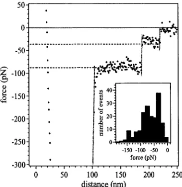
We present experimental evidence of the Rayleigh instability of a single chain in poor solvent conditions using single molecule force microscopy. Poly-N-isopropyl- acrylamide (PNIPAM) and polyethylene oxide (PEO) are adsorbed onto silicon ni­ tride surfaces in various solutions corresponding to poor and good solvent conditions. In good solvent conditions, the force-separation profile is identical to that described previously and attributed to the elastic stretching of single polymer chains. However, in poor solvent conditions, we see a dramatically different force profile, characterised by steps or plateaus of constant force. These plateaus signature the pull-out” of chain segments from collapsed globules of polymer collected at each of the sepa­ rating surfaces. A statistical analysis of the large number of force profiles collected indicates that these plateaus are stepped or quantised, suggesting pull-out of several chains of different length. Moreover, the frequency of the steps shows an interesting pattern which distinguishes pulled loops from pulled tails.

We also investigate theoretically the detachment of a single polymer chain from a weakly adsorbing surface. Using equilibrium scaling analysis and activation kinetics, we predict force versus extension profiles for various extension rates. The qualitative features that we predict, such as saw-tooth force-profiles with detachment forces which decrease with extension, maximal yielding forces at high extension rates, and featureless force profiles at large extension, are also seen in experiment.

C o n te n ts

1 In tr o d u c tio n 1

1.1 Introduction... 1

1.2 Aims and Thesis O u tlin e ... 3

References... 5

2 B a ck g ro u n d and M eth o d o lo g y : T ools u sed in th is T h e sis 11 2.1 Polymer Chain M o d e ls... 11

2.1.1 Freely Jointed Chain M o d e l... 12

2.1.2 The Gaussian Chain and the Bead-Spring Model ... 14

2.2 Thermodynamics and the Polymer S y s te m ... 15

2.2.1 Stretching a Polymer C h a i n ... 15

2.2.2 Polymer Confinement... 18

2.2.3 Polymer Solvent T y p e s ...20

2.3 Simulation M ethods... 22

2.3.1 Molecular D y n a m ic s ...22

2.3.2 Langevin D ynam ics...23

2.3.3 Radius of G y ra tio n ...25

2.4 Summary ... 25

References... 27

3 A to m ic F orce M icro sco p e: T h e In str u m e n t an d Its U s e 29 3.1 Introduction to the Atomic Force Microscope... 29

3.2 Cantilever and Probe T i p s ...31

3.2.1 Spring Constant C alib ratio n ... 32

3.3 Laser Beam Deflection S e n s o r ...34

3.4 Piezoelectric Scanners ...34

3.4.1 Piezo-element C a lib ra tio n ... 35

3.5 Modes of O peration... 35

3.6 Force versus Distance Curves ...36

3.7 Sample P rep aratio n ... 38

References... 41

4 A F M E v id e n c e o f th e R a y le ig h I n s ta b ility in S in g le P o ly m e r C h a in s 45 4.1 Introduction... 45

4.2 Experimental S ectio n ... 51

4.2.1 Materials ... 51

4.2.2 Equipment and T ech n iq u e... 51

4.3 Force profiles of PNIPAM ...53

4.4 Force profiles of P E O ... 59

4.5 D iscussion... 67

References... 73

5 T h e D e ta c h m e n t o f a P o ly m e r C hain from a W ea k ly A d so rb in g Su rface u sin g an A F M T ip 75 5.1 Introduction... 75

5.2 Slow Extension of a Weakly-Adsorbed C h a in ... 77

5.3 Intermediate Extension Rates of a Weakly-Adsorbed C h a in ...78

5.3.1 Multiple detachments from a homogeneous surface... 79

5.4 Fast extension of an adsorbed c h a in ...82

5.5 Conclusion... 85

5.5.1 Work Since Publication...85

References... 87

6 T h e effect o f ra tes on th e force profiles for r ip p in g -o ff a sin g le p o ly ­ m er ch a in from a surface: A L a n g ev in S im u la tio n S tu d y 89 6.1 Introduction... 89

6.2 Model for S im u latio n ... 90

6.3 Initialisation and Equilibration ...92

6.4 Pulling ”Experiments” ... 97

6.4.1 Continuous Pulling Mode in the z-direction ...97

6.4.2 Tem perature... 102

6.4.3 Different Rates of Retraction ...104

6.4.4 A Different Mode of Pulling: Oscillating T i p ... 104

6.5 Constant F o r c e ...108

6.6 D iscussion...I l l References... 118

L ist of F ig u re s

2.1 The freely jointed chain m o d el... 12

2.2 The beads-spring m o d e l ... 14

2.3 Theoretical force profiles of different m o d e l s ... 18

2.4 An ideal chain trapped between two walls ... 19

3.1 Schematic diagram of an atomic force microscope (A F M )... 30

3.2 A schematic of the extension of an end-tethered chain using an AFM p ro b e...31

3.3 An example of the plots used to determine the spring constant of the cantilever for an AFM experim ent...33

3.4 A schematic of the silicon calibration grating model TG Z03... 36

3.5 A typical force curve for Milli-Q pure water ...37

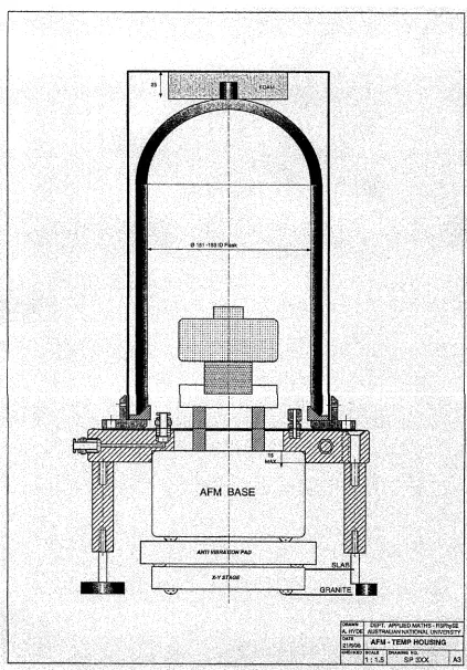
3.6 A schematic diagram of the inverted vacuum d e w a r ... 39

3.7 The calibration graph for the th e r m is to r ... 40

4.1 The theoretically predicted (a) free energy profile and (b) force profile 47 4.2 The van der Waals isotherm (a) and the theoretically predicted force pr ofile ( b ) ... 48

4.3 Schematic of the Rayleigh instability for a single polymer chain in a poor so lv e n t... 50

4.4 The reaction scheme (a) and the 13C n.m.r. spectra of PNIPAM (b) . 52 4.5 Force profiles for PNIPAM in aqueous solution in (a) good and (b) poor solvent conditions... 54

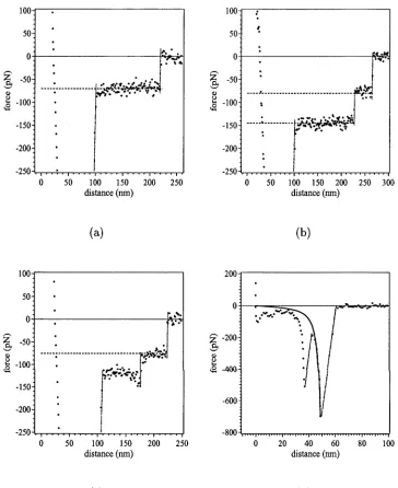
4.6 Representative force profiles for PNIPAM in aqueous solutions in poor solvent conditions... 55

4.7 Histograms summarising the statistics of force events for PNIPAM . . 56

4.8 AFM images of PN IPA M ... 57

4.9 Force profiles and histogram summarising the set of profiles for PEO in 0.45M K2SO4... 61

4.10 Representative force profiles for PEO in 0.45M K2SO4... 62

4.12 Representative force profiles for PEO in aqueous no-salt solution . . . 64 4.13 A force profile and histogram for PEO in aqueous 0.25 M KNO3 solution 65 4.14 Representative force profiles for PEO in aqueous 0.25 M KNO3 solution 66 5.1 Schematic illustration of the “grabbing” and pulling of a loop . . . . 76 5.2 Scaled force profile for the detachment of an adsorbed chain of

equi-sized lo o p s... 81 5.3 Force profiles at different extension r a t e s ... 82 5.4 Force profile for the detachment of a chain having unequal loops . . . 83 5.5 The number of instantaneous detachments versus the scaled extension

rate ...84 6.1 (a) The FENE spring force, f spring(i/kßT, versus the monomer-monomer

bond length, l/a and (b) the surface force, f surf a / k ß T, versus z- distance, z/ a ... 91 6.2 The initial configuration of a chain of length N — 20 93 6.3 Radius of gyration squared, < >, versus number of timesteps . . . 94 6.4 The z-height of an adsorbed chain, Zheight/a, versus number of timesteps

at (a) e = 0.1 and (b) e — 0 .0 1 ...96 6.5 (a) The average z-height, zavg/ a, versus chain size, N/ a and (b) The

average z-height, zavg/a, versus the te m p e ra tu re ... 96 6.6 A pulling ’’experiment” ...98 6.7 (a) Fraction of ’’adsorbed” monomers versus timesteps, (b) force,

f a / k ß T , versus displacement, z/a, profile and (c) spring force, f springt/kßT, versus bond number in chain, j at e = 4 0 .0 ... 100 6.8 (a) Fraction of ’’adsorbed” monomers versus timesteps, (b) force,

f a / k ß T, versus displacement, z/a, profile and (c) spring force, f springa/ k ß T , versus bond number in chain, j at e = 0.1 ... 101 6.9 (a) Histogram of the detachment forces, fdet^/kßT, of monomers in

a chain of length N = 50, £ = 40.0 at different temperatures and force, f a / k ß T, versus displacement, z / a, profiles at (b) kßTn = 1.0, (c) kßTn — 0.1 and (d) kßTn — 0 .0 1 ... 103 6.10 Force, f a / k ß T, versus displacement, z / a, profiles at different pulling

rates (a) v = 1/mi/s, (b) v = 10/mi/s and (c) v = 100^zm /s... 105 6.11 (a) Displacement, z / a, versus timesteps plot, (b) force, f a / k ß T, ver­

sus timesteps profile and (c) fraction o f ’’adsorbed” monomers versus timesteps graph for an oscillatory pulling e x p e rim e n t...107 6.12 Spring force, f springt/kßT, versus the bond number in the chain, j,

LIST OF FIGURES ix

6.13 The z-displacement of the first monomer in the chain, 2/a, versus

L ist o f T ab les

6.1 The < R* >for N = 50 at k BT = 0.1... 112

6.2 The < Ry >for N = 100 at k ß T = 0.1...113

6.3 The < T&g >for N = 200 a t k BT = 0.1... 114

6.4 The < K* >for N = 50 at k BT = 1.0... 115

C hapter 1

In trod u ction

1.1

Introduction

A polymer chain consists of a large number of identical chemical units which are referred to as monomers. The simplest polymer is polyethylene and consists of the chemical unit of (-CH-2 — C H2—). The total number of monomers in a chain is represented by N and is referred to as the degree of polymerisation. Polymers can be linear, branched or have ring configurations. Those that consist of only the one type of chemical unit are known as homopolymers. Alternatively, polymers can also consist of different monomers which can be in a random or regular sequence and are known as copolymers. Heteropolymers consist of several different types of monomers which occur in a non-regular pattern and are commonly found in biopolymers e.g., nucleic acids, polysaccharides and proteins. Monomeric units may also be neutral or charged, those that carry a charge are called polyelectrolytes.

Polymer chains are large molecules, especially when compared to surrounding solvent molecules. In polymer liquids, any given polymer chain only experiences an average of its surrounding due to its many degrees of freedom and its ability to interact with its neighbours. Therefore only mean properties of an individual chain need to be determined. Macroscopic behaviour of polymer solutions are largely determined by the size of the chain. Due to this dependence, then if a few molecular sized parameters are equivalent, then different systems will behave the same. Hence, we consider polymer chains in terms of their molecular size and as being spaghetti­ like.

Previously, the behaviour of polymers could only be studied using bulk methods which were limited in that they could only measure macroscopic ensemble averages and could not measure the elastic properties of polymers directly, relying on the­ oretical models. However, the development of new experimental techniques such as Atomic Force Microscopy (AFM) 1-30 and optical/magnetic tweezers31-39 have

in recent years. These new techniques now make it possible to manipulate single polymer chains by imposing nanometer scale deformations and measuring forces on the scale of picoNewtons. Theoretical studies of perturbing a chain have also been conducted, the majority of these use models that are not atomistic, as the properties of interest are of the molecular scale. These compliment experimental studies, providing insight into experimentally obtained results and make predictions for experiments not yet conducted.

Single polymer chains are of interest to a wide variety of fields including bio­ physics, colloidal stabilisation, lubrication and adhesion. 1 -9 ,31,32,40,41 The bioploymer

DNA has been widely studied, this is due to its importance in biological processes, as it is important in transcription, replication and packaging into chromosomes.33-35,42

An understanding of the physics of molecular interactions would therefore provide insight not only in biological interactions, but would be of use in the development of materials for specific industrial purposes and macroscopic properties.

We use the AFM to study the behaviour of synthetic polymer chains in differ­ ent solvent conditions. Specifically, we study the stretching behaviour of adsorbed, single polymer chains in poor solvent. Over recent years, an ever increasing number of polymer systems, both biological and synthetic have been studied using both the AFM and optical tweezers, typically in good solvent conditions. Most notably, are the studies on the biopolymers DNA3 ,10,32-30,38 and titin (the giant globular mus­

cle protein) , 27,36,39 which have been manipulated using both the AFM and optical

tweezers and their mechanical properties determined. Some experimental studies measure the force required to detach a chain from an adsorbing surface and in many of these, the force versus extension profile exhibits sharp discontinuities wdiich have been interpreted in terms of unadsorbed loops of the chain. A number of different single-chain systems have been studied using the AFM and include both synthetic polymers7 -9 ,1 1 ,1 3 ,16-25,29,30 and biopolymer chains.4 ,10,12,14,26-28 From these studies,

the adhesion and elasticity of individual polymer chains have been measured, also, and the structure and the unfolding/folding behaviour of individual domains in biopolymers been investigated.

We have also used scaling analysis, a theoretical treatment developed by de- Gennes43 and discussed in greater detail in the following chapter, to investigate the

physical behaviour of single polymer chains as they are detached from an adsorbing surface. The physics of polymers have been the studied since the synthesis of these molecules and most notably by deGennes, Flory, Doi, Edwards and Kuhn.43-47 Of

the numerous theoretical studies of polymer chains, there have been several that have investigated the stretching behaviour of a single polymer chain in solution un­ der various solvent conditions.43-53 The behaviour of a polymer chain adsorbed to a

1.2. A im s and T h e sis O u tlin e 3

However, the compression with finite sized objects54-58 has only recently been stud­

ied and is due to the advent and use of the AFM to probe surface bound chains. Similarly, theoretical treatments of AFM single chain experiments, where the sur­ face adsorbed chains are extended have also recently received attention. The stud­ ies conducted have intended to explain experimentally obtained results for different polymer systems as well as make predictions for features observed in force extension curves.9,18,59-62

Simulation has also been used to study both the static and dynamic properties of single polymer chain under tension in this thesis. A number of different simulation techniques have been used to study the behaviour of a chain in solution, many of which confirm the results of theoretical studies.63-69 The compression of polymer

chains adsorbed or grafted to a surface has also been studied, where conformational transitions are found to occur when the object compressing the chain is of finite size e.g., an AFM probe.70-74 The stretching of surface bound chains orthogonal

and perpendicular to a surface have also been investigated using simulation tech­ niques. 75-78 These simulations were used to study the dynamics of the chains as

they were extended and in some instances, detached from the surface.

The theme of this thesis has been the manipulation of single polymer chains using the atomic force microscope. In this thesis, we have combined theory with simulation and experiments to investigate the detachment of single polymer chains adsorbed to a surface.

1.2

A im s an d T h e sis O u tlin e

Specifically, our aim has been to investigate the dynamics and physics of de­ taching a single polymer chain from an adsorbing surface using the AFM. In this thesis, we have used scaling analysis and activation kinetics to make predictions for the force profiles of single chain experiments using the AFM. We investigate how the detachment process and features observed in force versus extension profiles vary, depending on the rate of detachment of the chain. Following on from this is a study of the dynamics of single chain AFM experiments. Using simulation we are able to study the effect of a number of system parameters quite easily that would otherwise be quite difficult to do experimentally. The effect of varying the solvent quality on the force profile has also been investigated experimentally using a modified AFM. We have studied several different aqueous polymer systems in order to determine if differences in the force profiles for single chain experiments are attributable to the solvent conditions and not a specific polymer system.

REFERENCES 5

R eferen ces

[1] Baumgartner, W.; Hinterdorfer, R; Ness, W.; Raab, A.; Vestweber, D.; Schindler, H.; Drenckhahn, D. Proceedings of the National Academy of Sciences

of the United States of America 2000, 97, 4005.

[2] Florin, E.-L.; Moy, V. T.; Gaub, H. E. Science 1994, 264, 415.

[3] Zlatanova, J.; Lindsay, S. M.; Leuba, S. H. Progress in Biophysics and Molecular Biology 2000, 74, 37.

[4] Oesterhelt, F.; Oesterhelt, D.; Pfeiffer, M.; Engel, A.; Gaub, H. E.; Müller, D. J. Science 2000, 288, 143.

[5] Müller, D. J.; Baumeister, W.; Engel, A. Proceedings o f the National Academy of Sciences of the United States of America 1999, 96, 13170.

[6] Camesano, T. A.; Logan, B. E. Environmental Science and Technology 2000. 34, 3354.

[7] Bemis, J. E.; Akhremitchev, B. B.; Walker, G. C. Langmuir 1999, 15, 2799. [8] Courvoisier, A.; Isel, F.; Frangois, J.; Maaloum, M. Langmuir 1998, 14, 3727. [9] Hügel, T.; Grosholz, M.; Clausen-Schaumann, H.; Pfau, A.; Gaub, H. ; Seitz,

M. Macromolecules 2001, 34, 1039.

[10] Strunz, T.; Oroszlan, K.; Schäfer, R.; H.-J. Güntherodt, H. -J. Proc. Natl. Acad. Sei. USA 1999, 96, 11277.

[11] Ortiz, C.; Hadziioannou, G. Macromolecules 1999, 32, 780.

[12] Marszalek, P. E.; Oberhäuser, A. F.; Pang, Y. -P.; Fernandez, J. M. Nature 1998, 396, 661.

[13] Senden, T. J.; di Meglio, J. -M.; Auroy, P. Eur. Phys. J. B 1998, 3, 211. [14] Rief, M.; Oesterhelt, M. F.; Hcymann, B.; Gaub, H. E. Science 1997, 275,

[15] Bustamante, C.; Marko, J. F.; Siggia, E. D.; Smith, S. Science 1994, 265, 1599. [16] Oesterhclt, F.; Rief, M.; Gaub, H. E. New Journal of Physics 1999. 1, 6.1. [17] Zhang, W.; Zou, S.; Wang; C.; Zhang, X. J. Phys. Chem. B 2000, 104, 10258. [18] Chätellier, X.; Senden, T. J.; Joanny, J. -F.; di Meglio, J. -M. Europhysics

Letters 1998, 4U 303.

[19] Kikuchi, H.; Yokoyama, N.; Kajiyama, T. Chemistry Letters 1997, 11, 1107. [20] Maaloum, M.; Courvoisier, A. Macromolecules 1999, 32, 4989.

[21] Li, H.; Liu, B.; Zhang, X.; Gao, C.; Shen, J.; Zou, G. Langmuir 1999, 15, 2120. [22] Li, H.; Zhang, W.; Xu, W.; Zhang, X. Macrom,olecules 2000, 33, 465.

[23] Al-Maawali, S.; Bemis, J. E.; Akhremitchev, B. B.; Leecharoen, R.; Janesko, B. G.; Walker, G. C. J. Phys. Chem. 2001, 105, 3965.

[24] Gamier, L.; Gauthier-Manuel, B.; van der Vegte, E. W.; Snijders, J.; Hadzi- ioannou, G. Journal of Chemical Physics 2000, 113, 2497.

[25] Yamamoto, S.; Tsujii, Y.; Fukuda, T. Macromolecules 2000, 33, 5995.

[26] Li, LL; Rief, M.; Oesterhelt, F.; Gaub, H. E. Advanced Materials 1998, 3, 316. [27] Rief, M.; Gautel, M.; Oesterhelt, F.; Fernandez, J. M.; Gaub, H.E. Science

1997, 276, 1109.

[28] Carrion-Vazquez, M.; Oberhäuser, A. F.; Fowler, S. B.; Marszalek, P. E.; Broedel, S. E.; Clarke, J.; Fernandez, J. M. Proc. Natl. Acad. Sei. USA 1999, 96, 3694.

[29] Senden, T. J. Current Opinion in Colloid and Interface Science 2001, 6, 95. [30] Merkel, R. Physics Reports 2001, 346, 343.

[31] Carl, P.; Kwok, C. H.; Manderson, G.; Speicher, D. W.; Discher, D. E. Pro­ ceedings of the National Academy of Sciences of the Ujiited States of America

2001, 98, 1565.

[32] Shivashankar, G. V.; Feingold, M.; Krichcvsky, O.; Libchaber, A. Proceedings of the National Academy of Sciences of the United States of America 1999, 96, 7916.

R E F E R E N C E S 7

[34] Cui, Y.; Bustamante, C. Proceedings of the National Academy of Sciences of the United States of America 2000. 97, 127.

[35] Bennink, M. L.; Leuba, S. H.; Leno, G. H.; Zlatnova, J.; de Grooth, B. G.; Greve, J. Nature Structural Biology 2001, 8, 606.

[36] Tskhovrebova, L.; Trinick, J.; Sleep, A.; Simmons, R. M. Nature 1997, 387, 308.

[37] Smith, S. B.; Cui, Y.; Bustamante, C. Science 1996, 271, 795. [38] Strick, T. R.; Croquette, V.; Bensimon, D. Nature 20 0 0, fOf, 901.

[39] Kellermayer, M. S. Z.; Smith, S. B.; Granzier, H. L.; Bustamante, C. Science 1997 , 276, 1112.

[40] Krammer, A.; Lu, H.; Israelwitz, B.; Schulten, K.; Vogel, V. Proceedings of the National Academy of Sciences of the United States of America 1999, 96, 1351.

[41] Lasic, D. D. Liposomes: from Physics to Applications; Elsevier: Amsterdam and New York, 1993.

[42] Hansma, H. G.; Browne, K. A.; Bezanilla, M.; Bruice, T. C. Biochemistry 1994, 33, 8436.

[43] de Gennes, P. -G. Scaling Concepts in Polymer Physics; Cornell University Press: Ithaca, 197 9.

[44] Doi, M.; Edwards, S. F. The Theory of Polymer Dynamics; Oxford University Press: Oxford, 1986.

[45] Flory, P. J. Principles of Polymer Chemistry; Cornell University Press: Ithaca, 1992.

[46] Flory, P. J. Statistical Mechanics of Chain Molecules; Hanser Publishers: New York, 1989.

[47] Evans, D. F.; Wennerström, H. The Colloidal Domain: Where Physics, Chem­ istry and Biology Meet, 2nd. ed.; Wiley-VCH: New York, 1999.

[48] de Gennes, P. G. Macromolecules 1976, 9, 587. [49] Pincus, P. Macromolecules 1976, 9, 386.

[52] Marko, J. F. Physical Review E 1998, 57, 2134.

[53] Sarkar, A.; Leger, J.-F.; Chatcnay, D.; Marko, J. F. Physical Review E 2001, 63, 051903-1.

[54] Subramanian, G.; Williams, S. R. M.; Pincus, P. A. Macromolecules 1996, 29, 4045.

[55] Guffond, M. C.; Williams, D. R. M.; Sevick, E. M. Langmuir 1997, 13, 5691. [56] Ennis, J.; Sevick, E. M.; Williams, D. R. M. Physical Review E 1999, 60, 6906. [57] Sevick, E. M. Macromolecules 2000, 33, 5743.

[58] Ennis, J.; Sevick, E. M. Macromolecules 2001, 34, 1908.

[59] Chätellier, X.; Joanny, J.-F., Physical Review E 1998, 57, 6923.

[60] Lubensky, D. K.; Nelson, D. R., Physical Review Letters 2000. 85, 1572. [61] Tamashiro, M. N.; Schiessel, H., Macromolecules 2000, 33, 5263.

[62] Zhulina, E.; Walker, G. C.; Balazs, A. C., Langmuir 1998, 14, 4615. [63] Hatfield, J. W.; Quake, S. R. Physical Review Letters 1999, 82, 3548. [64] Kreitmeier, S.; Wittkop, M.; Göritz, D. Physical Review E 1999. 59, 1982. [65] Wittkop, M.; Kreitmeier, S.; Göritz, D. J. Chem. Soc., Faraday Trans. 1996,

92, 1375.

[66] Wittkop, M.; Kreitmeier, S.; Göritz, D. Physical Review E 1996, 53, 838. [67] Titantah, J. T.; Pierleoni, C.; Ryckaert, J.-P. Physical Review E 1999, 60,

7010.

[68] Shcng, Y.-J.; Lai, P.-Y. Physical Review E 1997, 56, 1900.

[69] Maurice, R. G.; Matthai, C. C. Physical Review E 1999, 60, 3165. [70] Milchev, A.; Yamakov, V.; Binder, K. Europhysics 1999, ^7, 675.

[71] Milchev, A.; Yamakov, V.; Binder, K. Phys. Chem. Chem. Phys. 1999, 1, 2083. [72] Jimenez, J.; Rajagopalan, R. Langmuir 1998, 14, 2598.

REFER EN CES 9

[75] Jimenez, J.; de Joannis, J.; Bitsanis, I.; Rajagopalan, R. Macromolecules 20 0 0 . 33, 7157.

[76] Stevens, F.; Lo, Y.-S.; Harris, J. M.; Beebe, T. P. Langmuir 1999, 15, 207. [77] Kreuzer, H. J.,; Wang, R. L. C.; Grunze, M. New Journal of Physics 1999, 1,

1.

C hapter 2

Background and M ethodology:

Tools used in th is T hesis

In this thesis, we use theoretical models, simulation and the atomic force micro­ scope (AFM) to investigate ” pulling” single polymer chains off an adsorbing sur­ face. This chapter provides the theoretical background and simulation techniques for studying single polymer chains. Firstly, we discuss polymer chain models and how they are used to represent a chain. In Section 2.2 we discuss the thermodynamics of a polymer system, different descriptions for stretching a chain, the compression of a chain and the effect of solvency on the size of the chain. Lastly, in Section 2.3 we compare and contrast the two simulation techniques of Molecular and Langevin Dynamics.

2.1

P o ly m e r C h ain M o d els

r

Figure 2.1: The freely jointed chain model consisting of N links of length a.

2.1.1

Freely Jointed Chain M odel

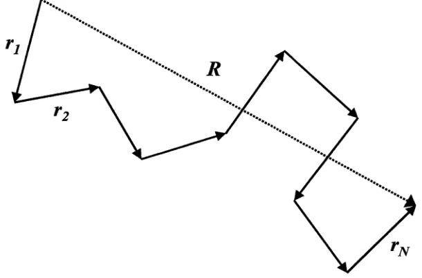
A simple model used for polymer chains is the freely jointed chain (FJC) model,1“'’9 Figure 2.1. The polymer chain is a series of N links of size a which orientate in­ dependently of each other. This is analogous to the trajectory of a random walk of fixed step size. The conformation of the chain can be described by either the set of the position vectors R n = (R0...R/v), or as the set of bond or step vectors r„ = (ri...rN) where

and the magnitude of rn is a, i.e., a = |rn| for all n. The size of the chain is determined by the end-to-end distance of the chain R, and is shown to be

Since the probability of the end-to-end distance of the chain being R is the same as it being —R, then the average < R > of R is zero. The size of the chain is determined from the average of the square of R. Let R be

R n R n —13 ^ 1 3 ^ 3 • • • 3 ^ • (2.1)

N

R — II v — Ro — V (2.2)

R = < R 2 > 1/2 (2.3)

and < R 2 > given by

2.1 . P o ly m e r C h a in M o d e ls 13

where ais the step size. For a FJC, where the orientation of the vectors is completely uncorrelated, < rn.rm > = 0 and n ^ m. Therefore eq 2.4 is

< R 2 > = N a2 (2.5)

Thus we say that the size of the freely jointed or ideal chain scales with N to the 1/2 power, or

R = V~Na. (2.6)

Although the FJC model is simple, the result < R 2 N a2 is quite general and holds for other models such as the freely rotating chain (FRC) model.2,4,9 The FRC model has a fixed angle between the bonds, therefore the orientation of the nearest neighbour vectors is correlated and < rn.rm > / 0 for n / m. However, as In — 7JiI increases, < rn.rm > approaches zero and < R 2 > ~ N is true for large N. For these models, the chain is not fully flexible and its flexibility is described by a term called the persistence length, /p,

Ip — a - Y h n > m ^ r n - r m > ^

o ) X ) n > m ^ ^

which is the length scale over which the chain is rigid. Substituting this into eq 2.4 gives

< R 2 > = A a 2 + 2 E „ a (l?/- a )

< R2 > = N a2 + 2Na(lp - a) (2.8) < R 2 > = Na 2{2(‘f ) - 1)

Therefore < R 2 > ~ Na 2 for large N, with the prefactor, (2(^i) — 1), varying from unity in the FJC model, to a large value for chains where correlation persists over a number of sequential bonds.

Random walk statistics can be used to describe the probability functions of the FJC. The probability of finding a chain whose end-to-end distance is between R and dR is p(R, N)dR. The probability distribution function, P ( R , N), of R of a sufficiently long chain ( N >> 1) is Gaussian:2-4,7,9

|2 -91 This general result comes from statistics and the central limit theorem.

The FJC model is very robust and mathematically simple to model. By having a equal to the persistence length, random walk statistics can be used. In Chapter

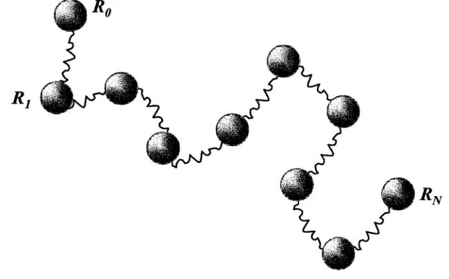
Figure 2.2: The beads-spring model.

The inherent difficulty lies in maintaining the N — 1 constraints of |R n — R m| = a, while tracking the positions of N beads. The solution is to change the links from a fixed length to a variable length which is selected from a Gaussian distribution. This model is referred to as the beads-springs model2,7 which recovers the random walk statistics and consequently still mimics an ideal chain. In simulation this model is the base upon which other potential interactions can be added, as for example interactions between the beads.

2 .1 .2 T h e G a u ssia n C h a in an d t h e B e a d -S p r in g M o d e l

A continuum model which is mathematically simple to model is the Gaussian chain model. This model makes the assumption that the bond vector or link r has a bond length chosne from the distribution

For a Gaussian chain, the position vector of the nth link can be written as R n (similar to the models previously described), then eq 2.10 gives the distribution of the bond vector, r n. The probability distribution of a chain with an end-to-end distance R n, P (R n), is given by

The Gaussian chain is most commonly described by the beads-springs model,2,7 Figure 2.2. The polymer chain is depicted as a series of N beads connected by

har-(2.10)

2.2 . T h e r m o d y n a m ic s and th e P o ly m e r S y ste m 15

monic springs, with an individual bead-spring component representing a statistical monomer unit of size a. If we let the spring constant be k, then the energy, U sprin g ,

of the chain is,

1 N

U spring = ~ k ~ R u - l ) 2) (2-12)

1 n- 1

At equilibrium the distribution function of the chain is proportional to exp(—U/ k BT) and k is

. 3 k BT k ---_a2 ~₁

where k B is Boltzmann’s constant and T is the temperature. Then the equilibrium distribution of the chain will be equivalent to eq 2.11. The Gaussian chain model depicted as beads-springs describes the properties of polymer chains on large length scales and is used quite frequently in polymer chain simulation.

2.2

T h er m o d y n a m ic s and th e P o ly m e r S y ste m

An important quantity for analysis of a thermodynamic system is the determina­ tion of the Helmholtz free energy, AF, and consists of both entropic and enthalpic contributions (AF = A E — T A S ) . ] The entropic term, T A S , describes the change in randomness that arises from the number of possible configurations of the chain, and the energy term, AE, describes the interactions of monomers within the chain or with other chains or surfaces. An ideal chain has no interactions amongst the monomers, hence there is no change in the interactions between the monomers and A E = 0. Therefore the ideal chain is purely entropic and is analogous to an ideal gas. The entropy, S is defined by Boltzmann’s principle as

S ~ k Bln(W) (2.14)

where W is the number of possible configurations of the polymer chain. The entropy change upon stretching and confining a chain is used in a theoretical treatment in this thesis. Therefore we will discuss this in the following sections.

2.2.1

Stretching a Polym er Chain

chain loses entropy or increases its free energy upon stretching according to1

AF = - T A S ~ —kBTlnP(R) (2.15)

We have already defined the probability distribution of R in eq 2.11, using this gives 3 knT R 2

2 N a 2 (2.16)

the change in free energy with extension R.

The change in energy is equal to the work required to stretch a chain. There­ fore, we can calculate the force for maintaining a given extension, R, by taking the derivative of eq 2.16 with respect to R ,

f = dF_ dR

3kBT

{^ x )R

The stretching behaviour of the chain is of a Hookean spring where the spring constant is inversely proportional to N. This is valid for small extensions, i.e., R « Na.

For large extensions of a polymer chain where the extension approaches the contour length of the chain, R =>> Na, the assumption of Gaussian statistics is not valid due to the small number of configurations available at such large extensions. A mathematical solution to this problem was to consider the distribution of R as electric dipoles being fully orientated by an applied field. This is applicable to extensions up to R = Na and was adapted by Kuhn and Grün as well as James and Guth3,4 and is simply the FJC of a finite number of inextensible links. Consider applying a force, f, in the x-direction to a single bond in the FJC. We let 6n be the angle of the bond with the x-axis and the bond configuration as x n = acos6n. Thus the bond configurational energy is —f x n, and the probability of its alignment value lying between x n and x n + dxn is proportional to

e xp ( f x n/ k BT)dxn (2.18)

The average extension distance of the bond, < x n > is given by

.. f - aXnexp(fxn/ k BT)dxn

< X" > = r - ^ M / k n T ) ^ ) = - (2.19)

The expression in the brackets may be rewritten as L ( f a / k BT), where £ is the Langevin function. Thus,

2.2 . T h e r m o d y n a m ic s and th e P o ly m e r S y ste m 17

projections of its N bonds on the x-axis and is

N

< x >— ^2 < xn > — LL ( f a / k ß T) (2.21)

n = l

where L is the contour length of the chain. The force necessary for extending a polymer chain a fixed distance < x > is

It is only necessary to use a more accurate mathematical description for polymer chain extensions larger than ~ (50N ]'/2)% of V < R 2 >. Note for this model, the parameter a is denoted as the Kuhn length which is a = < R 2 > /Na.

Although the FJC model using the Langevin function is more accurate than the Gaussian function for high extensions, it has been modified so as to more closely match observed high force behaviour in single polymer chain experiments.10,11 The extended FJC models involves the addition of the parameter, ksegment, which allows for the extensibility of the bonds as wTell as the alignment under an applied force. The expression for the extension of a polymer chain using the extended FJC model is,

Both the FJC and extended FJC model using the Langevin function are valid for fitting force curves for fully flexible polymer chains.

An alternative description of a polymer chain is the worm-like chain (WLC)

continuous curvature of the chain and describes its trajectory as a smooth curve that randomly changes direction. It is similar to the freely rotating chain in that the bond angles are fixed. The WLC model uses persistence length, lp instead of the Kuhn length for chain stiffness as well as the contour length as parameters for characterising the chain. In the absence of an applied force, the persistence length is equal to half the Kuhn length of the chain. Unlike the FJC model, there is no exact solution for the extension of the WLC by an applied force.12 However, a numerical solution has been obtained by treating the system quantum mechanically, that is as a field applied to an electric dipole and solving a differential equation equivalent to Schrödinger’s equation.9 The summarized equation was given by Bustamante et

kBT r _l ( < x >

1 T (2.22)

(2.23)

model. This model was developed by Porod and Kratky4 using the concept of

(2.24) This model is used to characterise stiff chains, although not exclusively.

C\

<P

o u a

C/5

cn

JU

C

o

c

<D

£ • l-M

T3

- - - - WLC

--- FJC (Langevin Spring)

---Gaussian Chain (Hookean Spring)

dimensionless extension, (x/a)

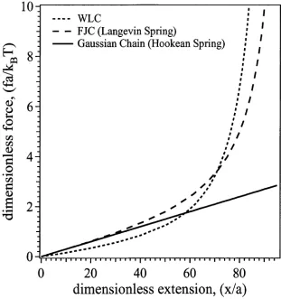
Figure 2.3: Dimensionless force, f a / ( K ß T ) : versus dimensionless extension, x / a, for the

different models: (1) a simple Gaussian chain; (2) the FJC; and (3) the WLC.

Hookean springs; (2) the FJC with Langevin springs and (3) the WLC. Note for small chain extensions the simple model of a Gaussian chain is adequate for extensions up to 1/2Na. For high extensions, the response of the polymer chain to an applied force is no longer linear and more sophisticated models are required such as the FJC and WLC models. For this reason the FJC and WLC models are used to fit force curves obtained in single molecule force microscopy experiments. We use the FJC, extended FJC and WLC models to fit our experimental force curves in Chapter 5.

2 .2 .2 P o ly m e r C o n fin e m e n t

The reduction in conformational entropy when an ideal chain goes from solution where its size is unrestricted (R ~ y/Na) to being confined within a slit of height H or a tube of diameter H is given by,

A S ~ kß x no. of times the chain ’Teels” a wall (2.25)

2.2 . T h e r m o d y n a m ic s and th e P o ly m e r S y ste m 19

▲

H

▼

Figure 2.4: An ideal chain trapped between two walls that are a distance H apart.

walk. However, a monomer near the wall is restricted and effectively loses the ability to move in one direction i.e., a three dimensional random walk is reduced to a two dimensional random walk. Therefore wre need to count the number of times that the chain comes into contact with the walls. As the chain is ideal, we know that the size of the portion of a chain which does not feel the walls is

H ~ am 1//2 (2.26)

where m is the number of monomers in the portion between the two walls. Therefore the number of contacts is,

N no. of monomers in chain

- = --- 7--- . , 2.27

77i no. ol monomers in bridge

and the change in entropy is

A S ~ —kn — (2.28)

m However, since m ~ H 2/ a2 then

N a 2

(2.29) A S ~ - k B- —

The compression of an ideal chain between two parallel plates of infinite size is analogous to a chain trapped in a pipe (see Figure 2.4). The free energy penalty of confinement is given by,1,14

Na2

F ~ (2.30)

2 .2 .3 P o ly m e r S o lv e n t T y p e s

All our previous sections have considered the polymer chain as ideal. However a polymer chain in solution rarely is ideal and its behaviour is greatly influenced by the solvent in which it is dissolved. There are three possible types of solvents or solutions for polymer chains which are nominally called good, poor or 0 (an ideal chain). A good solvent has interactions between itself and the solvent molecules being energetically favourable which results in the chain becoming swollen. A poor solvent means the monomers in the chain prefer to interact with themselves, rather than with solvent molecules. This has the effect of causing the chain to collapse as the monomers in the chain minimise their contact with the solvent molecules. A 0 solvent has a balance in the energy associated with repulsive (two-body) monomer- monomer interactions and the energy of monomer solvent interactions.

The interaction of a chain with itself is known as the excluded volume effect. Most notably it has been studied by Kuhn and Flory2’3,6 who determined the rela­ tionship of Rg wdth N as,

R « N ua (2.31)

where v is called the Flory exponent and varies according to temperature for a given polymer/solvent system.

The Flory argument for determining the size of a polymer chain in a good solvent involves balancing two effects, an excluded volume interaction which causes the coil to swell and an elastic energy that causes the chain to contract. We can therefore show this balance in the free energy of the chain:

F = U - T S (2.32)

where U involves the excluded volume and monomer-solvent interactions and T S the entropy of an ideal chain. The repulsive interaction potential for excluded volume can be expressed as a virial expansion,

U = V k BT ( B n2 + + Dr f + ...) (2.33)

where V is the volume of the chain and is proportional to the chain size cubed (V ~ R 3), 7] = N / V is the concentration of monomers, and B, C and D are virial coefficients. We can neglect the higher order terms as the density of monomers in the coil is small. Therefore, the repulsive interaction potential is,

U = V k ß T B i f (2.34)

2 .2 . T h e r m o d y n a m ic s and th e P o ly m e r S y s te m 21

from that of an ideal chain, then using the result for the ideal chain (see eq 2.16) and eq 2.34, the total free energy of the chain is,

F / k BT = V B r f + -3 Ä5

2 No? (2.35)

Introducing o, the swelling coefficient,

a =

N d 2

into eq 2.35 gives,

B V N 3 2

F/kfil ~ — - — — 4 ~ “ O '

(2.36)

(2.37) a3 a 3 2

The size of the polymer chain can be estimated by finding the minimum of F with respect to a. For dF/da = 0, the size of the chain is

R ~ ( l l ) 1/5aAf3/5

a3 (2.38)

The exponent 3/5 corresponds to the Flory exponent is v = 3/5 in eq 2.31.

A polymer chain in a poor solvent has the configuration of a spherical globule. This configuration minimises the surface area of the polymer chain and hence its interaction with the solvent. The volume of the spherical globule is V = 4/37TR? ~ a3N, where R is the radius of the sphere and the size of the chain. Therefore the size of a polymer chain in a poor solvent scales as,1,5

R « aTV1/3. (2.39)

For the ideal chain, the second virial coefficient is equal to zero {B = 0), resulting in the repulsive interaction potential, eq 2.34, being zero and the total free energy of the chain given by eq 2.16.

In summary the size of the polymer chains in the different solvents scales with N according to:1-3,5-9,15

R (J « iV3/5a a swollen chain

R (J ~ N ]/‘2a an ideal chain (2.40) R (J « N ]/*a a globule

2.3

S im u la tio n M e th o d s

Another method used in conjunction with theory to study single polymer chains is simulation. In our studies, we have used Langevin simulation exclusively. We will first discuss molecular dynamics as it is a more commonly used simulation, then the Langevin simulation comparing the two techniques and reasoning for our choice of simulation method.

2 .3 .1 M o le c u la r D y n a m ic s

Molecular Dynamics (MD) is able to calculate properties of a system, both static and dynamical by solving numerically Newton’s laws of motion.15-18 MD simulation involves a system of N particles placed within a cubic cell of constant volume, wTherc the initial coordinates of the particles, r ?(0), are arbitrarily chosen. The trajectories of the particles which interact via a potential are tracked. The coordinates of the particles are then determined after a short timcstep using Newton’s equations of motion. An example of the scheme of an MD simulation is the following. Using the finite difference method, a prediction is made for time t + At, for the particles’ coordinates, velocities and accelerations based on their current values. The forces and accelerations can then be calculated from the new coordinates using f, — where f2 is the force, m, is the mass and a, is the acceleration of a particle i. Using the new accelerations, the predicted coordinates, velocities etc. are corrected. Lastly, properties of the system such as energy, density are calculated before returning to the first step of making a prediction. This is one method of treating the equations of motion as first order differential equations.

2 .3 . S im u la tio n M e th o d s 23

the collective motion of molecules which occurs in diffusion and hydrodynamic flow as these occur over much longer timescales. To do this requires the use of coarse grain models. These have large length scales where the fluid system behaves as a continuum. The following simulation method uses this model.

2 .3 .2 L a n g e v in D y n a m ic s

The Langevin Dynamics is often called Brownian Dynamics and uses a dynamical equation of motion to describe the interaction of a large Brownian particle with fluid molecules.2,7,17 The time and length scales used in a Langevin simulation are sufficiently large that inertia of the particles is negligible. Therefore Newton’s law of motion, F = ma, is F = 0. The simulation calculates new coordinates of the Brownian particle with the sum of the forces acting on it are set to zero. This description is coarse grained and docs describe the system microscopically but not to the same molecular detail as in MD. This is because the dynamical properties we are interested in calculating for a polymer system are mesoscopic, z.e., the lengthscale wre are interested in is not Angstrom but of the micron scale. The solvent molecules are considered as a viscous continuum through which the particles move.

The behaviour of a Brownian particle in a solvent can be considered as a spherical particle that is buffeted by solvent molecules that collectively impart momentum to the particle. The particle motion was described by Einstein as a random walk with a root-mean-square displacement x at time t as10

x = (2 D t ) '/2 (2.41)

and D is the diffusion coefficient. The motion of the particle is also retarded by a frictional force F that is proportional to particle’s velocity, Vr,

F = ~CV (2.42)

where £ is the friction constant. This holds for the condition that the particle is smooth and the velocity is not too large. An equation relating kinetic energy to both the diffusion coefficient and friction constant is2,7,15

DC = k BT (2.43)

where kBT is the thermal energy and is known as the Einstein relation. For a spherical particle £ is determined from Stoke’s law,

£ = 6nr]a (2.44)

the Stokes-Einstein relation for a spherical particle diffusing through a medium

D = -L tL (2.45)

Gnrja

We then apply a continuous potential field U(x) to the Brownian particle which experiences a force, —dU/dx. The particle then moves with an average velocity7

V = JJJL

C dx (2.46)

through the solvent. If it is assumed that the effect of the Brownian motion is negligible, then from the last equation the particle displacement satisfies

dx 1 dU

dt £ dx

and the particle moves towards a decreasing potential, stopping when it reaches the minimum.

If there is Brownian motion, then the velocity of the particle fluctuates around the average value determined in eq 2.46. To account for these fluctuations, a proba­ bility function, g(t), that randomly varies with time, is added to the right hand side of eq 2.47

+

9(t)

dx 1 dU

dt £ dx

If the velocity fluctuations is the same for both the presence and absence of a field, then the mean and variance of g(t) is

< g(t) > = 0, < g{t)g{t') >= 2DS{t - t') (2.49)

where D is diffusion coefficient and has the following relation,7,19

D = k BT

c

known as the Einstein relation. The distribution of g(t) can then be assumed to be Gaussian. Equation 2.48 is known as the Langevin equation.

Equations 2.48 and 2.49 describe mathematically the motion of a Brownian par­ ticle in a potential field. If we integrate the Langevin equation from t to t -f At, and discretise with respect to time then

I o r 7

x(t -I- At) = x(t) — --Q—A t + G(t) (2.51)

2.4 . S u m m a r y 25

t to t + A t and has a mean and variance of

< G(t) >= 0, < G(t)G(t') >= 2DSw At. (2.52)

For determining how far a particle moves with time, t, we use the root mean square (r.m.s.) displacement < x 2 > 1//2 and not the mean displacement < x > which is equal to zero. The r.m.s. displacement is analogous to the standard deviation of the Gaussian distribution function G(t) and is15,19

< x2 > l/2= (2DAt)l/2. (2.53)

In Chapter 6, we use Langevin Dynamics in our simulations for investigating the dynamical behaviour of a single polymer chain.

2.3.3

R adius of G yration

In order to determine whether the chain has equilibrated or not, we calculate the radius of gyration, R g, of the chain which is,1-9,15

Rl

The radius of gyration is equivalent to the square of the average distance between the centre of mass of the polymer and its segments. The location of the centre of mass is

Rg = L E R - (2-55)

iV n - 1

and R (J can be written as

R]

n — 1

The chain is said to have equilibrated once the value of R y is constant with respect to time.

2.4

S u m m a ry

REFERENCES 27

R eferen ces

[1] de Gennes, P. -G. Scaling Concepts in Polymer Physics; Cornell University Press: Ithaca, 197 9.

[2] Doi, M.; Edwards, S. F. The Theory of Polymer Dynamics; Oxford University Press: Oxford, 1986.

[3] Flory, P. J. Principles of Polymer Chemistry; Cornell University Press: Ithaca, 1992.

[4] Flory, P. J. Statistical Mechanics of Chain Molecules; Hanser Publishers: New York, 1989.

[5] Evans, D. F.; Wennerström, H. The Colloidal Domain: Where Physics, Chem­ istry and Biology Meet, 2nd. ed.; Wiley-VCH: New York, 1999.

[6] Fleer, G. J.; Cohen Stuart, M. A.; Scheutjens, J. M. H. M.; Cosgrove, T.; Vincent, B. Polymers at Interfaces; Chapman & Hall: London, 1993.

[7] Doi, M. Introduction to Polymer Physics’, Clarendon Press: Oxford, 1997. [8] Israelachvili, J. Intermolecular and Surface Forces, 2nd. ed.; Academic Press:

London,1992.

[9] Yamakawa, H. Modern Theory of Polymer Solutions; Harper & Row: New York, 1971.

[10] Smith, S. B.; Cui, Y.; Bustamante, C. Science 1996, 271, 795.

[11] Rief, M.; Oesterhelt, F.; Heymann, B.; Gaub, H. E. Science 1997, 275, 1295. [12] Fixman, M.; Kovac, J. Journal of Chemical Physics 1973, 58, 1564.

[13] Bustamante, C.; Marko, J. F.; Siggia, E. D.; Smith, S. Science 1994, 265, 1599. [14] Guffond, M. C.; Williams, D. R. M.; Sevick, E. M. Langmuir 1997, 13, 5691. [15] Hamley, I. W. Introduction to Soft Matter, John Wiley & Sons: New York,

[16] Heermann, D. W. Computer Simulation Methods in Theoretical Physics; Springer-Verlag: Berlin, 1986.

[17] Hansen, J. R; McDonald, I. R. Theory of Simple Liquids, 2nd ed.; Academic Press: London, 1986.

[18] Allen, M. P.; Tildesley, D. J. Computer Simulation of Liquids; Clarendon Press: Oxford, 1990.

C hapter 3

A tom ic Force M icroscope: T he

Instrum ent and Its U se

3.1

I n tro d u c tio n to th e A to m ic Force M icroscope

The atom ic force microscope (AFM ), or as it is otherwise known the scanning

force microscope, was invented by Binnig et al. in 1986.1 The AFM is able to image

surfaces and is an im portant technique used in a num ber of different fields including

sem iconductor processing, m aterial science, polymers, biology and biom aterials, to

name only a few. The AFM can also be used to probe the adhesive and elastic

properties of sample surfaces and for nanom anipulation. As the AFM has a force

sensitivity of only a few picoNewtons, it is capable of probing fundam ental forces

including attractiv e van der Waals forces, electrostatic forces, capillary forces and

magnetic forces. The advent of the fluid cell has enabled the AFM to measure forces

in a fluid environm ent enabling the study of electrostatic forces between dissolved

ions and other charged species on the probe tip and sample surface,4 biological m a­

terials,3,5-11 colloidal forces12-14 and the nanom anipulation of polym er chains.13,15-26

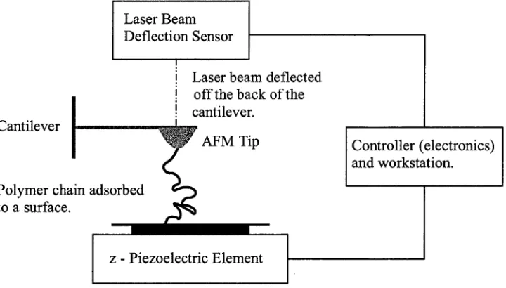
Figure 3.1 shows the essential com ponents in an AFM. The AFM uses a probe

consisting of a sharp tip attach ed to a flexible cantilever to determ ine the properties

of a sample surface. Forces acting between the probe tip and sample cause the

cantilever to deflect which is measured by bouncing a laser beam off the back of the

cantilever. This detection m ethod uses a laser beam deflection sensor and is known

as the optical or light lever m ethod. The AFM can create three dimensional images

of a sample surface from these deflections w ith a spatial resolution of nanom eters

and a vertical resolution of A ngstrom s by raster scanning the sam ple plane in the

x-y direction using a com puter controlled piezoelectric stage. In addition, the AFM

measures force curves by moving the probe tip perpendicular to the sample plane,

i.e., in the z-direction. The range of forces an AFM can detect and measure forces

Laser Beam Deflection Sensor

Laser beam deflected off the back of the cantilever.

Polymer chain ads< to a surface. Cantilever

Controller (electronics) and workstation.

z - Piezoelectric Element

Figure 3.1: Schematic diagram of an atomic force microscope (AFM). The AFM tip is

attached to a cantilever type spring. The sensor monitors any resulting deflections in the

cantilever due to forces acting upon the tip. The force between the tip and the sample

surface can be precisely controlled by the controller electronics and workstation using the

output from the deflection sensor and the piezoelectric element to determine the height

(z-displacement) of the AFM tip from the sample surface.

3.2 . C a n tilev e r and P r o b e T ip s 31

Figure 3.2: A schematic of the extension of an end-tethered chain using an AFM probe. D is the z-displacement of the piezo scanner, x is the deflection of the cantilever, kc is the cantilever spring constant and kp the polymer spring constant and l is the length of the polymer chain extended. When there is no interaction between the probe tip and the sample surface, the tip-sample separation is equivalent to D.

deflect a small distance x, so as to be able the measure the force. Since x / D << 1/D, then tip-sample separation can be approximated as the z-displacement of the piezo, i.e., I ~ D.

In this chapter we discuss in Sections 3.2-3.4 the essential components of the AFM including manufacturer specifications, limitations and calibration techniques. In Section 3.5 we briefly describe the various operational modes used for imaging and measuring forces using the AFM. Section 3.6 describes in detail the conversion of the raw data into force versus distance curves. The various sample surface clean­ ing techniques are described in Section 3.7 and lastly in Section 3.8 we describe experimental modifications made to the AFM in order to conduct our experiments.

3.2

C a n tilev er and P r o b e T ip s

manufacturer quotes a range of 0.4 to 0.7 gm) leads in a variation of the spring constants. As the spring constant is proportional to the thickness cubed, the spring constant would have a range from 0.017 to 0.095 Nrn-1. The specifications of the probe as stated by the manufacturer are as follows: the cantilever is v-shaped with a length of 200 pm, the leg width of the cantilever is 30 pm, the tip radius has a range of 20-60 nm and the resonant frequency is 5-50 kHz. Although a convenient way of measuring the force, there are inherent problems in this technique. Specifically, when the tip is under a load (in contact with the sample surface) it is no longer linear but describes an arc. This reduces the accuracy of the measured adhesion forces due to surface shearing. Also the vibrational modes of the cantilever are not simple, making theoretical treatments difficult.

3 .2 .1 S p r in g C o n s ta n t C a lib r a tio n

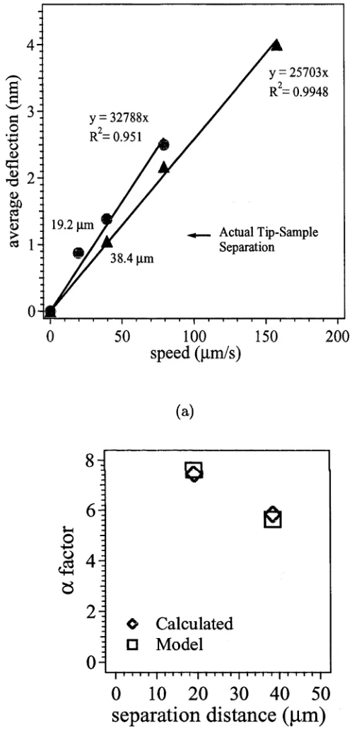
In determining the spring constant of the cantilever, it is important to note that the AFM can only measure a change in the deflection. The gravimetric method30 measures the static deflection of a cantilever by by end-loading it with a known mass. This calibration technique has a reported error of ~ 10%. An alternative method that also end-loads the cantilever measures the change in resonant frequency of the cantilever31 and has an error range of 5 — 10%. The calibration of spring constants by resonant methods is a popular technique that is continually being refined both experimentally32 and theoretically.33

3.2. C a n tilev er and P r o b e T ip s 33

; 19.2 fim

Actual Tip-Sample Separation 38.4 pm

100

speed (pm/s)

(a)

o

- C Ö

Ö

8

6

4

2

0

0 10 20 30 40 50

separation distance (jam)

a

O Calculated

□ Model

(b)

Figure 3.3: An example of the plots used to determine the spring constant of the cantilever

for an AFM experiment. Figure (a) is the average deflection of the cantilever (nm) versus

speed (pm/s) for different tip-sample separations. Figure (b) is a plot of a-factor versus

the tip-sample separation (pm). In this instance, the solution was 0.3 wt% PEO in 0.45