Using Statistical Shape Decomposition and Conditional Models
.
White Rose Research Online URL for this paper:
http://eprints.whiterose.ac.uk/90967/
Version: Accepted Version
Article:
Pereanez, M., Lekadir, K., Castro-Mateos, I. et al. (3 more authors) (2015) Accurate
Segmentation of Vertebral Bodies and Processes Using Statistical Shape Decomposition
and Conditional Models. IEEE Transactions on Medical Imaging , 34 (8). 1627 -1639. ISSN
0278-0062
https://doi.org/10.1109/TMI.2015.2396774
[email protected] https://eprints.whiterose.ac.uk/ Reuse
Unless indicated otherwise, fulltext items are protected by copyright with all rights reserved. The copyright exception in section 29 of the Copyright, Designs and Patents Act 1988 allows the making of a single copy solely for the purpose of non-commercial research or private study within the limits of fair dealing. The publisher or other rights-holder may allow further reproduction and re-use of this version - refer to the White Rose Research Online record for this item. Where records identify the publisher as the copyright holder, users can verify any specific terms of use on the publisher’s website.
Takedown
If you consider content in White Rose Research Online to be in breach of UK law, please notify us by
Processes using Statistical Shape Decomposition
and Conditional Models
Marco Perea˜nez, Karim Lekadir, Isaac Castro-Mateos, Jos´e Maria Pozo, ´
Aron Laz´ary,
and Alejandro F. Frangi,
Fellow, IEEE
Abstract—Detailed segmentation of the vertebrae is an impor-tant pre-requisite in various applications of image-based spine assessment, surgery and biomechanical modeling. In particular, accurate segmentation of the processes is required for image-guided interventions, for example for optimal placement of bone grafts between the transverse processes. Furthermore, the geometry of the processes is now required in musculoskeletal models due to their interaction with the muscles and ligaments. In this paper, we present a new method for detailed segmentation of both the vertebral bodies and processes based on statistical shape decomposition and conditional models. The proposed technique is specifically developed with the aim to handle the complex geometry of the processes and the large variability between individuals. The key technical novelty in this work is the introduction of a part-based statistical decomposition of the vertebrae, such that the complexity of the subparts is effectively reduced, and model specificity is increased. Subsequently, in order to maintain the statistical and anatomic coherence of the ensemble, conditional models are used to model the sta-tistical inter-relationships between the different subparts. For shape reconstruction and segmentation, a robust model fitting procedure is used to exclude improbable inter-part relationships in the estimation of the shape parameters. Segmentation results based on a dataset of 30 healthy CT scans and a dataset of 10 pathological scans show a point-to-surface error improvement of 20% and 17% respectively, and the potential of the proposed technique for detailed vertebral modeling.
Index Terms—Vertebral segmentation, point distribution mod-els, part-based shape decomposition, conditional models.
I. INTRODUCTION
S
EGMENTATION of the vertebrae is an important pre-requisite for a number of clinical applications, ranging from the assessment of spinal disorders and image-guided surgery [1], [2] to biomechanical modeling for patient-specific planning of interventions [3], [4]. For such applications, in addition to the segmentation of the vertebral bodies, accurate and detailed knowledge of the vertebral processes is necessary (Fig. 1). For spinal fusion surgery, for example, precise delin-eation of the processes can lead to an improved placementMarco Perea˜nez is with the Center for Computational Imaging and Simulation Technologies in Biomedicine, Universitat Pompeu Fabra, 08018 Barcelona, Spain e-mail: ([email protected]).
Karim Lekadir is with the Center for Computational Imaging and Sim-ulation Technologies in Biomedicine, Universitat Pompeu Fabra, 08018 Barcelona, Spain.
Isaac Castro-Mateos, Jos´e Maria Pozo and Alejandro F. Frangi are with the Center for Computational Imaging and Simulation Technologies in Biomedicine, University of Sheffield, S1 3JD Sheffield, U.K.
´
Aron Laz´ary is with the National Center for Spinal Disorders, Kiralyhago u. 1-3., Budapest, Hungary, H-1126.
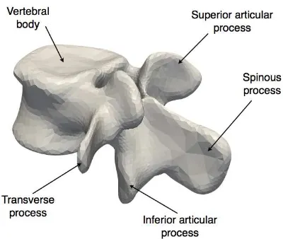
[image:2.612.338.538.271.440.2]of the bone graft between the transverse processes of the affected vertebrae [5]. In biomechanical modeling of the spine, accurate definition of the spinous process is also critical due its interaction with the ligaments and the muscles [6].
Figure 1. A lumbar vertebra and its main regions.
In practice, however, automatic and detailed segmentation of vertebrae, and in particular of its processes and pathological cases, has proven to be a difficult task due to the complexity of the shapes and the high variability between individuals. As shown in Figs. 1 and 2, the vertebral processes consist of various areas of distinct geometrical but equally complex char-acteristics, with several convex/concave structures, as well as thin lobe-like elongated regions. As shown in Fig. 2 (bottom), trauma patients with fractured vertebrae present statistically anomalous shapes that present a challenge for straightforward shape modeling. As a result, the precise modeling and seg-mentation of the vertebral processes remains a challenging research topic within spine imaging.
models for each vertebra. In contrast, Rasoulian et al. [18] combined all the vertebrae into a single shape model, together with a statistical pose model. In both cases, these methods consider at best a whole vertebra as the smallest unit for the construction of the SSM. Due to the large variability of the vertebrae in particular for pathological instances and at the processes, and the generally small number of samples available for training, the obtained models are typically too constraining and not flexible enough to localize the fine details and areas of high curvatures and complexity within the vertebral body and processes, as illustrated in Fig. 2.
In this paper, we present a new method for detailed mod-eling and segmentation of the vertebrae based on statistical shape decomposition. Multi-part shape models have been proposed in the literature with the aim to relax the shape constraints in the presence of a small number of training samples, or extract additional information in the relationship between objects to aid the segmentation process [22], [23], [24], [25]. Other methods have proposed subdivision of the parametric shape-space rather than the shapes themselves in order to better approximate the actual shape distribution of the object class [26], [27]. Nevertheless, such methods have not been applied to the vertebrae as the subdivision of such a complex shape is a non-trivial problem.
In this paper, we propose an algorithm for statistical de-composition of the vertebra, and for modeling the relationship between the parts. The proposed shape decomposition effec-tively reduces the complexity of each constituent model, while at the same time increasing their specificity. The proposed approach is particularly useful to model difficult regions of the vertebra such as the processes and pathological cases such as fractured vertebrae, thus improving segmentation accuracy. Subsequently, in order to maintain the coherence of the en-semble, conditional models are used to model the statistical inter-relationships between the different subparts. For spine image segmentation, a robust model fitting procedure is then introduced to exclude inconsistent inter-part relationships dur-ing the estimation of the shape parameters.
The segmentation accuracy of the proposed technique was tested on two Computed Tomography (CT) scan datasets. One dataset of 30 healthy, and a dataset of 10 pathological cases. Training was performed on the healthy population following a leave-one-out scheme (29 training, 1 testing) to test the healthy cases. And the complete healthy dataset to test the pathological cases.
This work is based on a conference paper [28], which we extend by developing a new statistical decomposition of the vertebrae, with more detailed evaluation of the properties of the algorithm and testing segmentation results on both healthy and pathological patients.
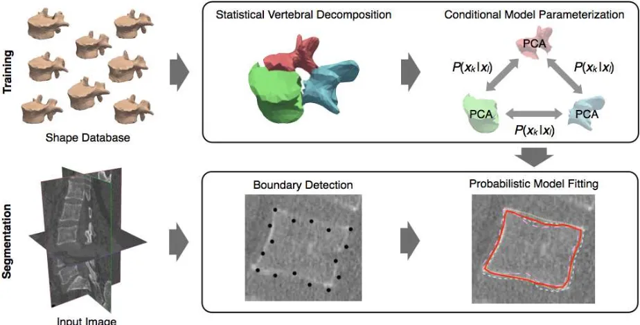
II. METHOD
The proposed framework consists of three main stages. First, in Section II-A, a subdivision of each vertebra into a number of subparts is proposed based on a statistically driven region decomposition. Subsequently, the conditional models describing the statistical inter-relationships between
the subparts are presented in Section II-B. Finally, a model fitting approach based on all pairwise conditional models is introduced in Section II-C2, with the aim to estimate the shape parameters for each subpart robustly during image segmentation. Figure 3 shows a schematic of the method’s workflow.
A. Statistical Vertebral Decomposition
A common problem in the representation of complex and highly variable anatomical objects using statistical shape mod-els is that usually there are too few available examples from which to obtain a sufficiently detailed representation of the population and its natural variability. In the case of the verte-bra, few samples are sufficient to obtain a gross approximation of the global shape distribution of a given population, but this is often not enough to encode the finer details of the vertebral processes (Fig. 2) or to represent instances that deviate far from the mean of the population. In this paper, we address these issues by developing a statistical part-based decomposi-tion to better encode the statistical variability of each region of the vertebra, and to better generalize to instances not present in the training set. However, such subdivision is not trivial as the statistical variability and geometrical complexity in the vertebra is uneven.
In this work, the proposed shape subdivision takes into account the statistical properties of the parts, and therefore provides a statistically coherent subdivision that minimizes bias towards any of its parts. More specifically, the proposed method ensures that the variability of the whole shape is equitably distributed into a specified number of regions such that Point Distribution Models (PDMs) constructed from these regions encode similar amounts of variability.
The algorithm has three parts: 1) seed placement, 2) initial region labeling, 3) statistical region optimization.
1) Seed Placement: In order to subdivide the shape into the desired number of regions, the user must specify the number of regionsK. Let us denotexi= (x1. . .xr)T,i= 1. . . Nthe
landmark-based shape representation of each vertebra, where
ris the number of landmarks,N is the number of shapes, and
¯
xis the mean shape computed from all shapesxi. The aim is
to subdivide¯xintoKsub-parts¯xk. We use the mean shapex¯
so that the result is not biased toward any one sample. After
K is specified an initial seed point is randomly selected from the vector ¯x. Then, the remaining K−1 points are selected such that the Euclidean distance between thekthpoint and all previously selected seed points is maximized. This strategy ensures that the initial region seeds are uniformly distributed throughout the shape, and helps to minimize computational time during the statistical region optimization (step 3) of the algorithm. See Algorithm 1.
2) Initial Region Labeling: Based on theK seed points, a partition intoK regionsRk is obtained. Initially, each region Rk contains only its corresponding seed point, and all points
that have not been assigned to any region are said to belong to the null region R0. We then iterate through the newly
Figure 2. Examples of suboptimal segmentations in areas of complex geometry and high curvature (top), and fractured vertebrae (bottom). These segmentations (in blue) were obtained using the image search method [21] described in section II-C1 and constrained with a whole-vertebra PDM.
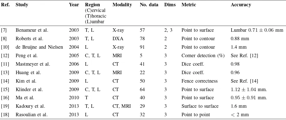
Table I
STATE-OF-THE-ART TABLE.
Ref. Study Year Region
(C)ervical (T)horacic (L)umbar
Modality No. data Dims Metric Accuracy
[7] Benameur et al. 2003 T, L X-ray 57 2, 3 Point to surface Lumbar0.71±0.06mm
[8] Roberts et al. 2003 T, L DXA 78 2 Point to contour 0.88 mm
[10] de Bruijne and Nielsen 2004 L X-ray 91 2 Point to contour 1.4 mm
[12] Peng et al. 2005 C, T, L MRI 5 3 Corner detection (%) See Ref. [12]
[11] Mastmeyer et al. 2006 L CT 41 3 Dice coeff. 0.98
[13] Huang et al. 2009 C, T, L MRI 22 3 Dice coeff. 0.96
[14] Kim et al. 2009 L CT 50 3 Fence correctness See Ref. [14]
[15] Klinder et al. 2009 C, T, L CT 64 3 Point to surface 1.12±1.04mm.
[16] Ma et al. 2010 T CT 40 3 Point to surface 0.95±0.91mm.
[19] Kadoury et al. 2013 T, L CT, MRI 29 3 Surface to surface 1.6 mm
[18] Rasoulian et al. 2013 L CT 32 3 Point to point <2 mm
points belong to thenullregionR0, they are removed fromR0
and assigned to the current region Rk. We repeat this process
until thenullregion is empty, and all points in the mesh have been added to some region Rk.
Based on the obtained regions Rk we can now subdivide
shapes xi into subparts xi,k. From the nature of the
initial-ization and initial region label assignment these regions have approximately the same number of points, however, they may vary greatly in terms of their variance across the population, particularly regions at the processes will contain a higher variance than regions on the vertebral body. For this reason, an optimization is required in order to equalize the amount of
variability of all regions so that modeling of the vertebra is not biased by any region.
Figure 3. The proposed method consists of two training steps (top): 1) vertebral shape subdivision (See Sec. II-A), and 2) construction of conditional models (See Sec. II-B). The segmentation process also has two steps (bottom): 1) initial boundary detection (See Sec. II-C1), and 2) Multiple model fittings given all conditioning subshapes (See Sec. II-C2). These model fittings are shown in dotted lines (bottom right). The final segmentation is computed as the median estimation of all model fittings (continuous red line).
covariance matrix
C= 1
N−1
N X
i=1
(xi−¯x)(xi−¯x)T, (1)
and the total population variance as
Vartotal =tr(C). (2)
Similarly we define the regional covariance matrices as
Ck=
1
N−1
N X
i=1
(xi,k−¯xk)(xi,k−¯xk)T, (3)
and the regional variances as
Vark =tr(Ck). (4)
The algorithm first determines the target variance for each region as
Vartarget=
Vartotal
K . (5)
Then, the algorithm iterates through the regions and computes the variance of the current region. If the variance of the current region Vark is less than the target variance Vartarget, we
reassign all adjacent points to the perimeter of the current region Rk from adjacent regions Rl, k 6= l. In Algorithm
2, line 14, we denote this operation expandPerimeter. Similarly, If the variance of the current region Vark is greater
than the target variance Vartarget we reassign all points at the
perimeter of the current region to those regions adjacent to it. In Algorithm 2, line 20, we denote this point reassignment with the function nameshrinkPerimeter.
The algorithm iterates until the standard deviation of all region variances falls below 5% of the target variance, i.e.,
std(Vark)<0.05·Vartarget (see Algorithm 2), or no further
changes in region variances occur. Once the optimization converges the vertebral shape is effectively subdivided into regions of similar variability. It is worth noting that for all experimental results reported in the results section (Sec. III) of this paper, the shapexi being tested was removed from the
training set, i.e, leave-one-out scheme.
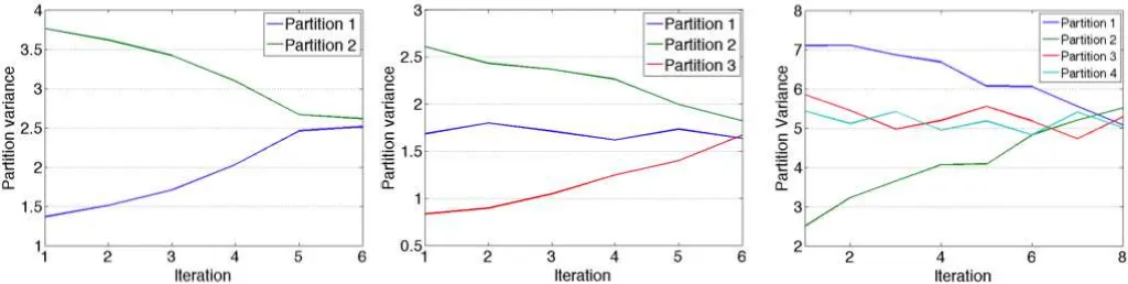
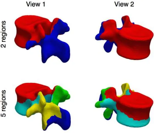
Figure 5 shows examples of the convergence of the al-gorithm for three different shape subdivisions (2, 3 and 4 regions). The figure shows how region variances at iteration 1 are unevenly distributed across the shape and how they converge for an even distribution of the variance. Figure 4 shows two examples of the final vertebral decomposition for 2 and 5 regions. Note that the region/s describing the vertebral processes are comprised of fewer points indicating higher variability, whereas the regions at the vertebral body are larger. Also in the 5-region case more regions are necessary to represent the variability at the processes, whereas only 2 larger regions represent the vertebral body.
B. Conditional Model Parametrization
In the previous section we subdivided the shape of all vertebrae into K subparts xi,k, k = 1, . . . , K. The aim
of this section is to describe the statistical modeling of the inter-part probability distributions, i.e. P(xi,k|xi,l), where k, l = 1, . . . , K andk6=l. More specifically, we would like to compute a PDM for each partxi,k based on its conditional
relationship with xi,l, that is, a mean ¯xk|l and covariance
matrix Σk|l. In this paper, we choose to model P(xi,k|xi,l)
using a normal probability distribution. Thus, the conditional mean and covariance estimates that relate shapesxi,k, andxi,l
[image:5.612.47.295.365.537.2]Figure 5. Illustration of the region variance evolution produced by the statistical vertebral decomposition algorithm. It can be seen that the variability of the subparts converges to a nearly equal value.
Algorithm 1 Seed placement 1: Input:Number of regions:K 2: Input:Mean shape:¯x
3: ⊲Randomly determine initial region seed. 4: [point,pointIndex]=getRandomPoint(¯x)
5: seeds(1) =point
6: ¯x(pointIndex) =[] ⊲Delete seed point from¯x.
7: fork= 2→K ⊲For all regions. 8: maxDist= 0
9: nP oints=getNumberOfPoints(¯x) 10: nSeeds=getNumberOfPoints(seeds)
11: forp= 1→nP oints ⊲For all points in the shape.
12: fors= 1→nSeeds ⊲For all seed points. 13: Comment: Get distance from pointpto all seeds. 14: dists(s)= getDist(x¯(p),seeds(s))
15: end for
16: distsSum=sum(dists) ⊲Sum dists to all seeds.
17: ⊲If current point is further from all seeds than previous point, store index.
18: ifdistsSum > maxDist 19: maxDist=distsSum 20: nextSeed=p 21: end if
22: end for
23:
24: seeds(k) =¯x(nextSeed) ⊲Store next seed. 25: x¯(nextSeed) =[] ⊲Delete seed point fromx. 26: end for
27: Output:seeds
¯
xk|l=¯xk+ΣklΣll−1(xi,l−¯xl) (6)
Σk|l=Σkk−ΣklΣ−ll1Σlk, (7)
where the covariance matrices in Eqs. 6 and 7 are obtained from a block covariance matrix
Algorithm 2 Statistical region optimization
1: Input:Region point matrices:X(1). . .X(K) 2: Input:Region point connectivity:V(1). . .X(K) 3: Input:Number of regions:K
4: fork= 1→K ⊲For all regions. 5: Ck=cov(X(k)) ⊲Covariance of region k. 6: regV ar(i) =trace(Ck) ⊲Get region variance. 7: end for
8: varT otal=sum(regV ar) ⊲Sum all region variances. 9: varT arget=varT otal/K ⊲Get target variance. 10: allowedDispersion= 0.05∗varT arget ⊲5% of target
variance
11: dispersion=std(regV ar)⊲Get region variances’ dispersion.
12: whiledispersion > allowedDispersion
13: fori= 1→K ⊲For all regions.
14: ifregV ar(i)< varT arget ⊲If Var is below target. 15: X(i) =expandPerimeter(X(i),V(i)) ⊲Enlarge region.
16: forj= 1→K ⊲Update region variances. 17: Ck=cov(X(j))
18: regV ar(j) =trace(Ck) 19: end for
20: else ⊲If region variance is above target. 21: X(i) =shrinkPerimeter(X(i),V(i)) ⊲Contract region.
22: forj= 1→K ⊲Update region variances. 23: Ck=cov(X(j))
24: regV ar(j) =trace(Ck) 25: end for
26: end if
27: end for
28: dispersion=std(regV ar) ⊲Update variance dispersion. 29: end while
Figure 4. Examples of the obtained statistical decomposition with 2 regions (top), and 5 regions (bottom). The left and right columns show a latero-posterior and latero-anterior views. In the 5-region case more regions are necessary to represent the processes due to their high variability.
Σ=
Σkk Σkl
ΣTkl Σll
. (8)
Through eigendecomposition of Eq. 7 we obtain Eq. 9, which provides the eigenvalues Λk|l, and eigenvectors Φk|l that
represent the conditional variability between shapes xi,k and
xi,l.
Σk|l=Φk|lΛk|lΦTk|l, (9)
Putting Eqs. 6 and 9 together we obtain the new conditional models
Ωk|l= (¯xk|l,Φk|l,Λk|l) (10)
that we will use to constrain the image segmentation process. In order to compute the conditional mean ¯xk|l and
co-variance matrix Σk|l we need to compute the inverse of the
covariance matrix of the predictor shapeΣ−ll1. However, as the dimensionality of the shapes is much larger than the number of training samples available, the sample covariance matrix becomes singular, and cannot be inverted. A solution to this is using ridge regression [30], where a small constant is added to the diagonal of the covariance matrixΣˆll=Σll+ǫI, where
Iis the identity matrix.
The computational burden of inverting matrices representing several thousands of points can be considerable, especially given that we need to compute a conditional PDM for each pair-wise relationship between the shape subdivisions, and so the number of matrix inversions needed to compute Eqs. 6 and 7 grows linearly with K. We address this issue by reducing the dimensionality of the problem using Principal Component Analysis (PCA) on the subshapes xi,k prior to computation
of the mean and covariance matrix as follows [31]. Given subshapesxi,k represented as,
xi,k=xk+Φkbi,k, (11)
then their parametric representation is
bi,k =ΦTk(xi,k−x¯k). (12)
Now let us denote Bk the column-wise concatenation of
parametric shape vectorsbi,kfrom equation 12. With this new
representation of the shapes, the cross-covariance matrixΣkl
on Eqs. 6, 7 and 8 becomes
Σ(klb)= 1
N−1BkB
T
l, (13)
where the superscript (b) in Eq. 13 indicates that the covari-ance matrix is computed from parametric shape vectorsbi,k.
The block covariance matrix of Eq. 8 can now be replaced by
Σ(b)=
"
Λk Σ
(b)
kl
Σ(klb)T Λl #
, (14)
whereΛk andΛl are diagonal eigenvalue matrices obtained
through eigendecomposition of the original subshapesxi,kand
xi,l.
With this new representation Eqs. 6 and 7 can be rewritten as
¯
xk|l=¯xk+Φk(Σ
(b)
klΛ
−1
l bi,l) (15)
Σk|l=Φk(Λk−Σ
(b)
kl Λ
−1
l Σ
(b)
kl T
)ΦTk, (16) where the expression in parenthesis on Eq. 15 is the regressed parametric shape estimateb¯k|l, i.e.,
¯ bk|l=Σ
(b)
klΛ
−1
l bi,l, (17)
and the expression in parenthesis on Eq. 16 is the conditional model variance
Λk|l=Λk−Σ( b)
kl Λ
−1
l Σ
(b)
kl T
(18)
required to obtain the desired modelΩk|l= (¯xk|l,Φk,Λk|l).
The proposed shape subdivision and conditional model parameterization have two important goals. First, it decreases the over-constraining nature of the global model caused by the dimensionality disparity between the available samples and dimensionality of the shapes. And second, and as detailed in next section, the inter-part conditioning is used as a mechanism to find the optimal domain of valid subregions and exclude incorrect localized segmentations due to insufficient image information.
C. Image Segmentation
1) Boundary Detection: To detect the vertebral boundary in the image we followed the feature training method introduced in [21]. Training was performed on the database of 30 healthy patients detailed in section III-A leaving the test instance out at each trial. The features tested were:
1) Directional derivative along the normal profile pointing outwards.
2) Directional derivative along the normal profile pointing inwards.
3) Maximum intensity profile value. 4) Minimum intensity profile value.
framework. A greedy optimization heuristic was used where at each iteration a set of uniformly distributed weightsw= [0,1]
was used for segmentation and the best performing weight was selected based on segmentation accuracy. At the next iteration a new set of weights was uniformly chosen within a neighborhood of the best weight from the previous iteration. This procedure was repeated until no significant improvements in segmentation accuracy were obtained. For more details on the optimization procedure please refer to [21].
After individual optimization of the features, the best-performing three features were chosen and normalized. The selected features were: 1) the directional derivative along the outward-pointing normal, 2) the image intensity, and 3) the distance between the current point candidate and its previous location. The corresponding feature weights were:w1= 0.55,
w2= 0.25, andw3= 0.20.
E=w1(nˆ(pr)· ∇I(p′r)) +w2I(p′r) +w3kp′r−prk2.(19)
Eq. 19 shows the energy function maximized during image search, where I is the intensity image, pr is the current
position of the landmark r, p′r is a vector of candidate landmark positions normally and outwardly oriented with respect to the surface mesh atpr, andˆnis the normal direction
atpr.
The segmentation process was initialized by rigidly aligning the mean vertebral shape, for the given structure (L1-L5), with a manually selected point placed roughly at the center of mass of the vertebral body on a sagittal view of the image. Then the algorithm determined the optimal placement of each landmark in the mesh based on minimization of Eq. 19.
Let us denote the resulting feature pointsx′. At this pointx′
can be subdivided into K statistically optimized regionsx′k, k= 1. . . K, as described in Sec. II-A. The following section describes the process through which information from all other
K−1subregions inform the optimal shape parametersbk of
x′k with the goal of maintaining anatomical coherence of the
ensemble of parts.
2) Probabilistic Model Fitting: To preserve the anatomic validity of the segmentation in spite of the shape decompo-sition, the estimation of the shape parameters must be car-ried out by considering all pairwise conditional probabilities
P(xi,k|xi,l). We first calculate the initial shape parameters
bi,kby projecting the boundary feature points (obtained during
image search) onto the standard PDM of xi,k. Subsequently,
we calculate K−1 shape parameters bi,k|l by considering
the K−1shape constraints formed by the conditional mean parameter ¯bk|l and its corresponding bounds λk|l obtained
from the diagonal of matrix Λk|l, i.e.,
bi,k|l=
b0i,k if |b0i,k−¯bk|l| ≤3 p
λk|l
¯ bk|l+ 3
p
λk|l if b0i,k >b¯k|l+ 3 p
λk|l
¯ bk|l−3
p
λk|l if b0i,k <b¯k|l−3 p
λk|l
(20)
Equation 20 is applied to each shape pair {xi,k,xi,l} as
follows:
Let us denote this subregion the conditional prediction interval Tk|l (See Alg. 3, line 15).
2) If b0i,k is inside the conditional prediction interval,
b0i,k ∈ Tk|l, we consider the conditional prediction
bi,k|las the same asb0i,k. Thus, no extra information is
provided by the conditional model.
3) In case b0i,k is outside Tk|l, then it is projected to
obtain the closest point inside Ti,k|l. This point is then
considered the prediction bi,k|l.
The difficulty with this approach is that at the segmentation stage, all subparts are being segmented and therefore there is uncertainty surrounding the correctness of the different conditioning shapes xi,l in P(xi,k|xi,l). This can lead to
inaccurate constraining and parameter estimation of xi,k|l if
some of thexi,l,l= 1. . . K,k6=l are erroneous during the
segmentation procedure. To exclude these values and obtain a consensual and robust estimation of the shape parameters, we use the marginal median (component-wise median) as the final estimation ofbi,k|l, i.e.,
bf inali,k|l =median(bi,k|l). (21)
Algorithm 3 presents the step by step model fitting procedure described in this section.
III. RESULTS A. Data
We first trained and validated our method using a database of lumbar spine (L1-L5) CT images of 30 healthy patients reporting lower back pain. The images were collected at the National Center for Spinal Disorders (Budapest, Hungary). The data were acquired with a Hitachi Presto CT scanner. No contrast agent was administered to the patients. The volumes have an in-plane resolution of 0.608 ×0.608 mm and slice spacing of 0.62 mm. Patients were 13 males and 17 females with a mean age of 40 (age interval: 27-62 years). Those patients were selected for participating in the European Commission funded MySpine project.
Furthermore, to assess the strength of the proposed tech-nique in the presence of abnormalities, a second set of 10 scans were obtained to evaluate segmentation. The images were obtained from a publicly available database [32] of CT scans of adult patients with varying types of pathologies including pathological curvature (scoliotic and kyphotic), and fractured vertebrae. The data were acquired at the Department of Radiology, University of Washington, Seattle, USA. The images were acquired with General Electric multidetector CT scanners and a standard bone algorithm. For our purposes, 10 image volumes containing full lumbar spines (L1-L5) were randomly selected and manually segmented. The images have varying in-plane resolution between 0.31mm and 0.41mm, and a slice spacing of 2.5mm. Patients were 5 males and 5 females with a mean age of 41 (age interval: 16-61 years).
Algorithm 3 Model fitting procedure 1: Input:Image:I
2: Input:Mean shape manually initialized:¯x
3: Input:Ωk|l= (xk¯ |l,Φk,Λk|l)
4: Input:Region indexes:regIds
5: forr= 1→nLandmarks
6: x′r=displaceLandmark(I,¯xr) ⊲Minimize Eq. 19
7: end for
⊲Subdivide feature-point shape intoKregions. 8: x′k=subdivideShapeByRegions(x′,regIds)
9: fork= 1→K ⊲For each region being predictedk
10: ⊲Project onto self-PDM. 11: b′0k=constrain(x′k,xk¯ |l,Λk|l) ⊲ k=l. See Eq. 12.
12: forl= 1→K ⊲For each predictor regionl.
13: b′l=ΦTl(x′l−¯xl) ⊲Parametric shape estimateb′l.
14: ¯bk|l=Σ
(b)
klΛ
−1
l b
′
l ⊲Conditional mean. See Eq. 17.
15: Tk|l=ComputeValidShapeInterval(¯bk|l,Λk|l)
16: ifb′0k is within intervalTk|l
17: bk|l(l) =b′0k ⊲No conditional information.
18: else
19: b′k=constrain(b′0k,bk¯ |l,Λk|l) ⊲ k6=l. See Eq. 12.
20: bk|l(l) =b′k
21: end if
22: end for
23: bf inalk|l (k) =median(bk|l)
24: xf inalk|l (k) =xk+Φkbf inalk|l
25: end for
26: Output:xf inalk|l
CPU bound process. All PDMs were trained on the healthy patient database. For the segmentation of healthy patients we followed a leave-one-out scheme. To segment pathological patients we used all 30 healthy patients for training. All segmentations were performed by preserving 98% of the model’s total variance, and allowing ±3 standard deviations from the mean. The volumes were manually segmented by an image expert using open source software (ITK-SNAP). Accuracy was measured as the RMS point-to-surface distance between manual segmentations and reconstructions.
B. Optimal Number of Subparts
The choice of the number of shape subdivisions using the proposed statistical decomposition is important in order to obtain the best possible segmentations of the spine. A small number of subparts might not allow to decompose sufficiently
the shape constraints and to adapt to all the regions of the vertebrae. Furthermore, the model fitting stage as introduced in Section II-C2 requires a sufficient number of subparts to allow a suitable probabilistic weighting of the multiple conditional models and thus to eliminate potentially incorrect local segmentations.
On the other hand, a large number of subparts (the extreme case being the modeling of each single landmark as one sub-part) might lead to constraints that are too weak to adequately guide the image segmentation process, i.e., in a manner that achieves robustness to image inhomogeneities.
In this section, we perform a sensitivity experiment on the healthy datasets, through which we apply the proposed statistical decomposition with a varying number of subparts (from 2 to 20). We then apply the segmentation technique based on the derived conditional models and we estimate the segmentation accuracy for each subdivision. The obtained results in Fig. 6 show that the segmentation errors decrease after two subparts, then stabilize between k= 5 through 17 subparts, and then rise again after 17 subparts, indicating that the number of subparts becomes too high to allow adequate constraining of the segmentation procedure.
The optimal results are obtained fork= 15and we use this decomposition for the remainder of the validation.
Figure 6. Point to surface segmentation error as a function of number of regions in the decomposition.
C. Segmentation Accuracy - Healthy Population
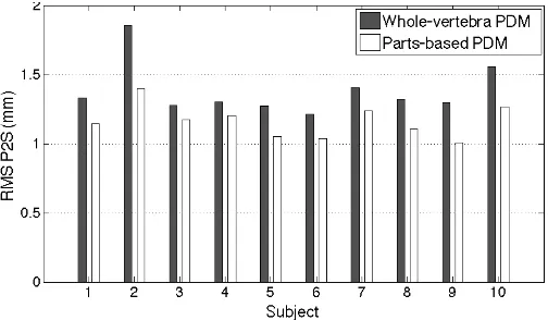
[image:9.612.49.300.127.513.2]We evaluated the performance of our algorithm on the healthy datasets described in section III-A. We performed segmentation on the 30 subjects leaving-one-out both using a whole-vertebra PDM, and our technique.
Fig. 7 shows the segmentation errors for all 30 scans using both ASM methods. It is evident that the proposed technique outperforms the whole-vertebra model ASMs in all cases. The median improvement is of 20% and in some cases the improvement is over 30% due to the ability of the proposed technique to better encode the fine details of the vertebrae.
[image:9.612.317.542.363.498.2]distribution for the whole-vertebra PDM segmentation, and the proposed technique. It can be seen that the errors introduced locally by the use of a whole-vertebra model are corrected by the proposed approach. In both views it is clear that the errors are consistently low in all regions of the vertebra. Also it is evident that the major improvements in accuracy stem from improved fitting of high curvature regions at all processes i.e., spinous, transverse and articular.
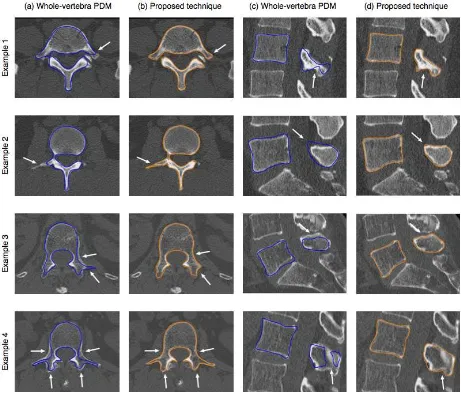
Finally, some examples are given in Fig. 11 to visually illustrate the strength of the proposed technique. The axial views in columns (a) and (b) show how the segmentation using a whole-vertebra PDM (column (a)) can be typically affected in various areas due to the geometrical complexity and high variability involved, as shown by the arrows. In contrast, the proposed technique (column (b)), due to its use of decomposed statistical constraints adapts better to the areas of high geometrical complexity.
Columns (c) and (d) show a sagittal view of the segmenta-tions. It can be seen that both the whole-vertebra PDM and the proposed technique have a similar performance for the main body of the vertebrae, as it is geometrically less complex. On the other hand, the whole-vertebra PDM introduces significant errors in the regions of the processes due their more complex nature as indicated by the arrows. These errors are corrected by the proposed technique.
D. Segmentation Accuracy - Pathological Population
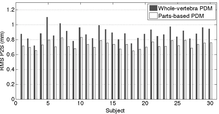
In this section we test whether the technique also improves the segmentation of pathological cases. To this end, we train the statistical models on the population of healthy patients as it is the larger sample providing more class specific variability. Fig. 9 shows the segmentation errors for the 10 pathological scans using both the whole-vertebra ASM and our method. The plot shows that the proposed technique outperforms the whole-vertebra model ASM for all cases. The average improvement is of 17%with the largest improvement at32% for patient 2, and least improvement at8% for patient 4.
It is apparent from the magnitude of the errors that both the whole-vertebra ASM and our technique perform worse on pathological cases as compared to the healthy patients. The error is increased by an average of 36% compared to the healthy patient population. Nonetheless, it can be seen that the relative improvement of the proposed algorithm remains constant. It should be noted that all of the pathological images have a lower resolution along the z-axis which may account for the increased errors, nonetheless, these images also have higher in-plane resolution compared to the healthy images.
Table III summarizes the segmentation results for the whole-vertebra ASM, and the proposed technique for all lumbar vertebrae (L1 to L5). It can be seen that the performance of the proposed technique is consistently better for the entire lumbar spine and particularly for the L3 at 19%. On average, the maximum error was also reduced by 19%, with the highest error reduction for the L2 and L3 at 20%.
a coronal view (columns (a) and (b)), and a sagittal view (columns (c) and (d)) of the same patient. In Example 1 (top), two vertebrae (L2 and L3) are fractured (see white arrows), and it can be seen that the proposed algorithm (columns (b) and (d)) has the flexibility to represent the fracture for both L2 and L3, whereas the whole-vertebra PDM fails to adapt to the contour.
[image:10.612.312.564.247.394.2]Similarly, Example 2 (bottom) shows a fractured L3 ver-tebra (see white arrows). Columns (a) and (c) show how the whole-vertebra PDM does not have the flexibility to fully adapt to the pathological contour while our method (columns (b) and (d)) is able to represent the pathology.
Figure 9. Abnormal population: Point to surface segmentation error compar-ison between the proposed method and the whole-vertebra ASM.
IV. CONCLUSION
Detailed segmentation of the spine is challenged by the geometrical complexity and the high variability of the verte-brae particularly at the processes and in pathological cases. To address this issue, we presented in this paper a novel solution based on a statistical part-based decomposition of the vertebral shape, such that the total variance of the sample population is evenly distributed among the different subregions. Conditional inter-part models are then constructed to maintain the statis-tical coherence of the ensemble of shapes during the model fitting process at the time of image segmentation. In addition, a probabilistic model fitting approach is introduced to robustly select the most likely shape parameters of each subregion.
The obtained segmentation results indicate that our ap-proach can provide highly accurate and consistent segmen-tations throughout different individuals and regions of the vertebra. In particular, the segmentation adapts well to areas that are geometrically complex or highly curved such as the vertebral processes, and to abnormalities such as fractured vertebrae. We also show that the proposed method outperforms the segmentation accuracy obtained with a whole-vertebra PDM.
Figure 7. Normal population: Point to surface segmentation error comparison between the proposed method and the whole-vertebra ASM.
Table II
NORMAL POPULATION: IMAGE SEGMENTATION ERRORS(mm)COMPARING THE PERFORMANCE OF OUR TECHNIQUE AGAINST A WHOLE-VERTEBRA
PDMSEGMENTATION. ERRORS ARE SHOWN INDIVIDUALLY FOR EACH LUMBAR VERTEBRA.
Whole-vertebra PDM (mm) Proposed technique (mm) Improvement (%)
Mean ±Std Max Min Mean ±Std Max Min Mean ±Std Max Min
L1 0.83 0.09 1.12 0.66 0.67 0.06 0.79 0.61 19% 33% 29% 8%
L2 0.84 0.07 1.12 0.64 0.68 0.06 0.83 0.60 19% 14% 26% 6%
L3 0.88 0.09 1.17 0.68 0.71 0.08 0.95 0.60 20% 11% 19% 11%
L4 0.90 0.08 1.15 0.66 0.73 0.06 0.83 0.64 18% 25% 28% 3%
L5 1.02 0.11 1.32 0.82 0.80 0.06 0.89 0.72 22% 45% 33% 12%
All 0.89 0.09 1.18 0.70 0.72 0.07 0.86 0.63 20% 26% 27% 8%
Figure 10. Abnormal population: Comparison of the mean error distribution between the whole-vertebra PDM reconstruction and our part-based PDM reconstruction. Showing lateral and anterior views from left to right, respectively.
[image:12.612.75.536.304.699.2]Table III
ABNORMAL POPULATION: IMAGE SEGMENTATION ERRORS(mm)COMPARING THE PERFORMANCE OF OUR TECHNIQUE AGAINST A WHOLE-VERTEBRA
PDMSEGMENTATION. ERRORS ARE SHOWN INDIVIDUALLY FOR EACH LUMBAR VERTEBRA.
Whole-vertebra PDM (mm) Proposed technique (mm) Improvement (%)
Mean ±Std Max Min Mean ±Std Max Min Mean ±Std Max Min
L1 1.29 0.09 1.41 1.14 1.09 0.05 1.15 0.95 16% 45% 19% 17%
L2 1.37 0.24 2.01 1.17 1.14 0.17 1.62 1.01 17% 30% 20% 14%
L3 1.42 0.13 1.56 1.18 1.16 0.06 1.25 0.99 19% 54% 20% 17%
L4 1.37 0.19 1.81 1.20 1.16 0.13 1.49 1.01 16% 32% 18% 16%
L5 1.47 0.15 1.68 1.27 1.22 0.09 1.41 1.09 18% 40% 17% 15%
All 1.38 0.16 1.69 1.19 1.15 0.10 1.38 1.01 17% 40% 19% 16%
A. Limitations
One limitation of the proposed technique is related to the computational costs that it requires. At training, the statistical decomposition due to its iterative nature is computationally demanding. For 15 subdivisions, for example, the algorithm converges after 6.8 minutes. However, this stage is performed once offline and the conditional models are then saved for image segmentation. At the segmentation stage, the proposed technique is more expensive than the whole-vertebra model segmentation, taking 32 seconds on average per patient (L1 through L5), due to the use of multiple conditional shape models, while the whole-vertebra model segmentation takes 18 seconds to complete the same patient.
A potential challenge of the decomposition approach is that it can theoretically produce discontinuities between two adjacent subparts of the vertebrae. This is because we only use implicit constraints based on the conditional models to obtain a statistical coherence of the ensemble, but this does not guarantee explicitly smoothness between adjacent subregions. In our experimental results, however, we found that these implicit constraints, together with the probabilistic model fitting approach, have a good performance at maintaining the smoothness of the vertebrae, as illustrated in the examples of Figs. 11, and 12. Alternatively, one could consider adding an extra step after the segmentation, where discontinuous transitions between subregions are identified and corrected using smoothing.
B. Future Work
One interesting avenue for future work would be the si-multaneous segmentation of the complete lumbar structure, or larger vertebral groups that include thoracic and/or cervical vertebrae. As it is presented, our algorithm is sequential i.e., it is applied to one vertebra at a time, and all the statistical constraints are within-vertebra constraints. However, we would like to extend the probabilistic framework to include interaction between adjacent vertebral structures assuming shape correlations between them. Considering inter-vertebral relationships would not only account for a more holistic model, but it would also aid in the automatic initialization of most vertebrae thus reducing the human interaction needed for segmentation.
A natural consequence of considering interactions between neighboring structures is then the development of a system of weights to balance the influence of the inter vs. the intra prob-abilistic relationships between the different objects and their constituent subparts. These weights can be shape correlation-driven or image-correlation-driven. We expect to continue work in this direction.
REFERENCES
[1] H.-M. Mayer,Minimally invasive spine surgery. Springer, 2006.
Medical engineering & physics, vol. 30, no. 10, pp. 1287–1304, 2008. [4] A. Middleditch and J. Oliver,Functional anatomy of the spine. Elsevier
Health Sciences, 2005.
[5] H. A. Yuan, S. R. Garfin, C. A. Dickman, and S. M. Mardjetko, “A historical cohort study of pedicle screw fixation in thoracic, lumbar, and sacral spinal fusion,”Spine, vol. 19, no. 20, pp. 2279S–2296S, 1994. [6] L. Hansen, M. De Zee, J. Rasmussen, T. B. Andersen, C. Wong, and
E. B. Simonsen, “Anatomy and biomechanics of the back muscles in the lumbar spine with reference to biomechanical modeling,”Spine, vol. 31, no. 17, pp. 1888–1899, 2006.
[7] S. Benameur, M. Mignotte, S. Parent, H. Labelle, W. Skalli, and J. de Guise, “3D/2D registration and segmentation of scoliotic vertebrae using statistical models,”Computerized Medical Imaging and Graphics, vol. 27, no. 5, pp. 321–337, 2003.
[8] M. G. Roberts, T. F. Cootes, and J. E. Adams, “Linking sequences of active appearance sub-models via constraints: An application in auto-mated vertebral morphometry,” inBritish Machine Vision Conference, 2003, pp. 1–10.
[9] J. Kaminsky, P. Klinge, T. Rodt, M. Bokemeyer, W. Luedemann, and M. Samii, “Specially adapted interactive tools for an improved 3D-segmentation of the spine,” Computerized Medical Imaging and Graphics, vol. 28, no. 3, pp. 119–127, 2004.
[10] M. de Bruijne and M. Nielsen, “Image segmentation by shape particle filtering,” inProc. Int. Conf. on Pattern Recognition, 2004, pp. 722–725. [11] A. Mastmeyer, K. Engelke, C. Fuchs, and W. A. Kalender, “A hierar-chical 3D segmentation method and the definition of vertebral body coordinate systems for QCT of the lumbar spine,” Medical Image Analysis, vol. 10, no. 4, pp. 560–577, 2006.
[12] Z. Peng, J. Zhong, W. Wee, and J.-h. Lee, “Automated vertebra detection and segmentation from the whole spine MR images,” inEngineering in Medicine and Biology Society, 2005. IEEE-EMBS 2005. 27th Annual International Conference of the. IEEE, 2006, pp. 2527–2530. [13] “Learning-based vertebra detection and iterative normalized-cut
seg-mentation for spinal MRI, author=Huang, Szu-Hao and Chu, Yi-Hong and Lai, Shang-Hong and Novak, Carol L, journal=Medical Imag-ing, IEEE Transactions on, volume=28, number=10, pages=1595–1605, year=2009, publisher=IEEE.”
[14] Y. Kim and D. Kim, “A fully automatic vertebra segmentation method using 3D deformable fences,” Computerized Medical Imaging and Graphics, vol. 33, no. 5, pp. 343–352, 2009.
[15] T. Klinder, J. Ostermann, M. Ehm, A. Franz, R. Kneser, and C. Lorenz, “Automated model-based vertebra detection, identification, and segmen-tation in CT images,”Medical image analysis, vol. 13, no. 3, pp. 471– 482, 2009.
[16] J. Ma, L. Lu, Y. Zhan, X. Zhou, M. Salganicoff, and A. Krishnan, “Hierarchical segmentation and identification of thoracic vertebra using learning-based edge detection and coarse-to-fine deformable model,” in Medical Image Computing and Computer-Assisted Intervention– MICCAI 2010. Springer, 2010, pp. 19–27.
[17] D. ˇStern, B. Likar, F. Pernuˇs, and T. Vrtovec, “Parametric modelling and segmentation of vertebral bodies in 3D CT and MR spine images,”
Physics in medicine and biology, vol. 56, no. 23, p. 7505, 2011. [18] A. Rasoulian, R. Rohling, and P. Abolmaesumi, “Lumbar spine
segmen-tation using a statistical multi-vertebrae anatomical shape+pose model,”
Medical Imaging, IEEE Transactions on, vol. 32, no. 10, pp. 1890–1900, Oct 2013.
[19] S. Kadoury, H. Labelle, and N. Paragios, “Spine segmentation in medical images using manifold embeddings and higher-order MRFs,”Medical Imaging, IEEE Transactions on, vol. 32, no. 7, pp. 1227–1238, 2013. [20] J. Huang, F. Jian, H. Wu, and H. Li, “An improved level set method
for vertebra CT image segmentation,” Biomedical engineering online, vol. 12, no. 1, p. 48, 2013.
[21] I. Castro-Mateos, J. M. Pozo, P. E. Eltes, L. Del Rio, A. Lazary, and A. F. Frangi, “3D segmentation of annulus fibrosus and nucleus pulposus from T2-weighted magnetic resonance images,”Physics in Medicine and Biology, vol. 59, no. 24, p. 7847, 2014.
[22] C. Davatzikos, X. Tao, and D. Shen, “Hierarchical active shape models, using the wavelet transform,”Medical Imaging, IEEE Transactions on, vol. 22, pp. 414–423, March 2003.
statistical shape model,” inMedical Image Computing and Computer-Assisted Intervention–MICCAI 2007, N. A. et al., Ed., vol. 4792, 2007, pp. 86–93.
[24] T. Okada, K. Yokota, M. Hori, M. Nakamoto, H. Nakamura, and Y. Sato, “Construction of hierarchical multi-organ statistical atlases and their application to multi-organ segmentation from CT images,” inMedical Image Computing and Computer-Assisted Intervention–MICCAI 2008, D. M. et al., Ed., vol. 5241, 2008, pp. 502–509.
[25] J. Yang, L. H. Staib, and J. S. Duncan, “Neighbor-constrained segmen-tation with level set based 3-D deformable models,”Medical Imaging, IEEE Transactions on, vol. 23, no. 8, pp. 940–948, August 2004. [26] T. Heap and D. Hogg, “Improving specificity in PDMs using a
hierar-chical approach.” inBritish Machine Vision Conference, 1997. [27] T. F. Cootes and C. J. Taylor, “A mixture model for representing shape
variation,”Image and Vision Computing, vol. 17, no. 8, pp. 567–573, 1999.
[28] M. Perea˜nez, K. Lekadir, C. Hoogendoorn, I. Castro-Mateos, and A. Frangi, “Detailed vertebral segmentation using part-based decom-position and conditional shape models,” inRecent Advances in Com-putational Methods and Clinical Applications for Spine Imaging, ser. LNCVB, J. Yao, B. Glocker, T. Klinder, and S. Li, Eds. Springer, 2015, vol. 20, (to appear).
[29] C. Goodall, “Procrustes methods in the statistical analysis of shape,”
Journal of the Royal Statistical Society - Series B: Statistical Method-ology, vol. 53, no. 2, pp. 285–339, 1991.
[30] A. E. Hoerl and R. W. Kennard, “Ridge regression: Biased estimation for nonorthogonal problems,”Technometrics, vol. 12, no. 1, pp. 55–67, 1970.
[31] C. Metz, N. Baka, H. Kirisli, M. Schaap, T. van Walsum, S. Klein, L. Neefjes, N. Mollet, B. Lelieveldt, M. de Bruijneet al., “Conditional shape models for cardiac motion estimation,” inMedical Image Com-puting and Computer-Assisted Intervention–MICCAI 2010. Springer, 2010, pp. 452–459.