A Novel Data Classifier Using Social Spider Optimization

1756 Published By:

A Novel Data Classifier Using

Social Spider Optimization

RavichandranThalamala, B. Janet, A.V. Reddy

Abstract: In current decade, Social Spider Optimization (SSO) has become popular among researchers due to its abilityto represent and handle very high and complex dimensional solution space. Like the other nature inspired algorithms,it also takes inspiration from nature. It mimics the cooperative behavior of social spiders in the forests. Unlike theother nature inspired algorithms, its agents have gender property due to which the algorithm maintains the balancebetween exploration and exploitation. Recently, a few researchers have employed SSO for clustering data. In this article,we propose a new classification algorithm called All Prototypes Social Spider Optimization for Data Classification(APSSODC) in which each spider has the prototypes of all data instances of the dataset. As the dimensionality ofsolution space in APSSODC is very high and equal to the product of degree and cardinality of the dataset, we proposeanother algorithm called Single Prototype Social Spider Optimization for Data Classification (SPSSODC) that reducesthe dimensionality of the solution space. It considers each spider as a single prototype of a data instance present in thedataset. Wefound that SPSSODC outperforms the existing algorithms including APSSODC with respect to classificationaccuracy.

Key words: Nature inspired algorithms, Data classification, Social spider optimization, Solution space, lassificationaccuracy

I. INTRODUCTION

Classification is a data mining approach that is used to identify the class label of given data instance on thebasis of a training data set, in which the class labels of all data instances are known (Alpaydin and Ethem,2010). The algorithm that generates the class of the given data instance is called classifier. Mathematically speaking, a classifier is a mathematical function that maps a given data instance to the label of a class towhich the given data instance belongs to. The application areas of data classification are speech recognition,URL classification, computer vision, drug discovery, biometric identification, e-mail classification, and bank loanapplication processing etc.

Revised Manuscript Received on June 05, 2019 RavichandranThalamala,

B. Janet, A.V. Reddy

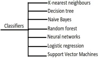
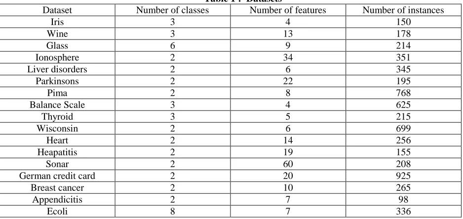
Figure 1: Types of most commonly used classifiers The most commonly used classifiers in machine learning are specified in Figure 1.K-nearest neighbors classifier is a lazy algorithm. After finding out K-neighbors of the given data instance,we determine their classes and assign the given data instance to the class that contains majority of K-neighbors(Indu et al., 2013). Decision tree classifier is one of the most widely used techniques (Katz et al., 2014). Awell de ned set of questions will be asked about the attribute values of the given data instance until the classlabel of the data instance is found (Alexandru and Gabriela, 2017). Naive Bayes classifier assumes that any twoattributes present in a class are independent of each other. After creating frequency table and likelihood table,it uses Naive Bayesian equation to calculate the posterior probability of each class. The data instance belongsto the class having highest posterior probability (Wei and Feng, 2011). Support vector machines classifier represents the training data instances as points in space such that a clear gap is constructed among the data instances of different classes. The class of the given data instance is found based on which side of the clear gap it falls (Seunghee and Jinwook, 2014). Random Forest classifier builds a set of decision trees by taking randomly selected subsets of training data to avoid noise. The class of the given data instance is the class that is predicted by majority of the decision trees (Pall et al., 2006). Logistic regression finds the best fitting model that describes the relationship between independent variables (predictor attributes) and dependent variable (class attribute) by estimating probabilities using logistic function. These probabilities are transformed into binary values to predict the class of the given data instance (Stephan et al., 2002). Neural networks is loosely inspired by the biological neural networks that forms animal brains. A neural network is a collection of interconnected nodes called neurons (Jurgen, 2015). Each neuron has a set of input values, their associated weights and a function that sums the

A Novel Data Classifier Using Social Spider Optimization

input, hidden, and output layers.

Neurons for all possible classes will present in output layer.In this article, we expressed classification as a maximization problem using eqs. (1) and (2). In eq. (2),R is the total number of data instances in the dataset DS, datainstancei is ith data instance in DS , and F is a classification function that takes DS and returns a set CL of classes containing data instances such that the percentage of correctly classified data instances in DS is maximized.

𝐼𝑠𝐶𝑜𝑟𝑟𝑒𝑐𝑡𝐶𝑙𝑎𝑠𝑠 𝑥, 𝐷𝑆

= 1 𝑖𝑓 𝑑𝑎𝑡𝑎 𝑖𝑛𝑠𝑡𝑎𝑛𝑐𝑒 𝑥 𝑖𝑠 𝑐𝑜𝑟𝑟𝑒𝑐𝑡𝑙𝑦 𝑐𝑙𝑎𝑠𝑠𝑖𝑓𝑖𝑒𝑑 𝑛 𝑡𝑕𝑒 𝑑𝑎𝑡𝑎𝑠𝑒𝑡 𝐷𝑆

0 𝑜𝑡𝑕𝑒𝑟𝑤𝑖𝑠𝑒

(1)

𝑀𝑎𝑥 𝐹 𝐷𝑆, 𝐶𝐿 = 𝑅𝑖=1𝐼𝑠𝐶𝑜𝑟𝑟𝑒𝑐𝑡𝐶𝑙 𝑎𝑠𝑠 (𝑑𝑎𝑡𝑎𝑖𝑛𝑠𝑡𝑎𝑛𝑐𝑒 𝑖,𝐷𝑆)

𝑅 ∗

100 (2)

A. Contribution

A lot of research has been done on classification algorithms based on machine learning. Most of these algorithms produce local optimal classification models and some of these algorithms are not suitable to all domains (Saroj et al., 2018). More over, most of the machine learning algorithms use computationally expensive subroutines and tuning learning algorithm

parameters is achieved through multiple executions (V. Bolon-Canedo et al., 2015). So, many researchers have started the study of considering the nature inspired algorithms as alternatives to machine learning algorithms. Some researchers have already used PSO and other nature inspired algorithms in data classification. But they applied their proposed algorithms on low dimensional data sets only.

Some researchers have expressed their concerns about the effectiveness of nature inspired algorithms like PSOwhen applied on high dimensional datasets (Anwar Ali Yahya et al., 2017). They concluded that performanceof nature inspired algorithms like PSO is inversely proportional to the product of the cardinality and degreeof the dataset. More over, there is a possibility of getting local optimum in PSO and other nature inspiredalgorithms.SSO is relatively a new nature inspired algorithm that mimics the cooperative behavior of social spiders(Thalamala et al., 2018a). The male spiders change their positions in small steps based on the vibrations fromnearest female spider. The female spiders receive the vibrations from the globally best spider and nearest betterspider to change their positions in the solution space with relatively bigger steps (Thalamala et al., 2017). It hasbeen already shown that SSO can be used for clustering of data and produces better clustering results than othernature inspired algorithms (Thalamala et al., 2018b). In this article, we proposed two classification algorithmsbased on SSO. We applied them on both low and high

dimensional datasets, and found better

classificationaccuracy. We selected SSO for data classification due to below reasons.Randomness plays very important role in SSO. It is used in initializing the spiders and changing theirpositions. If the randomness is produced in a systematic way, the solution space can be explored efficiently. Inour proposed algorithms, we used logistic

chaotic map function to achieve systematic

randomness.Each dominant male spider in SSO participates in mating with a set of female spiders to produce a newspider. If the weight of the new spider is greater than that of the worst spider, the worst spider will be replacedby the new spider. But there is no guarantee that the weight of each new spider is greater than the weight ofthe worst spider. In other words, there is no guarantee that each mating operation leads to a better solutionspace. To avoid this problem, we allowed only the dominant male spiders whose weight is greater than or equalto the average weight of them to participate in the mating operation. Each of these

dominant male spiders willproduce a new spider whose weight is greater than that of the worst spider. The structure of this article is as follows. Section 2 briefly specifies the related work on data classificationusing nature inspired algorithms. Section 3 describes the two proposed algorithms. Section 4 includes andexplains the experimental results of the proposed work, and the conclusion is specified in section 5.

II. RELATED WORK

(De Falco I et al., 2007) defined three fitness functions for classification using Particle swarm optimization(PSO). The firstfitness function returns the percentage of incorrectly assigned data instances in the dataset. The second one returns the sum of Euclidean distances of the data instances from their centroids. The third oneis a linear combination of the first two. The better version of PSO, in fact, the third version of PSO is comparedwith other classification techniques. They showed that PSO occupies the fourth position in the ranking basedon classification accuracy. They also showed that PSO is the best for three out of five binary classificationproblems.

(Qi et al., 2008) hybridized PSO with tabu search (TS) for tumor classification.They showed that the hybrid algorithm produces better resultsthan the TS algorithm and PSO algorithm when applied on micro array datasets.

(Alejandro et al., 2009) proposed Standard PSO and

adaptive Michigan PSO (AMPSO) for

Continuousclassification problems. In Standard PSO, each particle is a collection of all prototypes in the solution space.So, the number of dimensions of the solution space is very high. AMPSO reduces the dimensionality of thesolution space and provides higher classification accuracy by representing each particle as a prototype in thesolution space. The algorithm returns the entire swarm as the solution to the problem. They compared theresults of the standard PSO and AMPSO and found that AMPSO always produces a better solution than thestandard PSO. They also found that AMPSO can improve the classification accuracy of the Nearest Neighborclassifiers. (P. Shanmugapriya et al., 2012)

applied Ant Colony

1758 Published By: the classification accuracy gradually increases as

pheromoneevaporation rate (PER) is increased up to 0.75 and decreases when PER exceeds 0.75.

(Mauricio Schiezaro et al., 2013) used Artificial Bee Colony (ABC) algorithm to improve classificationaccuracy by reducing the number of selected features in the datasets. They showed that the classificationaccuracy significantly increases as the number of selected features decreases. Besides that, they showed thatABC produces superior results for most of the datasets when compared to PSO, Ant Colony Optimization(ACO) and Genetic algorithms (GA). (Fernando E. B. Otero et al., 2013) proposed a new effective search method to find the list of classificationrules using ACO algorithm. The search performed by ACO depends on the quality of a candidate list of rules.The sequence in which the classification rules should be created is specified in the pheromone matrix . Theycompared the classification results of the proposed algorithm with other state-of-the-art algorithms and foundthat the proposed algorithm is the most accurate algorithm.

(J. Jayanth et al., 2015) applied ABC algorithm for classifying remote sensing data of spatial images.Each image is associated with a Digital Number (DN) and each class of images is associated with a rangeof DN values. They showed that ABC produces better classification accuracy than Artificial Neural Network(ANN), Support Vector Machine (SVM), and Maximum Likelihood Classifier (MLC) by effectively handlingand correlation issues.

(Mohammed Alweshah et al., 2015) proposed two classification algorithms, namely firefly algorithm with simulated annealing for probabilistic neural network (SFA-PNN) and firefly algorithm with levy light for theprobabilistic neural network (LFA-PNN) that hybridize FA (firefly algorithm) with simulated annealing andlevy light respectively in order to improve the efficiency of the PNN. They proposed another classificationalgorithm, namely SFA with levy light for the probabilistic neural network (LSFA-PNN) that integrates theSFA with levylight in order to get more improvement in the efficiency of the PNN. As these hybrid versionsmaintain the balance between exploration and exploitation, they produced better classification results thanFirefly algorithm for the PNN ( FA-PNN). Among these hybrids, LSFA produced the best classification resultsas it is capable of controlling random walk in FA.

(JanmenjoyNayak et al., 2016) proposed a a classification algorithm, namely firefly algorithm for Pi-sigma neural networks (FFA-PSNN) that combines firefly algorithm with the Pi-sigma neural networks in orderto get better classification accuracy. Each firefly in the solution space represents a weight set of PSNN. Theproposed algorithm returns the optimal weights of PSNN. They comparedthe classification accuracy of FFA-PSNN with Genetic algorithms for Pi-sigma neural networks (GA-PSNN),Particle swarm optimization for Pi-sigma neural networks (PSO-PSNN) and hybrid GA-PSO for Pi-sigma neural networks (GA-PSO-PSNN).

(Saroj et al., 2018) proposed a framework for fitness computation that can be used with any nature inspired algorithm. The performance of a classification rule can be computed using this fitness function. A confusion table that specifies the number of true positives (TP), number of true negatives (TN), number of false positives (FP), and number of false negatives (FN) is constructed using training data. Then precision is computed as the ratio of T P and (T P +F P ), whereas the recall is computed as the ratio of T P and (T P +F N). They defined the fitness of the classification rule as the product of precision and recall. They proved that the proposed framework is very efficient as compared to

finding fitness through scanning of database. They used a genetic algorithm for finding out classification rules. (Binh, et al., 2018) proposed a new algorithm called potential particle swarm optimization for dimensionality reduction. They employed a new representation for particles. Each particle is an integer vector whose size is equal to the number of the original features. The potential cut points of each feature are stored in a potential cut point table. The dimension of the particle should be in between 1 and the number of potential cut points of the corresponding feature. They showed that the proposed algorithm reduces the dimensionality better than other algorithms. They also showed that the classification accuracy of Naive bayes algorithm can be improved with the help of the proposed algorithm.

(Hala et al., 2018) hybridized correlation based feature selection method (CFS) and ABC for increasing classification accuracy of gene expression pro le. The proposed algorithm has three cooperative phases. In first phase, CFS projects over the subset of feature set that has maximal correlation to the class and minimal correlation between features in it, and filters noisy and redundant genes. In second phase, the genes that are informative and meaningful are found. In third phase, SVM is used as a classifier on selected genes from the second phase. The results show that the proposed algorithm has better classification accuracy than the other algorithms.

III. METHODS

A. SSO

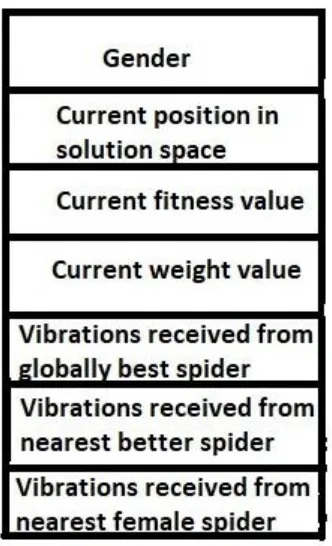
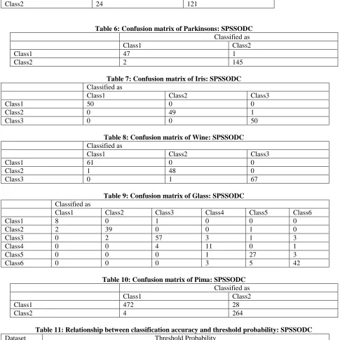
The standard SSO initiates the spiders and moves them in the real valued multi dimensional solution space. Afemale spider moves in the solution space based on the vibrations received from the globally best spider andnearest better spider (Erik et al., 2013). Threshold probability (TP) plays an important role in determiningthe next positions of female spiders (Ruxin et al., 2017). If it is greater than generated random value, thefemale spiders change their positions to attract the globally best spider and nearest better spiders of them.Otherwise, they repulse the globally best spider and nearest better spiders and move away from them. Thedominant male spiders change their positions with respect to the nearest female spider. Because of their high fitness, they mate with a set of female spiders to produce a new spider. As the worst spiders hardly have fitness, they can be replaced with the newly generated spiders that have more fitness (Erik et al., 2016). The male spiders that have fitness less than the median fitness of male spiders are called non dominant spiders (Zhou et al., 2017). The next position of a non-dominant male spider depends on all male spiders present in the search space. The representation of a spider in SSO is as shown in Figure 2. Each spider possesses a gender value, its current position in the solution space, its current fitness, its current weight, and a set of vibrations received from the globally best spider, its nearest better spider and its nearest female spider. The vibrations received by spider si from spider sj can be calculated using eq. (3). In

eq. (3), weight[j]

A Novel Data Classifier Using Social Spider Optimization

represents the distance between spider si and spider sj. In eq. (3), vibrations[i, j] represents the vibrations received by spider si from spider sj .

𝑣𝑖𝑏𝑟𝑎𝑡𝑖𝑜𝑛𝑠 𝑖, 𝑗 = 𝑤𝑒𝑖𝑔𝑕𝑡 𝑗 ∗ 𝑒−𝑑𝑖𝑠𝑡𝑎𝑛𝑐𝑒 (𝑖,𝑗 )2

(3)

Figure 2: Representation of a spider in SSO

B. APSSODC

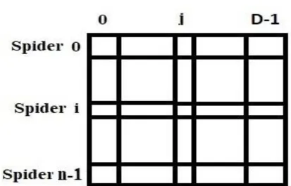
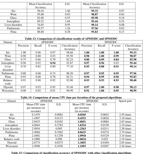
Let R be the number of data instances in the dataset and D be the number of dimensions in each data instance. In APSSODC, each spider is a collection of R prototypes, and

each prototype has D dimensions as shown in Figure3. Besides these prototypes, each spider maintains a list of data instances correctly classified by it and their corresponding classes.Algorithm2 specifies the steps in APSSODC. Algorithm 1: Fitness of spider in APSSODC

INPUT: s : spider

OUTPUT: tness[s] :tness of spider s procedure Fitness()

CClass = 0

for each data instance i in the dataset DS do Find the nearest prototype p in spider s

if class(i) = class(p) then CClass = (CClass + 1)

Add data instance i and class(i) to the spider s end if

end for

fitness[s]= CClass ÷ R

1760 Published By: Figure 3: APSSODC: Representation of spiders

A Novel Data Classifier Using Social Spider Optimization

Algorithm 2: All Prototypes Social Spider Optimization : APSSODC

INPUTS: DS : Dataset, S : population size, M AXITER : Maximum number of iterations,

PF :Threshold Probability

OUTPUTS: gbs : Globally best spider, fitness[gbs] : Classification accuracy of Globally best spider

procedure APSSODC()

1: Take the number of females F as 70-90% of S randomly

2: Compute the number of males M= S - F 3: for each spider s in the population do

4: Initialize all dimensions of all prototypes of s randomly using eq. (4)

5: end for 6: Set iter to 1

7: while iter<= M AXIT ER do

8: for each spider s in the population do 9: Call Fitness(s)

10: Find weight[s] using eq. (5) 11: end for

12: update globally best spider gbs

13: for each female spiders in the population do

14: Generate a random number r 15: if r < T P then

16: Update all dimensions of all prototypes of s randomly using eq. (6)

17: else

18: Update all dimensions of all prototypes of s randomly using eq. (7)

19: end if 20: end for

21: for each male spider s in the population do 22: if s is a dominant male then

23: Update all dimensions of all prototypes of s randomly using eq. (8)

24: else

25: Update all dimensions of all prototypes of s randomly using eq. (9)

26: end if 27: end for 28: Call Mating 29: Increment iter by 1 30: end while

31: Return gbs, and fitness[gbs] as its classification accuracy

end procedure

Algorithm 3: Mating procedure Mating()

1: for each dominant male spider s whose weight is greater than or equal to average weight of dominant male spiders do

2: Find the set of females F , with in the radius of mating

3: if F is empty then 4: continue 5: end if

6: Generate new spider ns using eq. (10) 7: Replace worst spider with new spider 8: end for

end procedure

1) Initialization of Spiders

During the initialization process, each dimension of prototypes of each spider is initialized with a random numberin between its lower bound and upper bound. The random numbers are generated using logistic chaotic map function. spider[i, j, k] that represents kth dimension of jth prototype of spider i is initialized using eq. (4). In eq. (4), minimum(k) and maximum(k) represent the smallest and largest values of kth dimension of the datasetrespectively.

𝑠𝑝𝑖𝑑𝑒𝑟 𝑖, 𝑗, 𝑘 = 𝑚𝑖𝑛𝑖𝑚𝑢𝑚 𝑘 + 𝑟𝑎𝑛𝑑𝑜𝑚 0, 1 ∗ (𝑚𝑎𝑥𝑖𝑚𝑢𝑚 𝑘 − 𝑚𝑖𝑛𝑖𝑚𝑢𝑚 𝑘 )

(4)

Then the classes of the prototypes of each spider are initialized randomly from 0 to K-1, and the list of correctly classified data instances is set to empty in each spider.

2) Evaluation of Fitness and Weight Values of Each Spider

After the initialization phase is over, the fitness of each spider s is found. The fitness of a spider s specifieshow well it can classify the data instances in the data set. Its value will be in the interval [0, 1]. If the spiders classifies all the data instances correctly, its fitness becomes 1. If it correctly classifies some data instances,its fitness will be greater than 0 and less than 1. Its fitness becomes 0, when it correctly classifies no datainstances. Algorithm1 can be used to find the fitness of a spider s. In that, CClass represents the number ofdata instances which are correctly classified by the spider s. For each data instance in the dataset, the nearestprototype in the spider s

1762 Published By: and its class are added to spider s. The ratio of the

number of data instances added to the spider sand the total number of data instances in the dataset indicates the classification accuracy as well as the fitnessvalue of spider s. The same process is repeated for all the spiders in the population. Having found the fitnessvalues of all spiders, the weight of each spider s is computed using eq. (5).

𝑤𝑒𝑖𝑔𝑕𝑡 𝑠 = 𝑓𝑖𝑡𝑛𝑒𝑠𝑠 𝑠 −𝑓𝑖𝑡𝑛𝑒 𝑠𝑠(𝑆𝑤𝑠)

𝑓𝑖𝑡𝑛𝑒𝑠𝑠 𝑆𝑔𝑏𝑠 −𝑓𝑖𝑡𝑛𝑒𝑠𝑠 (𝑆𝑤𝑠)

(5)

wheresws and sgbs are the worst spider and the globally best spider in the population respectively.

3) Movement of Spiders in Solution Space

At the beginning of each iteration for the movement of spiders, the list of correctly classified data instances ineach spider is set to empty. But the position of the spider in the solution space will not be changed. Each femalespider gets attracted by globally best spider and nearest better spider, or repulsed by them. To implement thetwo basic operations namely attraction and repulsion of female spiders, a random number is generated. If it is less than T P , the female spider is allowed to attract globally best spider and nearest better spider and itsposition will be updated using eq. (6). Otherwise, it is allowed to repulse the two spiders and go away from them using eq. (7).

𝑠𝑝𝑖𝑑𝑒𝑟 𝑖, 𝑗, 𝑘 = 𝑠𝑝𝑖𝑑𝑒𝑟 𝑖, 𝑗, 𝑘 + 𝛼 ∗

𝑠𝑝𝑖𝑑𝑒𝑟 𝑖, 𝑗, 𝑘 − 𝑠𝑝𝑖𝑑𝑒𝑟 𝑔𝑏𝑠, 𝑗, 𝑘 ∗

𝑤𝑒𝑖𝑔𝑕𝑡 𝑔𝑏𝑠 ∗ 𝑒

+ 𝛽 ∗

𝑠𝑝𝑖𝑑𝑒𝑟 𝑖, 𝑗, 𝑘 − 𝑠𝑝𝑖𝑑𝑒𝑟 𝑛𝑏𝑠, 𝑗, 𝑘 ∗

𝑤𝑒𝑖𝑔𝑕𝑡 𝑛𝑏𝑠 ∗ 𝑒

_{+ 𝛾 ∗ (𝛿 −}

0.5)

(6)

𝑠𝑝𝑖𝑑𝑒𝑟 𝑖, 𝑗, 𝑘 = 𝑠𝑝𝑖𝑑𝑒𝑟 𝑖, 𝑗, 𝑘 − 𝛼 ∗

𝑠𝑝𝑖𝑑𝑒𝑟 𝑖, 𝑗, 𝑘 − 𝑠𝑝𝑖𝑑𝑒𝑟 𝑔𝑏𝑠, 𝑗, 𝑘 ∗

𝑤𝑒𝑖𝑔𝑕𝑡 𝑔𝑏𝑠 ∗ 𝑒

− 𝛽 ∗

𝑠𝑝𝑖𝑑𝑒𝑟 𝑖, 𝑗, 𝑘 − 𝑠𝑝𝑖𝑑𝑒𝑟 𝑛𝑏𝑠, 𝑗, 𝑘 ∗

𝑤𝑒𝑖𝑔𝑕𝑡 𝑛𝑏𝑠 ∗ 𝑒

+ 𝛾 ∗ (𝛿 −

0.5

(7)

In eqs. (6) and (7), spider[i,j,k], spider[gbs,j,k] and spider[nbs,j,k] represent real values that specifythe positions of jth prototypes of female spider i, globally best spider (gbs), and nearest better spider (nbs)of i, in kth dimension of the solution space respectively, distance(i, gbs) and distance(i, nbs) are the Euclidean distances of female spider i from gbs, and its nbs respectively, and weight[gbs] and weight[nbs] are weights ofgbs, andnbsrespectively. The dominant male spiders will generally be attracted by nearest

female spiders.As their fitness is greater than median fitness of male spiders, they capture vibrations from the nearest femalespider and move towards it. Its next position can be calculated using eq. (8).

𝑠𝑝𝑖𝑑𝑒𝑟 𝑖, 𝑗, 𝑘 = 𝑠𝑝𝑖𝑑𝑒𝑟 𝑖, 𝑗, 𝑘 + 𝛼 ∗

𝑠𝑝𝑖𝑑𝑒𝑟 𝑖, 𝑗, 𝑘 − 𝑠𝑝𝑖𝑑𝑒𝑟[𝑛𝑓𝑠, 𝑗, 𝑘] ∗

𝑤𝑒𝑖𝑔𝑕𝑡 𝑛𝑓𝑠 ∗ 𝑒

+ 𝛾 ∗ (𝛿 −

0.5)

(8)

In eq. (8), spider[i,j,k] and spider[nfs,j,k] represent real values that specify the positions of jth prototypesof dominant male spider i, and nearest female spider (nfs) of spider i, in kth dimension of the solution spacerespectively,

distance(i,nfs) is the Euclidean distance of dominant male spider i from nfs, and weight[nfs] isthe weight of nfs. The non dominant male spiders change their positions according to eq. (9).

𝑠𝑝𝑖𝑑𝑒𝑟 𝑖, 𝑗, 𝑘 = 𝑠𝑝𝑖𝑑𝑒𝑟 𝑖, 𝑗, 𝑘 + 𝛼 ∗ 𝑊

(9)

In eq. (9), spider[i,j,k] represents a real value that specifies the position of jth prototype of non dominantmale spider i in kth dimension of the solution space, and W is the weighted mean of male population.In theabove eqs. (6), (7) ,(8), and (9), α, β, γ, and δ are random numbers from the interval [0,1].These randomnumbers are generated using logistic chaotic map.

4) Mating of Dominant Male Spiders

Each dominant male spider searches for female spiders present in the range of mating. The range of matingis the ratio of the sum of the differences between maximum and minimum values present in each dimension,and twice the number of dimensions of the solution space.Algorithm3

specifiesthestepsinthematingoperation. The value of range of mating is the same for each dominant male spider. A dominant male spider will not participate in the mating operation, if range of matingcontains no female spiders. In the proposed two algorithms, we allow only the dominant male spiders whoseweight is greater than or equal to average weight of them to mate with the female spiders in order to improve thesolution space. The mating produces a new spider ns whose kth dimension in jth prototype can be found using eq. (10). Then the worst spider will be replaced by new spider and the gender of it is assigned to new spider.

𝑠𝑝𝑖𝑑𝑒𝑟 𝑛𝑠, 𝑗, 𝑘 = 𝑆−1𝑖=0𝑤𝑒𝑖𝑔𝑕𝑡 𝑖 ∗ 𝑠𝑝𝑖𝑑𝑒𝑟[𝑖, 𝑗, 𝑘] 𝑤𝑒𝑖𝑔𝑕𝑡[𝑖] 𝑆−1

𝑖=0

A Novel Data Classifier Using Social Spider Optimization

1763 Published By: C.SPSSODC

As the dimensionality of the solution space is high in APSSODC, we propose SPSSODC in which each spiderrepresents a single prototype consisting of D dimensions as shown in the Figure 4. Besides this prototype,each spider maintains a list of data instances correctly classified by it and their corresponding classes. At thebeginning of each iteration for the movement of spiders, this list is set to empty as in APSSODC. The solutionspace will have as many spiders as the number

of data instances in the dataset. Fitness of each spider s canbe found using Algorithm4. Its possible values are 0 and 1. Initially, the fitness of each spider is set to 0. Itchanges to 1, when the following conditions are satisfied.

 It has the closest prototype of any one of data instances in the data set

 The classes of the prototype and the data

instance are the same

Algorithm 4: Fitness of spider in SPSSODC INPUT: s : spider

OUTPUT: fitness[s]:fitness of spider s

procedure Fitness() 1: fitness[s]=0

2: Find the nearest data instance i in the dataset DS from the prototype p in spider s

3: if class(i) = class(p) then 4: fitness[s]=1

5: Add data instance i and class(i) to the spider s 6: end if

7: Return fitness[s] end procedure

In each iteration, all spiders whose fitness is not equal to one are moved to their next positions based ontheir gender. But the spiders whose fitness is already one remain at the same position in subsequent iterations.After all iterations are over, SPSSODC returns all spiders whose fitness is equal to 1. The classification accuracy is found using eq. (11).

𝐴𝑐𝑐𝑢𝑟𝑎𝑐𝑦 = 𝑛𝑓𝑖𝑡 1

𝑅 ∗ 100 (11)

where𝑛_{𝑓𝑖𝑡1}is the number of spiders whose fitness is equal to 1 in SPSSODC, and R is the number of datainstances in the dataset.

IV. RESULTS

The proposed algorithms are evaluated by carrying out experiments using datasets taken from UCI machine learning repository (M. Lickman, 2013). Table 1 specifies the number of classes, the number of features and the number of data instances present in the datasets used in the experiments. We implemented the two proposed algorithms using Java run time environment of version 1.7.0.51 and Windows 7 Professional operating system on Intel (R) Xeon (R) CPU E3-1270 v3 @ 3.50GHz 3.50GHz processor having RAM of 160 GB capacity. In both proposed algorithms, the number of spiders is set to 50, the maximum number of iterations is set to 1000, and threshold probability is set to 0.7.

A. State-of-art Classification Algorithms

1) Firefly algorithm for PNN (FA-PNN):

PNN is a neural network model that is based on the gradient steepest descent method for solving classification problems. It reduces classification errors by allowing network to correct the network weights (Mohammed Alweshah et al., 2015). FA is an optimization technique in which the rhythmic flashing lights produced by fireflies are considered as the possible solutions. The brightness of flashing light represents the quality of the solution given by it. In FA-PNN, FA is called to find the optimal weights for the network so that the classification accuracy can be improved.

2) Firefly algorithm with simulated annealing for PNN (SFA-PNN):

Like FA-PNN, it uses FA to find optimal weights of PNN. The best solution given by FA is passed to Simulated annealing (SA) to generate a neighbour solution. The new solution will be accepted if it is better than the current best solution or it satisfies the probability rule. If it is not accepted, itsneighbour solution is generated. This process is repeated until temperature becomes equal to zero. Then the best solution produced by SA is passed back to FA. In other words, FA is the improvement algorithm for PNN and SA is the improvement algorithm for FA.

3) Firefly algorithm with levy flight for PNN (LFA-PNN):

Like FA-PNN and SFA-PNN, it also uses FA to find optimal weights of PNN. In FA, the next position of each firefly is effected by a random variable. So, to control exploration produced by random variable and to introduce exploitation, levy flight is introduced.

4) SFA with levy flight for PNN (LSFA-PNN):

It combines levy flight with SFA to control randomness. It gets more balance between exploration and exploitation with the help of levy flight. The length of search space around the current position of a firefly is very large at initial iterations, which leads to exploration. But it decreases gradually as the number of iterations increases, which leads to exploitation.

5) Firefly algorithm for Pi-sigma neural networks (FFA-PSNN):

1764 Retrieval NumberH6600068819 /19©BEIESP

Published By:

Blue Eyes Intelligence Engineering & of tunable weights (JanmenjoyNayak et al., 2016). Firefly

algorithm (FFA) is used to find the optimal weights for PSNN. The number of fireflies is initialized randomly. The fitness of each firefly is computed as the reciprocal of sum of the root mean square error obtained from each data instance of the dataset.

6) Genetic algorithms for Pi-sigma neural networks (GA-PSNN):

GA is used to find the optimal weights of PSNN. It allows the survival of the fittest chromosomes. More over, it has controllable parameters like population size, mutation rate and cross over (D. E. Goldberg, 1989).

7) PSO for Pi-sigma neural networks (PSO-PSNN):

PSO is used to find the optimal weights of PSNN as it has less computational complexity.

8) Hybrid PSO-GA for Pi-sigma neural networks (PSO-GA-PSNN):

As PSO suffers from premature convergence, it is combined with GA in order to find optimal weights of PSNN.

9) CN2 algorithm:

The CN2 induction algorithm is a learning algorithm which is capable of producing production rules even though the given dataset suffers from noise. It is regarded as the combination of both IterativeDichotomizer (ID3) and Algorithm Quasi-optimal (AQ).

10) C4.5 rules:

It is an improved version on ID3. continuous and discrete features. It can produce production rules though the dataset has incomplete data points and solve over-fitting problem.

11) J48:

It is also one of the improved versions on ID3. It is capable of handling missing values. It supports decision tree pruning, continuous attribute value ranges, and derivation of rules.

12) Naive Bayes:

Naive Bayes is a set of probabilistic algorithms based on probability theory and Bayes’ Theorem to predict the tag of a text. Using prior knowledge of conditions related to each feature, Bayes’ Theorem measures the probabilities of them.

13) Sequential minimal optimization (SMO):

It solves the quadratic programming (QP) problem that bubbles up when we conduct training phase of the support vector machines. It converts QP problem into a series of smallest possible sub-problems than can be solved analytically.

14) JRIP:

In JRIP, classes are organized in the increasing order of size. At each iteration, the class at the top of the list is taken out and a set of rules that cover all the members of that class is found. The process is repeated until the list becomes empty.

15) PART:

At each iteration, it constructs a partial C 4.5 decision tree and converts the best leaf into a rule. It uses both divide-and-conquer and separate-divide-and-conquer strategies of rule learning.

16) Pittsburgh PSO (PPSO):

It is based on Particle Swarm Optimization (PSO). Each particle is a candidate solution for the classification problem. Each particle is a collection of $R$ prototypes. The algorithm returns best particle having highest accuracy.

17) Michigan PSO (MPSO):Unlike PPSO, it considers each particle in PSO as a single prototype to reduce the dimensionality of the solution space. The entire swarm is a solution to the classification problem.

18) Adaptive MPSO (AMPSO):

Like MPSO, it considers each particle in PSO as a single prototype. But the population size is not fixed. The number of prototypes and the number of classes of the prototypes may be increased based on certain conditions.

19) PSO + ACO2:

It is a hybrid of PSO and Ant Colony Optimization (ACO) for generating classification rules. It has two steps in the rule construction process. It creates antecedent of a rule using nominal attributes and extends it using continuous attributes.

20) CAnt-Miner2MDL:

It is a variation of the Ant-Miner algorithm. It is based on minimum description length (MDL) principle. It dynamically creates thresholds on the domains of continuous attributes.

21) CAnt-MinerPB:

In this algorithm, each ant creates a complete list of rules at each iteration of the algorithm instead of a single rule and the search is guided by the quality of a list of rules.

B. Classification Results of APSSODC and SPSSODC

Table 2 and Table 3 specify the relationship between the classification accuracy and the number of iterations in both proposed algorithms. The two algorithms are executed 20 times and the mean classification accuracy and standard deviation values are also specified in Table 2 and Table 3. As we increase the number of iterations, the following will happen leading to higher classification accuracy.

 the chance of spiders moving toward locally better position will increase

 the chance of spiders moving toward globally best position will increase

 The chance of exhaustive

exploration of the solution space will increase

A Novel Data Classifier Using Social Spider Optimization

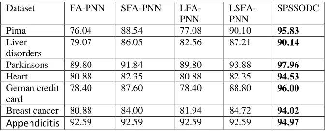
Figure 5: SPSSODC: Ionosphere dataset: the relationship between iterations and correctly classified data instances

1766 Published By: Figure 5 specifies the relationship between iterations and

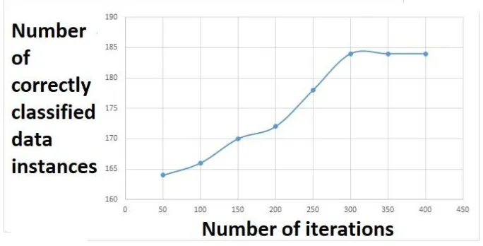
correctly classified data instances when SPSSODC is applied on Ionosphere data set. At 50 iterations, the number of correctly classified data instances is 308 only. As we increase number of iterations to 100, 150, 200, 250 and 300, the number of correctly classified data instances increases to 314, 320, 326, 328 and 335 respectively. After 300 iterations, the number of correctly classified data instances remains at 335 only. Figure 6 specifies the relationship

between iterations and correctly classified data instances when SPSSODC is applied on Wine data set. At 50 iterations, the number of correctly classified data instances is 164 only. As we increase number of iterations to 100, 150, 200, 250 and 300, the number of correctly classified data instances increases to 164, 166, 170, 172, 178 and 184 respectively. After 300 iterations, the number of correctly classified data instances remains at 184 only.

Tables 4-10 indicate confusion matrices of Ionosphere, Liver disorders, Parkinsons, Iris, Glass, and Pima datasets respectively with respect to SPSSODC algorithm. The total of primary diagonal elements in each confusion matrix indicates the total number of correctly classified data instances.

As shown in the confusion matrix of Ionosphere in Table 4, out of 225 data instances of class1, only 216 data instances are correctly classified to class1, the remaining 9 data instances are wrongly classified to class 2. But among 126 data instances of class 2, 119 are correctly classified to class 2 and the remaining 7 data instances are wrongly classified to class 1. As shown in the confusion matrix of Liver disorders in Table 5, out of 200 data instances of class 1, only 190 data instances are correctly classified to class 1, the remaining 10 data instances are wrongly classified to class 2. But among 145 data instances of class 2, 121 are correctly classified to class 2 and the remaining 24 data instances are wrongly classified to class 1. As shown in the confusion matrix of Parkinsions dataset in Table 6, out of 48 data instances of class 1, only 47 data instances are correctly classified to class 1, the remaining 1 data instance is wrongly classified to class 2. But among 147 data instances of class 2, 145 are correctly classified to class 2, and the remaining 2 data instances are wrongly classified to class 1. As shown in the confusion matrix of Iris dataset in Table 7, all 50 instances of both class 1 and class 3 are correctly classified. But among 50 instances of class 2, 49 data instances are correctly classified and one data instance is wrongly classified to class 3. As shown in the confusion matrix of Wine dataset in Table 8, all 61 data instances of class 1 are correctly classified.Out of 49 data instances of class 2, 48 data instances are correctly classified to class 2 and one data instance is wrongly classified to class 1. Among 68 data instances of class 3, one data instance is wrongly classified to class 3.

As shown in the confusion matrix of Glass dataset in Table 9, 1 out of 9 data instances of class 1 is misclassified to class 3. Out of 42 data instances of class 2, 2 data instances are misclassified to class 1 and 1 data instance is misclassified to class 5. Out of 66 data instances of class 3, 2 data instances are misclassified to class 2, 3 data instances are misclassified to class 4, 1 data instances is misclassified to class 5 and 3 data instances are misclassified to class 6. Out of 16 data instances of class 4, 4 data instances are misclassified to class 3 and 1 data instance is misclassified to class 6. Out of 31 data instances of class 5, 3 data instances are misclassified to class 6 and 1 data instance is misclassified to class 4. Out of 50 data instances of class 6, 3 data instances are misclassified to class 4 and 5 data instances are

misclassified to class 5. As shown in the confusion matrix of Pima dataset in Table 10, out of 500 data instances of class 1, only 472 data instances are correctly classified to class 1, the remaining 28 data instances are wrongly classified to class 2. But among 268 data instances of class 2, 264 are correctly classified to class 2 and the remaining 4 data instances are wrongly classified to class 1.

1) Effect of Parameters on Classification Accuracy The movement of female spiders in the solution space depends on Threshold Probability (TP). As shown in Table 11, the mean classification accuracy increases as we increase TP up to 0.7. When TPis equal to 0.7, the best mean classification accuracy is produced. But, when TP is further increased up to 1, the mean classification accuracy gradually decreases. The reason is that when TP value goes closer to 1, the female spiders will be able to perform only attraction operation. As they can notperform repulsion operation, some part of the solution space becomes unexplored. The movement of spiders in the solution space depends on random numbers also. We used logistic chaotic map to produce random numbers. Table 12 shows mean classification accuracy values produced by SPSSODC with and without logistic chaotic map function. We found that SPSSODC using logistic chaotic map function produces better mean classification values due to the systematic randomness provided by the chaotic map.

C. Comparison of Classification Algorithms

Table 13 shows that SPSSODC produces the better classification results than APSSODC with respect to almost all datasets. In addition to the classification accuracy, precision, recall, and F-score are also specified. SPSSODC produces the lowest percentage increase in classification accuracy (i.e. 0.68%) when applied on Iris dataset. The highest percentage increase in classification accuracy (i.e. 16.43%) is produced when it is applied on Pima dataset. The overall percentage increase in classification accuracy is approximately 4%. In case of Ionosphere dataset, APSSODC produces slightly better F-score value than SPSSODC.

The execution time of a classification algorithm depends upon the cardinality of the dataset, the degree of the dataset, the number of classes present in the dataset, and the convergence speed of the

algorithm. We have

A Novel Data Classifier Using Social Spider Optimization

14 shows the mean CPU time per iteration( in seconds) taken by APSSODC and SPSSODC. The speed gained by SPSSODC is also specified. The speed gain is obtained by dividing the CPU time per iteration of APSSODC with that of SPSSODC.

In Table 15, SPSSODC is compared with PPSO, MPSO, AMPSO, J48, PART, Naive Bayes and SMO with respect to classification accuracy. SPSSODC produces the best accuracy for Iris, Liver disorders, Balance Scale, Pima, Thyroid and Winconsin datasets. For Glass dataset, It produces second best accuracy (i.e. 85.98) which is marginally smaller than the accuracy produced by AMPSO. We found that the overall percentage increase in classification accuracy produced by SPSSODC is approximately 12%. The classification results of PPSO, MPSO, AMPSO, J48, PART, Naive Bayes and SMO are taken from (Alejandro et al., 2009). In PPSO, the population size is set to 60, the maximum number of iterations is set to 300, constriction factor value is set to 0.72984, and constant weight factors are set to 2.05. In both MPSO and AMPSO, the population size is set to 60, the maximum number of iterations is set to 300, constriction factor value is set to 0.5, constant weight factors are set to 1.0, 1.0 and 0.25 respectively, and inertia coefficient value is set to 0.1. The parameter 𝑃_𝑟 to tune the probability of reproduction in AMPSO is set to 0.1. For the remaining algorithms, (Alejandro et al., 2009) used the default values proposed by their correspondent authors.

In Table 16, SPSSODC is compared with other classification algorithms with respect to classification accuracy. SPSSODC produces the best accuracy for Iris, Glass, Wine, Ionosphere, Liver disorders, Parkinsons, and Pima datasets. We found that the overallpercentage increase in classification accuracy produced by

SPSSODC is approximately 13%. The classification results of other algorithms are taken from (Fernando E. B. Otero et al., 2013).

In Table 17, the classification accuracy of SPSSODC is compared with FFA-PSNN, PSO-GA-PSNN, PSNN-PSO, GA-PSNN, and PSNN. It produces the best accuracy for Pima, Balance scale, Heart, Parkinson, Hepatitis, and sonar datasets. The overall percentage increase in classification accuracy produced by SPSSODC is approximately 7%. The classification results of FFA-PSNN, PSO-GA-FFA-PSNN, PSNN-PSO, GA-FFA-PSNN, and PSNN are taken from (JanmenjoyNayak et al., 2016). For FFA-PSNN, the number of fireflies is randomly initialized, initial brightness is set to 0.4, number of epochs is set to 1000, coefficient of light absorption is set to 0.5, and randomization parameter is set to 0.5. For remaining algorithms, (JanmenjoyNayak et al., 2016) used the default values proposed by their correspondent authors.

We compared the classification accuracy of SPSSODC with FA-PNN, SFA-PNN, LFA-PNN, and LSFA-PNN when they are applied on Pima, Liver disorders, Parkinson, and Heart datasets. SPSSODC produced the best classification accuracy with all the datasets as shown in Table 18 and the overall percentage increase in classification accuracy is approximately 11%. The classification results of FA-PNN, SFA-PNN, LFA-PNN, and LSFA-PNN are taken from (Mohammed Alweshah et al., 2015). For all these algorithms, number of fireflies is set to 50, number of iterations is set to 100, initial attractiveness is set to 1, absorption coefficient is set to 1, initial temperature is set to 100, and final temperature is set to 0.5.

Table 1 : Datasets

Dataset Number of classes Number of features Number of instances

Iris 3 4 150

Wine 3 13 178

Glass 6 9 214

Ionosphere 2 34 351

Liver disorders 2 6 345

Parkinsons 2 22 195

Pima 2 8 768

Balance Scale 3 4 625

Thyroid 3 5 215

Wisconsin 2 6 699

Heart 2 14 256

Heapatitis 2 19 155

Sonar 2 60 208

German credit card 2 20 925

Breast cancer 2 10 265

Appendicitis 2 7 98

Ecoli 8 7 336

1768 Published By:

Dataset 50

iterations

S.D. 100

iterations

S.D. 150

iterations

S.D. 200

iterations

S.D 250

iterations

S.D 300

iterati ons

S.D

Iris 87.33 1.05 89.33 0.88 91.33 0.74 92.66 0.38 97.33 0.22 98.66 0.05

Wine 82.02 2.14 85.39 1.59 86.51 1.23 89.88 0.74 93.25 0.18 95.50 0.09

Glass 71.96 2.97 74.76 2.21 77.57 1.48 78.50 0.83 80.37 0.55 82.24 0.24

Ionosphere 85.57 3.07 97.17 2.29 88.88 1.68 90.59 1.15 92.30 0.77 92.87 0.33

Liver disorders

68.40 3.15 71.01 2.92 72.75 1.88 74.49 1.09 75.36 0.81 77.10 0.48

Parkinsons 77.94 2.66 80.00 2.18 83.07 1.73 85.12 1.02 87.17 0.83 88.20 0.02

Pima 57.89 3.65 65.78 2.98 71.05 2.29 73.68 1.88 75.00 1.05 82.31 0.70

Table 3: Relationship between classification accuracy and number of iterations: SPSSODC

Dataset 50

iterations

S.D. 100

iterations

S.D. 150

iterations

S.D. 200

iterations

S.D 250

iterations

S.D 300

iterati ons

S.D

Iris 88.66 1.55 90.66 1.02 92 0.66 95.33 0.31 98 0.15 99.33 0.07

Wine 84.26 1.88 87.64 1.43 91.01 0.78 93.25 0.49 97.75 0.10 98.87 0.04

Glass 76.63 2.22 77.57 1.93 79.43 1.36 80.37 0.83 83.17 0.36 85.98 0.18

Ionosphere 87.74 3.06 89.45 2.48 91.16 1.94 92.87 1.46 93.44 0.88 95.44 0.35

Liver disorders

70.14 1.77 71.88 1.29 73.62 0.81 76.23 0.47 87.97 0.19 90.14 0.08

Parkinsons 78.97 1.99 82.05 1.16 84.10 0.60 86.15 0.25 89.74 0.11 97.90 0.02

Pima 63.15 2.55 68.42 1.89 75.00 1.08 78.94 0.59 84.21 0.27 95.83 0.13

Table 4: Confusion matrix of Ionosphere: SPSSODC Classified as

Class1 Class2

Class1 216 9

Class2 7 119

Table 5: Confusion matrix of Liver disorders: SPSSODC Classified as

A Novel Data Classifier Using Social Spider Optimization

Class1 190 10

Class2 24 121

Table 6: Confusion matrix of Parkinsons: SPSSODC Classified as

Class1 Class2

Class1 47 1

Class2 2 145

Table 7: Confusion matrix of Iris: SPSSODC Classified as

Class1 Class2 Class3

Class1 50 0 0

Class2 0 49 1

Class3 0 0 50

Table 8: Confusion matrix of Wine: SPSSODC Classified as

Class1 Class2 Class3

Class1 61 0 0

Class2 1 48 0

Class3 0 1 67

Table 9: Confusion matrix of Glass: SPSSODC Classified as

Class1 Class2 Class3 Class4 Class5 Class6

Class1 8 0 1 0 0 0

Class2 2 39 0 0 1 0

Class3 0 2 57 3 1 3

Class4 0 0 4 11 0 1

Class5 0 0 0 1 27 3

Class6 0 0 0 3 5 42

Table 10: Confusion matrix of Pima: SPSSODC Classified as

Class1 Class2

Class1 472 28

Class2 4 264

Table 11: Relationship between classification accuracy and threshold probability: SPSSODC

Dataset Threshold Probability

0 0.1 0.2 0.3 0.4 0.5 0.6 0.7 0.8 0.9 1.0

Iris 60.28 64.65 72.88 78.98 82.60 86.95 92.28 99.33 80.05 74.35 62.83

Wine 64.89 70.05 73.99 81.90 87.55 89.92 93.05 98.87 84.08 77.40 67.49

Glass 54.06 60.58 66.00 73.16 79.22 80.26 82.01 85.98 72.97 64.05 59.33

Ionosphere 69.11 72.07 79.94 85.22 89.05 91.16 93.00 95.44 83.48 74.44 70.31

Liver disorder

40.03 45.58 50.88 58.03 64.49 68.95 73.09 90.14 67.73 59.19 44.82

Parkinsons 58.88 61.13 67.77 74.58 79.92 85.62 89.19 97.96 82.29 73.30 60.01

Pima 49.99 58.82 66.61 72.99 77.93 81.09 83.80 95.83 73.33 64.03 53.07

Table 12: Effect of logistic chaotic map function on SPSSODC

1770 Published By: Mean Classification

Accuracy

S.D. Mean Classification

Accuracy

S.D.

Iris 96.44 1.06 99.33 0.07

Wine 95.08 0.83 98.87 0.04

Glass 82.68 0.55 85.98 0.18

Ionosphere 89.52 1.84 95.44 0.35

Liver disorders 76.05 0.95 90.14 0.08

Parkinsons 89.57 1.26 97.96 0.02

Pima 88.60 0.38 95.83 0.13

Table 13: Comparison of classification results of APSSODC and SPSSODC

Dataset APSSODC SPSSODC

Precision Recall F-score Classification Accuracy

Precision Recall F-score Classification Accuracy

Iris 1.00 0.96 0.97 98.66 1.00 1.00 1.00 99.33

Wine 0.98 0.88 0.93 95.50 0.98 1.00 0.99 98.87

Glass 0.75 0.66 0.70 82.24 0.80 0.89 0.84 85.98

Ionosphere 0.96 0.92 0.94 92.87 0.97 0.96 0.93 95.44

Liver disorders

0.78 0.82 0.80 77.10 0.95 0.88 0.91 90.14

Parkinsons 0.80 0.68 0.74 88.20 0.97 0.95 0.95 97.96

Pima 0.93 0.68 0.78 82.31 0.94 0.99 0.96 95.83

Balance scale

0.93 0.90 0.92 92.80 0.93 0.93 0.93 98.40

Thyroid 0.97 0.93 0.95 93.48 0.97 1.00 0.98 98.13

Wisconsin 0.90 0.92 0.91 96.99 0.91 1.00 0.95 98.99

Table 14: Comparison of mean CPU time per iteration of the proposed algorithms

Dataset APSSODC SPSSODC Speed gain

Mean CPU time per iteration (in

seconds)

S.D. Mean CPU time

per iteration (in seconds)

S.D.

Iris 0.1479 0.0082 0.0569 0.0042 2.59 times

Wine 1.4507 0.0133 0.4552 0.0026 3.18 times

Glass 2.0433 0.0182 1.0051 0.0084 2.03 times

Ionosphere 4.0044 0.2783 1.8354 0.0150 2.18 times

Liver disorders 2.9954 0.095 1.2563 0.0211 2.38 times

Parkinsons 2.4066 0.1062 0.8625 0.0274 2.79 times

Pima 2.4402 0.1258 1.0944 0.0129 3.14 times

Balance scale 4.3880 0.098 2.0034 0.025 2.19 times

Thyroid 2.6775 0.0375 1.3055 0.0104 2.05 times

Wisconsin 2.5098 0.1039 1.1093 0.0207 2.26 times

Table 15: Comparison of classification accuracy of SPSSODC with other classification algorithms

Dataset PPSO MPSO AMPSO J48 PART Naive

Bayes

SMO SPSSODC

Iris 90.89 96.70 96.59 94.73 94.20 95.33 96.27 99.33

Glass 74.34 86.77 86.94 72.86 73.79 47.25 57.10 85.98

Liver disorders

65.13 64.76 65.25 66.01 63.08 55.63 57.95 90.14

Pima 74.54 74.25 75.05 74.48 74.18 75.69 76.63 95.83

Balance Scale

62.79 82.59 85.64 77.82 83.17 90.53 87.62 98.40

A Novel Data Classifier Using Social Spider Optimization

Wisconsin 94.43 96.50 96.51 94.70 95.14 95.99 96.85 98.99

Table 16: Comparison of classification accuracy of SPSSODC with other classification algorithms

Dataset

CAnt-Miner2MDL

PSO+ACO2 CN2 C4.5

rules

JRip

CAnt-MinerPB

SPSSODC

Iris 92.67 94.84 94.66 95.32 96.00 93.24 99.33

Glass 67.58 70.24 68.14 68.63 65.71 73.94 85.98

Liver disorders

65.46 68.78 62.27 64.90 66.34 66.72 90.14

Pima 73.99 73.10 72.37 74.32 73.55 74.81 95.83

Wine 90.82 88.14 94.96 91.03 92.68 93.57 98.87

Ionosphere 88.37 86.55 88.03 90.85 87.45 89.65 95.44

Parkinsons 86.19 86.77 85.08 83.49 84.53 86.98 97.96

Table 17: Comparison of classification accuracy of SPSSODC with other classification algorithms

Dataset

FFA-PSNN

PSO-GA-PSNN

PSO-PSNN

GA-PSNN

PSNN SPSSODC

Pima 94.28 91.94 91.29 89.81 87.86 95.83

Balance scale

97.09 96.15 95.15 93.96 89.01 98.40

Heart 92.22 91.20 90.69 89.69 87.79 94.53

Parkinsons 95.82 95.12 94.59 92.08 88.51 97.96

Hepatitis 91.35 84.69 82.02 79.56 74.23 93.55

Sonar 95.33 93.07 91.50 91.55 89.42 98.08

Ecoli 94.89 92.01 91.01 90.34 88.05 96.00

Table 18: Comparison of classification accuracy of SPSSODC with other classification algorithms

Dataset FA-PNN SFA-PNN

LFA-PNN

LSFA-PNN

SPSSODC

Pima 76.04 88.54 77.08 90.10 95.83

Liver disorders

79.07 86.05 82.56 87.21 90.14

Parkinsons 89.80 91.84 89.80 93.88 97.96

Heart 80.88 82.35 80.88 82.35 94.53

Gernan credit card

78.40 87.60 78.40 88.80 96.00

Breast cancer 80.88 84.00 81.94 84.72 94.02

Appendicitis

D. Statistical Test using Wilcoxon Signed Rank Method

To check whether SPSSODC has produced significantly different classification accuracy values than other algorithms or not, we conducted a non parametric test namely Wilcoxon Signed Rank statistical test. As the null hypothesis is rejected when each algorithm is compared with SPSSODC, we can conclude that SPSSODC is significantly different from all the algorithms used in comparison.

V. CONCLUSION

In this article, we presented two algorithms namely SPSSODC and APSSODC to solve data classification problem. The two algorithms are based on the nature inspired algorithm namely SSO. As the systematic randomness can contribute to both exploration and exploitation, we used logistic chaotic map function to generate random numbers systematically. Besides that, we made it sure that a better solution space is always maintained by allowing only

1772 Published By: two proposed algorithms on both low and high

dimensional datasets and found that SPSSODC produces the better classification accuracy than APSSODC. The overall percentage increase in the classification accuracy of SPSSODC is 4%, when it is compared with APSSODC. We found that the overall percentage increase in classification accuracy produced by SPSSODC is approximately 12% when compared with PPSO, MPSO, AMPSO, J48, PART, Naive Bayes and SMO, approximately 13% when compared with CAnt-Miner2MDL, PSO+ACO2, CN2, C4.5 rules, JRip andCAnt-MinerPB, approximately 7% when compared with FFA-PSNN, PSO-GA-FFA-PSNN, PSNN-PSO, GA-FFA-PSNN, and PSNN, and approximately 11% when compared with FA-PNN, SFA-FA-PNN, LFA-FA-PNN, and LSFA-PNN. So, we can conclude that SPSSODC outperforms the other

classification algorithms with respect to classification accuracy and can be considered as an alternative to machine learning algorithms in data classification. To check whether SPSSODC has produced significantly different classification accuracy values than other algorithms or not, we conducted a non-parametric statistical test namely Wilcoxon Signed Rank statistical test and found that it produced significantly different accuracy values than the other algorithms. Future work includes hybridizing SSO with other meta heuristic classification algorithms to improve the classification accuracy in big data environment and cloud environment. It also includes the study of applicability of SSO in the field of remote sensing.

REFERENCES

1. Alpaydin, Ethem (2010). Introduction to Machine Learning. MIT Press. ISBN 978-0-262-01243-0.

2. Indu Saini, Dilbag Singh, Arun Khosla, QRS detection using K-Nearest Neighbor algorithm (KNN) and evaluation on standard ECG databases, Journal of Advanced Research, Volume 4, Issue 4, 2013, Pages 331-344.

3. Katz G, Shabtai A, Rokach L, Ofek N. ConfDtree, A statistical method for improving decision trees, Journal of Computer Science and Technology, 2014, volume 29(3), pages 392-407.

4. AlexandruTopîrceanu, Gabriela Grosseck, Decision tree learning used for the classification of student archetypes in online courses, Procedia Computer Science, Volume 112, 2017, Pages 51-60, ISSN 1877-0509

5. Wei Zhang, Feng Ga, An Improvement to Naive Bayes for Text Classification, Procedia Engineering, Volume 15,2011, Pages 2160-2164, ISSN 18777058.

6. Seunghee Kim, Jinwook Choi, An SVM-based high-quality article classifier for systematic reviews, Journal of Biomedical Informatics, Volume 47, 2014, Pages 153-159, ISSN 1532-0464, 7. Pall Oskar Gislason, Jon AtliBenediktsson, Johannes R. Sveinsson,

Random Forests for land cover classification, Pattern Recognition Letters, Volume 27, Issue 4, 2006, Pages 294-300, ISSN 0167-8655 8. Stephan Dreiseitl, LucilaOhno-Machado, Logistic regression and artificial neural network classification models: a methodology review, Journal of Biomedical Informatics, Volume 35, Issues 5–6, 2002, Pages 352-359, ISSN 1532-0464

9. Jürgen Schmidhuber, Deep learning in neural networks: An overview, Neural Networks, Volume 61, 2015, Pages 85-117, ISSN 0893-6080

10. Thalamala R, VenkataSwamy Reddy A, Janet B. (2018). A Novel Bio-Inspired Algorithm Based on Social Spiders for Improving Performance and Efficiency of Data Clustering. Journal of Intelligent Systems, 0(0), doi:10.1515/jisys-2017-01

11. Thalamala R, VenkataSwamy Reddy A, Janet B., Text Clustering Quality Improvement using a hybrid Social spider optimization, International Journal of Applied Engineering Research, Volume 12, Number 6 (2017) pp. 995-1008 , ISSN 0973-4562.

12. Thalamala R, VenkataSwamy Reddy A, Janet B, An effective implementation of Social Spider Optimization for text document clustering using single cluster approach, In proceedings of 2018 Second International Conference on Inventive Communication and Computational Technologies (ICICCT), IEEE, Coimbatore, India . 13. J. Jayanth, ShivaprakashKoliwad, T. Ashok Kumar, Classification

of remote sensed data using Artificial Bee Colony algorithm, The EgyptiaJournal of Remote Sensing and Space Science, Volume 18, Issue 1, 2015, Pages 119-126, ISSN 1110-9823

14. Fang Liu, Zhiguang Zhou, A new data classification method based on chaotic particle swarm optimization and least square support

vector machine,Chemometrics and Intelligent Laboratory Systems, Volume 147,2015,Pages 147-156,ISSN 0169-7439.

15. Qi Shen, Wei-Min Shi, Wei Kong, Hybrid particle swarm optimization and tabu search approach for selecting genes for tumor classification using gene expression data, Computational Biology and Chemistry, Volume 32, Issue 1,2008, Pages 53-60, ISSN 1476-9271

16. I. De Falco, A. Della Cioppa, E. Tarantino,Facing classification problems with Particle Swarm Optimization,Applied Soft Computing, Volume 7, Issue 3, 2007,Pages 652-658,ISSN 1568-4946.

17. Binh Tran, Bing Xue , MengjieZhang,A New Representation in PSO for Discretization-Based Feature Selection,IEEE Transactions on Cybernetics, Volume 48, NO. 6, JUNE 2018,Pages 1733-1746 18. Saroj, JyotiVashishtha, Pooja Goyal, Jyoti Ahuja, A Novel Fitness

Computation Framework for Nature Inspired Classification Algorithms, Procedia Computer Science, Volume 132, 2018, Pages 208-217,ISSN 1877-0509

19. Hala Mohammed Alshamlan, Co-ABC: Correlation artificial bee colony algorithm for biomarker gene discovery using gene expression profile, Saudi Journal of Biological Sciences,Volume 25, Issue 5,2018,Pages 895-903,ISSN 1319-562X

20. Xiao-Xiao Niu, Ching Y. Suen,A novel hybrid CNN–SVM

classifier for recognizing handwritten

digits,PatternRecognition,Volume 45,Issue 4,2012, Pages 1318-1325,ISSN 0031-3203

21. Alejandro Cervantes,InÉsMarÍaGalvan,PedroIsasi, AMPSO: A New Particle Swarm Method for Nearest Neighborhood Classification, IEEE Transactions on Systems, Man, and Cybernetics, Part B (Cybernetics), Year: 2009 , Volume: 39 , Issue: 5, Pages: 1082 - 1091

22. Erik Cuevas, Miguel Cienfuegos, Daniel Zaldívar, Marco Pérez-Cisneros, A swarm optimization algorithm inspired in the behavior of the social spider, Expert Systems with Applications, Volume 40, Issue 16, 2013,Pages 6374-6384,ISSN 0957-4174.

23. RuxinZhao,Qifang Luo, Yongquan Zhou, Elite Opposition-Based Social Spider Optimization Algorithm for Global Function

Optimization, Algorithms 2017, 10(1), 9;

https://doi.org/10.3390/a10010009

24. Erik Cuevas, Díaz Cortés M.A., Oliva Navarro D.A. Social-Spider Algorithm for Constrained Optimization. In: Advances of Evolutionary Computation: Methods and Operators. Studies in Computational Intelligence, vol 629. Springer, Cham, (2016). 25. Zhou, Yong-Quan, Zhou, Yuxiang , Luo, Qifang , Abdel-Basset,

Mohamed. (2017). A simplex method-based social spider optimization algorithm for clustering analysis. Engineering Applications of Artificial Intelligence. 64. 67-82. 10.1016/j.engappai.2017.06.004.

26. M. Lickman, UCI Machine Learning Repository, 2013.

27. Corinna Cortes, Vladimir Vapnik, Support-Vector Networks, Machine Learning, 20, 273-297 (1995)

28. [28] Leo Breiman, Random

Forests, Machine Learning, 45, 5-32, (2001)

A Novel Data Classifier Using Social Spider Optimization

Yi Ma, Robust Face Recognition via Sparse Representation, IEEE 30. transactions on pattern analysis and machine intelligence, vol 31, no

2, 210-227, 2009

31. Guang-Bin Huang, An insight into Extreme Learning Machines : Random neurons, Random features and kernels, CognComput, Volume 6, 376-390, 2014

32. YoshuaBengio, Learning Deep Architectures for AI, Machine Learning Vol. 2, No. 1 (2009) 1–127

33. Erik Cuevas, Valentin Osuna, Diego Oliva, Evolutionary Computation techniques: A comparative perspective, Springer, 2016

34. Anwar Ali Yahya, Addin Osman, Mohammad Said El-Bashir, Rocchio algorithm based particle initiation mechanism for effective PSO classification of high dimensional data, Swarm and Evolutionary computation, Volume 34, 2017, 18-32

35. Mohammed Alweshah, Salwani Abdullah, Hybridizing firefly algorithms with probabilistic neural network for solving classification problems, Applied Soft Computing, Volume 35, 2015, 513-524

36. JanmenjoyNayak, BighnarajNaik, H.S. Behera, A novel nature inspired firefly algorithm with higher order neural network: performance Analysis Engineering Science and Technology, Volume 19, 2016, 197-211

37. \Mauricio Schiezaro, HelioPedrini, Data feature selection based on Artificial bee colony optimization, EURASIP Journal on Image

and Video processing, Volume 47, 2013,

http://jivp.eurasipjournals.com/content/2013/1/47

38. [37] Shunmugapriya P, Kanmani S, Devipriya S, Archana J, Pushpa J, Investigation on the effects of ACO parameters for feature selection and classification, In: Das V.V., Stephen J. (eds) Advances in communication, network, and computing, CNC 2012, Lecture notes of the institute for computer science, social informatics and telecommunications Engineering, Volume 108, Springer, Berlin, Heidelberg

39. Fernando E. B. Otero, Alex A. Freitas, Colin G. Johnson, A new sequential covering strategy for inducing classification rules with ant colony algorithms, IEEE transactions on evolutionary computation, Volume 17, no. 1, 2013