Analysing various Regression Models for Data Processing

(1)

International Journal of Innovative Technology and Exploring Engineering (IJITEE) ISSN: 2278-3075, Volume-8 Issue-8 June, 2019

Analysing various Regression Models for

Data Processing

Abstract: For modeling and analyzing several variables, many techniques are available among which in statistical modeling, regression analysis is one. Regression Analysis (RA) is utilized for prediction and determination, where its utilization has generous cover with the field of Artificial Intelligence. RA is a measurable procedure’s for assessing the relationship among variables (one dependent and one or more independent). Its helps us to predict and that is why it is also called as predictive analysis model. In this study, we had used vehicle data like velocity with which traffic move’s, gradient, actual velocity to predict the velocity profile of the vehicle. Also, we had analyzed various regression models like linear regression, multivariate linear regression and nonlinear regression. The outcome of this work is to write a function for every model that everyone can reuse that without using pre-defined functions in languages and plotting the given data to best fit for analyzing.

Keywords; Regression, Predictor, Dependent variable, Machine learning, Vehicle and Velocity

I. INTRODUCTION

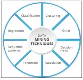
Regression Analysis (RA) is a group of factual devices that can help from numerous points of view to anticipate things of different segments. RA is utilized to construct numerical models to anticipate the estimation of one variable from learning of another. Figure 1 shows the eight different types of data mining techniques.

Most regularly, RA evaluates the contingent desire for the needy variable given the free factors – that is, the normal estimation of the needy variable when the autonomous factors are fixed. Less usually,

Revised Manuscript Received on June 05, 2019

Dr. K. K. Baseer, Associate Professor of IT & Member, Data Analytics Research Center, Sree Vidyanikethan Engg. College, Tirupati, India E-mail: [email protected]

Vikram Neerugatti, Research Scholar, Department of CSE, SVUCE, Sri Venkateswara University, Tirupati, India. E-mail:

[email protected]

Dr. Sandhya Tatekalva, Academic Consultant, Department of Computer Science, S.V. University, Tiruapti, India. E-mail:

[email protected]

Dr. Akella Amarendra Babu, Department of Computer Science and Engineering, St. Martin’s Engineering College, Telangana, India E-mail:

[email protected]

the attention is on a quantile, or other area parameter of the contingent circulation of the reliant variable given the autonomous factors. Figure 2 shows the machine learning types.

In all cases, a regression function is used to assess the independent variables. In RA, it is additionally important to describe the variety of the needy variable around the expectation of the regression function using probability distribution.

Figure 3 shows the three metrics used in regression. They are linear, logistic, exponential, nonlinear, polynomial, etc. commonly used regression is linear regression. In this we developed linear regression, multi variate linear regression, Gaussian regression using kernel, polynomial regression [1] [2] [3].

All these regression methods are done by using machine learning. We used Mat lab platform to solve regression analysis and developed various functions like gradient descent, cost compute, normalization. For experimental, vehicle data is used like velocity with which traffic move’s, gradient, actual velocity to predict the velocity profile of the vehicle. From these predicted range of a vehicle. By using different models of regression we come to conclusion which model predicts best and fits the data to the best.

K. K. Baseer, Vikram Neerugatti, Sandhya Tatekalva, Akella Amarendra Babu

S. No. Application Regression used to

1. Pharmaceutical company

 Assess the stability of the active ingredient in a drug.

 Predict its timeframe of realistic usability so as to meet FDA guidelines and

 Identify a reasonable lapse date for the medication.

2. Credit Card _company

 Predict month to month gift voucher deals.

 Improve yearly income projections .

3. Hotel Franchise  Identify a profile.  Predict potential customers.

4. Insurance company

[image:1.595.308.554.147.225.2]

 Determine the probability of a genuine issue existing.

Fig.1 Eight Data Mining Techniques (Courtesy: Google)

TABLE 1:APPLICATIONS OF REGRESSION

[image:1.595.73.244.426.590.2]

(2)

The paper is organized as follows: Section 2 presents prior art and challenges. Section 3 presents the analysis of regression and Section 4 gives the design and implementation of regression. Section 5 discusses the experimental results and Section 6 presents the conclusion of the paper.

II. PRIORART

A. Regression Analysis: Height vs Weight

Figure 4 shows the regression analysis on height vs weight.

B. Regression Analysis: Sleep vs Happiness

Figure 5 shows regression analysis on sleep vs happiness.

Simple linear regression is a model with a

single regressor x that has a relationship with a

response y that is a straight line.

Simple linear regression is a model with a single regressor x that has a relationship with a response y that is a straight line.

y = β0 + β1x + ε

where the intercept β0 and the slope β1 are unknown constants which is shown in figure 6.

On the off chance that there is more than one regressor, it is called multi variable regression. As a rule, the reaction variable y might be identified with k regressors, x1, x2,… ,xk, so that

y = β0 + β1x1 + β2x2 +…+ βkxk + ε

R-squared is a measure in insights of how close the information are to the fitted regression line. It is otherwise called the coefficient of assurance, or the coefficient of various conclusions for numerous regression [4].

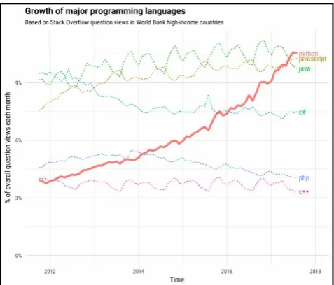
[image:2.595.49.277.69.251.2]

C. Regression Analysis: Growth of Programming Languages

Figure 7 shows the growth of programming languages with respect to number of questions views in each month.

III. SYSTEM ANALYSIS

The purpose of this work is to test various regression

IV. SYSTEMANALYSIS

The purpose of this work is to test various regression models on data to predict results. For this we had used matlab as a platform and worked on it. The test data was taken from vehicle data it contains map velocity which traffic moves, driver velocity and gradient. The outcome of this project is to come at a conclusion how regression was used in prediction. We tested for four models: linear, multivariate linear, polynomial and Gaussian regressions. For this we used machine learning algorithms to get the best without using the pre-defined functions in matlab [5] [6] [7] [8].

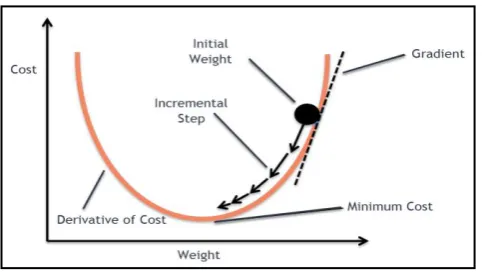
A. Gradient Descent

Gradient descent is an optimization algorithm used to minimize some function by iteratively moving in the direction of steepest descent as defined by the negative of the gradient shown in figure 8.

Fig.3 Metrics of Regression (Courtesy: Google)

Fig.4 RA with Height vs Weight (Courtesy: Google)

Fig.5 RA with Sleep vs Happiness (Courtesy: Google) Fig.6 Simple Regression Model (Courtesy: Google)

[image:2.595.309.548.308.512.2] [image:2.595.50.293.422.585.2] [image:2.595.39.293.656.774.2]

(3)

B Multi-variate linear regression(MVLR)

Multivariate Regression is one of the simplest Supervised Learning Algorithm used to estimates a single regression model with more than one outcome variable which is shown in figure 9.

 Use either SI (MKS) or CGS as primary units. (SI units are encouraged.) English units may be used as secondary units (in parentheses). An exception would be the use of English units as identifiers in trade, such 

 as “3.5-inch disk drive”.

The following are the steps need to follow to perform MVLR:

i. Selection of features ii. Normalization of feature

iii. Selection of Hypothesis and Cost function iv. Minimization of cost function

v. Test the hypothesis

B. Polynomial Regression(PA)

The relationship between the independent variable (x) and the dependent variable (y) is modeled as an nth degree polynomial in x is known to be PA which is shown in figure 10.

V. IMPLEMENTATION

Regression is implemented in matlab 2016a by using machine learning algorithms. The data we used was vehicle

data it contains vehicle velocity and gradient. We should predict actual velocity of a vehicle [9] [10].

A. Linear Regression

In this linear regression we had used gradient descent and cost compute functions without using pre-defined functions.

Where the hypothesis is given by the linear model:

Review that the parameters of your model are the _j values. These are the qualities you will acclimate to limit cost J. One approach to do this is to utilize the batch gradient descent calculation. In batch gradient descent, every cycle plays out the update.

With each step of gradient descent, your parameters come close to the optimal values that will achieve lowest cost J. B. Compute cost

function J =

computeCost(MapVelocity,ActualVelocity,theta) m=length(ActualVelocity);

J=0;

J=(sum((MapVelocity * theta –

ActualVelocity).^2))/(2*m); end

C. Multi variate linear regression

D. Polynomial regression data = xlsread('last.xlsx',1,'A2:B476');

t = data(:, 1); y = data(:, 2);

figure(1); hold on;

plot(t,y,'r^','MarkerFaceColor',[1,0,0],'MarkerSize ',8);

plot(t,y,'LineWidth',1.5); title('data');

xlabel('t'); ylabel('y'); grid on;

x1 = [ones(length(t),1),t];

a1 = solveMatrix(x1.'*x1,x1.'*y);

a1_1 = (x1.'*x1)\(x1.'*y);

[image:3.595.46.288.53.193.2]

f1 = @(t)a1(2)*t + a1(1); Fig.8 Gradient Descent (Courtesy: Google)

Fig.9 Multi-variate linear regression (Courtesy: Google)

[image:3.595.47.293.289.394.2]

(4)

figure(2); hold on; hold on; p1 = polyfit(t,y,1);

fp1 = @(t)p1(1)*t + p1(2);

plot(t,fp1(t),'LineWidth',1.5);

title('polyfit-1');xlabel('t');ylabel('y');grid on %% 2nd order

x2 = [ones(length(t),1),t,t.^2]; a2 = solveMatrix(x2.'*x2,x2.'*y); a2_1 = (x2.'*x2)\(x2.'*y);

f2 = @(t)a2(3)*t.^2 + a2(2)*t + a2(1); figure(4); hold on;

plot(t,f2(t),'LineWidth',1.5);

title('2');xlabel('t');ylabel('y');grid on; p2 = polyfit(t,y,2);

fp2 = @(t)p2(1)*t.^2 + p2(2)*t + p2(3); %% 3rd order

x3 = [ones(length(t),1),t,t.^2,t.^3]; a3 = solveMatrix(x3.'*x3,x3.'*y); a3_1 = (x3.'*x3)\(x3.'*y);

f3 = @(t)a3(4)*t.^3 + a3(3)*t.^2 + a3(2)*t + a3(1);

figure(6); hold on;

plot(t,y,'r^','MarkerFaceColor',[1,0,0],'MarkerSize',8 );

fp3 = @(t)p3(1)*t.^3 + p3(2)*t.^2 + p3(3)*t + p3(4);

%% 4th order

x4 = [ones(length(t),1),t,t.^2,t.^3,t.^4]; a4 = solveMatrix(x4.'*x4,x4.'*y); a4_1 = (x4.'*x4)\(x4.'*y);

f4 = @(t)a4(5)*t.^4 + a4(4)*t.^3 + a4(3)*t.^2 + a4(2)*t + a4(1);

figure(8); hold on;

fp4 = @(t)p4(1)*t.^4 + p4(2)*t.^3 + p4(3)*t.^2 +

p4(4)*t + p4(5);

E. Gaussian regression

In this model we used kernel parameters for getting results. We used noise parameter to remove outliers of the data.

We had used gram matrix to store the data from the results. Later we had used covariance matrix for the regression [11] [12].

At last we used kernel to predict the output.

VI. RESULTS

The results for that test data using various regression models. They are:

A. Linear regression:

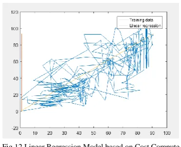
By performing linear regression, Theta found by gradient descent: -0.152761 1.032296.

(5)

[image:5.595.316.542.47.691.2]

Figure 11 and 12 shows the linear regression model based on gradient descent, cost compute.

B. Multi-variate Linear Regression

Figure 13 shows the multi-variate linear regression with number of iterations vs cost.

C. Polynomial Regression

[image:5.595.71.257.51.202.2]

Figure 14 (a), (b), and (c) shows the polynomial regression with polyfit-1 to polyfit-3.

Fig.12 Linear Regression Model based on Cost Compute

Fig.13 Multi-variate linear regression with gradient descent

Fig. 14(c) Polynomial Regression with polyfit-3

Fig. 14(b) Polynomial Regression with polyfit-2

[image:5.595.319.534.53.380.2]

Fig. 14(a) Polynomial Regression with polyfit-1

[image:5.595.54.261.246.386.2] [image:5.595.321.545.413.675.2] [image:5.595.53.261.585.751.2]

(6)

VII. CONCLUSIONANDFUTUREWORKS In this work, we had discussed various regression models and their uses. Regression analysis helps us to predict things accurate; we can develop this using exponential, logistic type of regression. In this we analyzed various models and predicted velocity of a vehicle. In this work we had examined relationship between variables. One advantage of a regression model over factor or cluster analysis is that the regression model can be used to obtain an estimate of the actual amount of change in a dependent variable that occurs as a result of a change in an independent variable. In this we used matlab software and wrote a code for that without using pre-defined functions like fitln(), fitlm(), etc. we also developed using 2 dependent variables to one independent variable. We also plotted the data to the best fit and analyzed it by changing the learning rate and iterations.

The future works of this work was to develop multiple regressions. When dealing with many variables, all of which are measured at no more than the nominal level, a multivariate model produces tables of 3, 4, 5 or more dimensions. These are very difficult to analyze, although some researchers use log linear models to examine these. The other difficulty of these models is that even where relationships among variables are found; it may be difficult to describe them in an understandable manner. We had developed only linear regression, but there is a need to develop non-linear regression.

REFERENCES

1. Sergios Theodoridis, Konstantinos Koutroumbas, Pattern Recognition, Academic Press, Second Edition, 2009.

2. Richard Duda, Peter E Hart, David G Stork, Pattern Classification, John Wiley and Sons, Second Edition, 2001.

3. Christopher M.Bishop, Pattern Recognition and Machine Learning, Springer Publications 2006.

4. Ian. H. Witten and Eibe Frank, Data Mining: Practical Machine Learning Tools and Techniques, Elsevier Publication, Second Edition, 2005.

5. Joseph Adler, R in a Nutshell, O'Reily Publishers, 2010.

6. Pang-Ning Tan, Vipin Kumar and Michael Steinbach, Introduction to Data Mining, Pearson Education, 2006.

7. Jiawei Han and Micheline Kamber, Data Mining: Concepts and Techniques, Morgan Kaufmann Publishers, Second Edition, 2006. 8. “Mathworks” https://in.mathworks.com/products/matlab.html, drafted

on May 2019.

9. Akella Amarendra Babu, K. K. Baseer, “Online Speaker Recognition in Robust Speech Coder using Phonemic Distance Measurements For Security in the Military Net-Centric Communications”, International Journal of Pure and Applied Mathematics, Volume 120, No. 6, 2018, pp. 3747-3762.

10. Kushanoor Akbar, K. K. Baseer, Kalaga Anil, “Improving the Efficiency of Automotive Service with Recovery Analytics”, IADS-Computing Communications and Data Engineering Series, SSRN Elsevier Network, Volume 1, Issue 1, Feb-2018, pp. 1-6,

https://ssrn.com/author=2985413

11. C. Shoba Bindu, E. Sudheer Kumar, K. Khaja Baseer “An Essence of Soft Computing Techniques on Software Development Life Cycle” at CSI Communications, Volume No.40, Issue No. 12, ISSN No. 0970-647X, pp. 13-17, March 2017.

12. K. K. Baseer, A. Rama Mohan Reddy, C. Shoba Bindu, “FPYM: Development and Application of a Fuzzy based Poka-Yoke Model for

the Improvement of Software Performance”, Inder Science-International Journal of Innovative Computing and Applications, Volume 8, No. 2, June, 2017, pp. 65-80, DOI: 10.1504/IJICA.2017.10005901

AUTHORSPROFILE

Dr. K. K. Baseer obtained his Bachelor of Technology and Master of Technology degrees in Computer Science and Engineering from JNTUH, Hyderabad and Ph.D. degree from JNTUA University, Ananthapuramu, India. At present working as an Associate Professor in department of Information Technology, Sree Vidyanikethan Engineering College, Tirupati, A.P., INDIA. His areas of interest include Data Science, Software Engineering, Software Architecture, Service Oriented Architecture, Internet of Plants (IoP) and other latest trends in technology. He has more than 11 years of experience in both teaching and industry in the area of Computer Science and Engineering. He is a member of IAENG, CSI, IEAE and IISCA.

Mr VikramNeerugatti, is Working on Internet of Things on IoT at Sri Venkateswara University, Tirupati.He Pursuing his PhD in the area of Internet of Things (IoT) and his research Contributes are to provide detection and prevention mechanisms for RPL attacks like Sinkhole, Black hole, Wormhole, Rank attack, etc in IoT. He completed his Bachelors (B.Tech) & Master’s (M.Tech) Degree in the Specialization of Computer Science and Engineering at JNTUA. He has M.S Degree from Brain wells University, London, UK. He has more than 10 years teaching experience from various Institutions like NIT, Goa, Sri Vidyanikhethan, A. Rangampeta,Sri Venkateswara University, Tirupati and Sri Venkateswara College of Engineering, Chittoor. He has more than 5 years of Research Experience form NIT Goa and S. V University, Tirupati. He has attended more than 50 Workshops specifically in the area of IoT. He has published 15+ National and International Conferences and Journals. He got 6 best research paper awards. Recently he got Dr. B.R. Ambedkar Research Fellowship award for his innovative research contributions. His research areas are Internet of Things, Fog Computing, Cloud Computing, etc. He acted as a Resource personfor morethan 20 workshops specifically in the domain of the IoT& Fog Computing in various institutions like Sri Venkateswara University, Sri PadmavathiMahilaViswavidyalam, Tirupati,Chdalavadavenkatasubbamma engineering college, tirupati,Sir Vidyanekithan Engineering College, etc.

Dr. Sandhya Tatekalva, Dept. Of Computer Science, S.V.University, Tirupati, A.P., has completed MCA and Ph.D. in computer Science, Rayalaseema University, Published 20+ journals and conferences. research experience are image mining, internet of things, data science. got best researched award.