Computed Tomography Medical Image Compression using Conjugate Gradient

(1)

International Journal of Innovative Technology and Exploring Engineering (IJITEE) ISSN: 2278-3075,Volume-8 Issue-12, October 2019



Abstract: Image compression which is a subset of data compression plays a crucial task in medical field. The medical images like CT, MRI, PET scan and X-Ray imagery which is a huge data, should be compressed to facilitate storage capacity without losing its details to diagnose the patient correctly. Now a days artificial neural network is being widely researched in the field of image processing. This paper examines the performance of a feed forward artificial neural network with learning algorithm as conjugate gradient. Various update parameters are considered in conjugate gradient methodology. This work performs a comparison between Conjugate gradient technique and Gradient Descent algorithm. MSE and PSNR are used as quality metrics. The investigation is carried on CT scan of lower abdomen medical image.

Keywords: Neural Network, Compression, Gradient Descent, Conjugate Gradient, Performance Metrics

I. INTRODUCTION

Because of the vast development in communication and multimedia technology, image storage is a key task in today‟s scenario. With the current major growth in e-health, telemedicine, teleconsultation and teleradiology, the interest of researching in the field of medical image compression is being increased [1]. In the medical field, storing a huge data in terms of Scan and X-Ray imaging is a challenge[2]. Therefore, compression is an important task in medical field. Medical images should be compressed in such a way that the subjective quality of the medical image is good so that the patient is diagnosed correctly i.e. the image is compressed while preserving its details. There are two methods of compressing an image , Lossless and lossy. Lossless compression technique recovers the original image accurately. Lossy compression technique removes psycho visual redundancies and attains higher compression ratios while degrading the image quality [3].The procedure of image compression can be illustrated in Fig. 1.

Revised Manuscript Received on October 05, 2019.

S.Saradha Rani, Dept.of ECE ,GITAM(deemed to be university),Visakhapatnam,Andhra Pradesh,India.

G.Sasibhushana Rao, Dept.of ECE, AU College of Engineering(A),AU,Visakhapatnam, Andhra Pradesh, India.

B.Prabhakara Rao, Dept.of ECE,JNT University, Kakinada, Andhra Pradesh,India.

Fig.1. Diagrammatic representation of an image compression process

In this paper, Section II explains the basic structure of a neural network, Section III deals with the training algorithm, Section IV gives the performance metrics and in Section V results are discussed.

II. BASICSTRUCTUREOFANEURALNETWORK

Recently, implementing artificial neural network in the applications of image processing has been increased. Implementing NN for compressing the image comes under lossy compression method. Hence performance metrics are used to remark on method appropriateness [4].

An artificial neural network comprises of three layers namely input layer, hidden layer and an output layer [5]. The basic structure of a neural network is shown in Fig. 2. The NN is trained using Conjugate Gradient algorithm to compress an image. The number of neurons in hidden layer is comparatively less than the number of neurons in the input layer. The choice of number of hidden nodes depends on the compression ratio required. The unprocessed image is applied to the input node. The hidden layer output in concert with the weights related to the output nodes forms the compressed image [6,7].At the output layer, the decompressed image is obtained by multiplying the weights with the output at the hidden layer [8,9,10].

Computed Tomography Medical Image

Compression using Conjugate Gradient

(2)

Fig.2.Basic structure of a Neural Network

III. CONJUGATEGRADIENT

In this paper gradient descent method is compared with conjugate gradient.

One of the well known and most popular iterative techniques is the conjugate gradient. The word conjugate stands for orthogonal, and hence orthogonal gradients[11,12]. The minimum of a function ,say Q(y), is obtained by setting the gradient equal to zero.

i.e., ∇𝑄 𝑦 = 𝐴𝑦 − 𝑏 = 0

(1) The solution is obtained by solving the residual

r



b



Ay

(2) The sequence {yk} is such that the residual is orthogonal

and is given by,

𝑦𝑘 +1= 𝑦𝑘+ 𝛼𝑘𝑝𝑘

(3)

Where pk is the search direction vector, αk is a scalar that

determines the step length.

The search direction is given by,

𝑝𝑘 +1= 𝑟𝑘+1+ 𝛽𝑘𝑝𝑘

(4)

The β which is the update parameter is of the various forms and is given as follows:

Fletcher-Reeves Update:

1 1 k

 



k T k

r r

 (5)

Polak- Ribiere Update:

𝛽𝑘= ∆𝑟_𝑘−1𝑇 𝑟_𝑘 𝑟_{𝑘 −1}𝑇 𝑟𝑘−1

(6)

Powell- Beale Restarts:

In conjugate gradient methods, the search direction resets from time to time to the negative gradient. Powell- Beale proposed a reset method that restarts if the orthogonality between the current and previous gradients is small. This is verified with following condition,

2

1 k

0 .

2

k

T

k

g





(7)

Conjugate gradient comprises of the following steps: (i) For the first iteration, start searching in the direction of the steepest descent i.e. gradient negative.

(ii) Compute the steepest direction [13]

(iii) Calculate the update parameter by using any one of the above formulas.

(iv) Update the conjugate direction and position using the above formulas.

(v) Repeat steps (ii) to (iv) until maximum iterations reached.

IV. METHODOLOGY

The conjugate gradient algorithm and feed forward neural network is considered. Feed forward network is used for coding the image. First, an image is divided into sub-blocks and is scanned into a vector. All original image blocks is transmitted through the hidden layer consisting of H neurons with S synapses each, and is measured by chosen weight matrix. If H<S, such scheme produces image compression. The outputs of the hidden layer is passed through the output layer to obtain the decompressed image. Hence the hidden layer output is the compressed image and the output at the output layer is the decompressed image.

The network is trained using conjugate gradient with different update parameter.

A. Algorithm

a) Read the original image

b) Divide the image into blocks and scan into a vector. c) Initialize the neurons

d) Apply the scanned vectors to each neuron in the input layer.

e) With the logic involved and the weights, accomplish the process and pass to the hidden layer.

f) Repeat the step in e)

(3)

Fig.3.Flow chart describing the image compression V. RESULTSANDDISCUSSION

The image quality is calculated using the metrics like Mean Square Error, MSE; Peak Signal to Noise ratio, PSNR and structural similarity index measure, SSIM. These define the reconstructed image quality at the output layer of ANN. The MSE should be possibly small i.e. the mean square error must be zero for ideal decompression.

𝑀𝑆𝐸 = 1

𝑘𝑙 [𝑂 𝑚, 𝑛 − 𝑅 𝑚, 𝑛 ]

2 𝑙−1

𝑛=0 𝑘−1

𝑚 =0 (8)

𝑃𝑆𝑁𝑅 = 20 𝑙𝑜𝑔 𝑀𝑎𝑥𝑖

𝑀𝑆𝐸 dB (9)

Where, O and R indicates the original and reconstructed images and Maxi represents the maximum of the pixel value.

Compression Ratio,

𝐶𝑅 =𝑢𝑛𝑐𝑜𝑚𝑝𝑟𝑒𝑠𝑠𝑒𝑑 𝑖𝑚𝑎𝑔𝑒 𝑠𝑖𝑧𝑒

𝐶𝑜𝑚𝑝𝑟𝑒𝑠𝑠𝑒𝑑 𝑖𝑚𝑎𝑔𝑒 𝑠𝑖𝑧𝑒

(10)

Table- I: Performance Comparison Of Gradient Descent And Conjugate Gradient

Training Function

For 8 Hidden Nodes

MSE PSNR SSIM

gd 5956.1 10.3812 0.0242

gdm 6.5859e+03 9.9446 0.0188

gda 721.4530 19.5487 0.2685

gdx 593.6624 20.3954 0.4308

cgb 65.5299 29.9664 0.8776

cgf 123.6758 27.208 0.7554

cgp 153.9872 26.256 0.7519

scg 88.7754 28.6479 0.836

oss 192.9324 25.2768 0.6884

rp 151.2115 26.335 0.7234

Table- II: Performance Comparison Of Gradient Descent And Conjugate Gradient Training

Function

For 16 Hidden Nodes

MSE PSNR SSIM

gd 7.49E+03 9.3885 0.0115

gdm 7.5393e+03 9.3575 0.0073

gda 887.7975 18.6477 0.2184

gdx 564.0124 20.6179 0.4145

cgb 30.3989 33.3022 0.9341

cgf 81.7935 29.0036 0.8351

cgp 48.3789 31.2842 0.8974

scg 59.1106 30.4141 0.8875

oss 124.9324 27.1641 0.7907

rp 130.7546 26.9662 0.7506 Yes

No Start

Original Input Image

Divide image into blocks

Compute output values of all neurons at every layer

Calculate Error

Update weights and biases Stop

Criteria

(4)

[image:4.595.305.535.48.339.2]

Table- III: Training time comparison of gradient descent and conjugate gradient

Training Function

Training time

8 Hidden nodes 16 hidden nodes

gd 3.5553 3.8442

gdm 5.0523 5.3681

gda 5.0136 5.3241

gdx 5.1552 5.5554

cgb 7.3392 7.9363

cgf 7.1734 7.9947

cgp 7.4185 7.9472

scg 3.6001 5.0807

oss 6.7914 7.43

rp 3.6001 3.7956

The performance of a neural network using conjugate gradient is carried on Computer Tomography medical image. The neural network is created with one hidden layer. The image is compressed with „8; and „16‟ neurons in hidden layer. While, there are 64 neurons in the input and output layer.

Experiment has been carried on CT image with different training algorithms to test the performance of a Feed forward neural network. The experiment is done for „1000‟ epochs.

Table I compares the performance of gradient descent and conjugate gradient algorithms for „8‟ hidden nodes in terms of MSE, PSNR and SSIM. Conjugate gradient with Powell-Beale restart performs better than gradient descent with values MSE as 65.5299, PSNR as 29.9664 and SSIM as 0.8776.

Table II compares the performance of gradient descent and conjugate gradient algorithms for „16‟ hidden nodes in terms of MSE,PSNR and SSIM. Conjugate gradient with Powell-Beale restart performs better than gradient descent with values MSE as 30.3989, PSNR as 33.3022 and SSIM as 0.9341.

[image:4.595.58.280.54.323.2]

From Table I and Table II we can say that as number of hidden nodes increasing the quality of the image is also increasing. The compression ratio obtained for table I is 8:1 and for Table II is 4:1.

Table III illustrates the time required to train the network for „8‟ and „16‟ hidden nodes with different training functions. To train the network with conjugate gradient method requires more time than the time required to train the network with gradient descent algorithm for both „8‟ and „16‟ hidden nodes.

(a) Original Image (b) gd (c) gdm

(d) gda (e)gdx (f) cgb

(g) cgf (h) cgp (i) scg Fig.4.Original and Reconstructed images a) – i) of CT scanned lower abdomen medical images with 8 hidden nodes, using gradient descent and conjugate gradient.

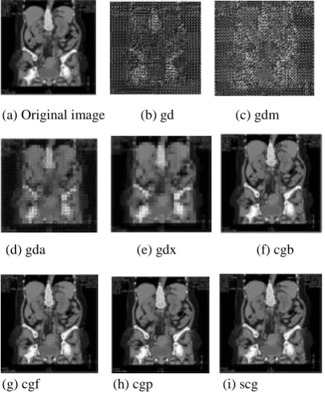
(a) Original image (b) gd (c) gdm

(d) gda (e) gdx (f) cgb

(g) cgf (h) cgp (i) scg

[image:4.595.311.543.398.680.2]

(5)

Fig.6. Graphs comparing MSE of various training functions for 8 and 16 hidden nodes

Fig.7. Graphs representing variation of PSNR with different training functions for 8 and 16 hidden nodes

Fig.8. Graphs representing variation of SSIM with different training functions for 8 and 16 hidden nodes.

Fig.9. Graphs representing variation of Training time with different training functions for 8 and 16 hidden

nodes.

Fig.4 and Fig.5 shows the original and reconstructed images of CT scanned lower abdomen medical image with 8 and 16 hidden neurons using gradient descent and conjugate gradient. From figures, it can be said that the subjective performance is good with conjugate gradient than gradient descent, that is, image is reconstructed with little distortion using CG than GD. Fig. 6 to Fig. 9 shows the variation of the quality measures like PSNR, MSE, SSIM and training time with various training algorithms for 8 and 16 hidden nodes.

VI. CONCLUSION

In this work, Conjugate gradient and gradient descent techniques that are based on artificial neural network is applied for compressing the CT scan of lower abdomen medical image. In conjugate gradient, the accurateness of the resultant outcome depends on the update parameter. The CG technique produces satisfactory results when compared to GD technique. The network is trained with 8x8 sub-blocks of image and tested for performance. A good image quality is obtained for CG, that is, it has high PSNR and SSIM, and low MSE. In image compression convergence time also play key task. The convergence of Conjugate gradient is earlier than gradient descent .The back propagation neural network with Conjugate gradient as learning algorithm improves the image compression and convergence time. Hence Conjugate gradient performs better both subjectively and objectively compared to gradient descent algorithm.

REFERENCES

1. N. Ayache, S. Duncan, , “Medical Image Analysis, Progress over two Decades and the Challenges Ahead”, IEEE Transactions on Pattern Analysis and Machine Intelligence, Vol. 22, No.1, pp. 85-106, 2000. 2. V Sowjanya, GS Rao, A Sarvani, "Investigation of Optimal Wavelet

Techniques for De-noising of MRI Brain Abnormal Image", International Conference on Computational Modeling and Security , Procedia Computer Science 85, 669-675, 2016.

0 1 2 3 4 5 6 7 8 9

gd gdm gda gdx cgb cgf cgp scg oss rp MSE

Training Functions

8 hidden nodes 16 hidden nodes

0 1 2 3 4 5 6 7 8 9

gd gdm gda gdx cgb cgf cgp scg oss rp PSNR

0 1 2 3 4 5 6 7 8 9

gd gdm gda gdx cgb cgf cgp scg oss rp SSIM

0 2 4 6 8 10

gd gdm gda gdx cgb cgf cgp scg oss rp Training

time

(6)

3. R. Gonzalez, E. Woods, “Digital Image Processing,” 3rd ed., Pearson Education, 2011.

4. PMK Prasad, M Kumar, GSB Rao," Design of Biortogonal Wavelets Based on Parameterized Filter for the Analysis of X-ray Images", Computational Intelligence in Data Mining-Volume 2, 99-110,2014.. 5. Rani M.L.P., Sasibhushana Rao G., Prabhakara Rao B.,”ANN

Application for Medical Image Denoising.”, In: Bansal J., Das K., Nagar A., Deep K., Ojha A. (eds) Soft Computing for Problem Solving. Advances in Intelligent Systems and Computing, vol 816. Springer, Singapore,2019..

6. K.S. Ng and L.M. Cheng, “Artificial Neural Network for Discrete Cosine Transform and Image Compression”, Proceedings of the fourth international conference on Document Analysis and Recognition, Vol. 2, pp. 675-678, 1997.

7. Emir Turajlic,”Application of Neural Networks to Compression of CT Images”, 978-1-5090-2902-0/16,IEEE,2016.

8. B.Perumal, M.Pallikonda Rajasekaran “A Hybrid Discrete Wavelet Transform with Neural Network Back Propagation Approach for Efficient medical Image Compression”,IEEE,2016.

9. JiaWei ,”Application of Hybrid BackPropagation Neural Network in Image Compression”, International Conference on Intelligent Computation Technology and Automation,IEEE, 2015.

10. Y. Shantikumar Singh, B. Pushpa Devi, Kh. Manglem Singh,” Image Compression using Multilayer Feed Forward Artificial Neural Networ with Conjugate Gradient”, 978-1-4673-4805-8/12,IEEE,2012. 11. Jyothi Kiran. G.C, “MRI Image Reconstruction: Using Non Linear

Conjugate Gradient Solution”, International Journal of Advances in Engineering & Technology, Jan. 2014.

12. Farhan Hussain , Jechang Jeong ,“Exploiting Deep Neural Networks for Digital Image Compression”,IEEE,2015

13. Saleh Ali Alsheri, “ Neural Network Technique for Image Compression”, IET image processing ,Vol. 10, issue 3,pp. 222-226, 2016.

AUTHORSPROFILE

S.Saradha Rani received B.Tech. in ECE from JNTU, Hyderabad, Andhra Pradesh in 2005 and M.Tech. in Radar & Microwave Engineering from Andhra University, Visakhapatnam, India in 2009 respectively. She is now working as Assistant Professor in GITAM(Deemed to be University), India. She is pursuing PhD degree in Image Processing at JNTUK, Kakinada. Her research interests include image and video processing and communications.

Prof.GottapuSasibhushana Rao is Professor in the Department of Electronics & Communication Engineering, Andhra University College of Engineering, Visakhapatnam, India. He is a senior member of IEEE, fellow of IETE, member of IEEE communication Society, Indian Geophysical Union (IGU) and International Global Navigation Satellite System (IGNSS), Australia. Prof. Rao was also the Indian member in the International Civil Aviation organization (ICAO), Canada working group for developing SARPS. He has published more than 485 Technical and research papers in different National / International conferences and Journals. His current research areas includes cellular and mobile communication, GPS, Bio medical and signal processing, under water image processing and optimization techniques.