An Improved Artificial Bees Colony Algorithm to Solve Minimal Exposure Problem in Wireless Sensor Networks

(1)

International Journal of Innovative Technology and Exploring Engineering (IJITEE) ISSN: 2278-3075, Volume-9 Issue-1, November 2019

An Improved Artificial Bees Colony Algorithm to

Solve Minimal Exposure Problem in Wireless

Sensor Networks

S.S.Aravinth, J.Senthilkumar, V.Mohanraj, Y.Suresh,

ABSTRACT: The problem of exposure, which is associated with the quality of coverage, is a basic issue faced in wireless sensor networks. Search for the Minimum Exposure Path (MEP) is one among the crucial problems in Wireless Sensor Networks (WSNs). The exposure with respect to the MEP is one of the indicators used for measuring the coverage quality of a WSN, depicting the efficiency with which the monitoring of a mobile target is done all along the sensing field. The available hybrid technique does not have sufficient accuracy to get the MEP, which is too complicated, and is not suitable to networks having heterogeneous sensor nodes, or in large number, or an all-sensor field intensity function. In order to get over these problems, an Improved Artificial Bee Colony (IABC) model is introduced for the MEP problem associated with getting the optimal shortest path in this research work. The IABC model exhibits an extensive use of energy and data congestion will happen. In order to have an efficient resolution to the data congestion problem, Prim’s algorithm has introduced the link level congestion scenario. Also for effective solving of this issue, in accordance with the features of the node, a semi Hidden Markov Model is developed to solve the problem of energy efficiency in WSN model. A number of experiments were carried out, and the results show that the proposed model and the designed IABC can help in increasing the solution accuracy and can be useful to not just the heterogeneous sensors’ case but also the scenario in where there are a big number of sensor nodes and also an all-sensor field intensity function.

Keywords: Minimal Exposure Problem (MEP), Wireless Sensor Network (WSN), Semi Hidden Markov Model, Prims Algorithm, and Improved Artificial Bee Colony (IABC).

I. INTRODUCTION

A popular technique for the evaluation of the coverage quality of Wireless Sensor Networks (WSNs) is uses exposure in the form of a measure, particularly in problems of barrier coverage. On analyzing all of the studies associated with exposure, discussions about the Minimal Exposure Path (MEP) problem has remained predominant in the research works carried out recently. The aim of the problem is to get a path along which an adversary can get through the sensing field with the least probability of being identified. This path and also its exposure value facilitate the designers of network infrastructure to find the worst-case coverage associated with the WSN and make required enhancements. Most of the earlier research work was focused on the MEP problem under the presumption that none of the environmental factors like vibration, temperature, etc., cause errors in real WSN systems.

Revised Manuscript Received on November 05, 2019.

Mr.S.S.Aravinth, AP/CSE, Dhirajlal Gandhi College of Technology, Salem

Dr.J.Senthilkumar, Prof/IT, Sona College of Technology, Salem

Dr.V.Mohanraj, Prof/IT, Sona College of Technology, Salem

Dr.Y.Suresh, Prof/IT, Sona College of Technology, Salem

Many applications of WSNs, including military applications, civilian applications etc., need that the network can identify the intrusions occurring in the region of interest. Hence, as a basic issue faced in wireless sensor networks, the coverage of intrusion-paths has a significant role to play in the applications employed for intrusions detection [1]. In [2] first, the problem is translated into an optimization problem with constraints. Due to the tediousness involved in getting a solution owing to the high nonlinearity and high dimensional complexity of the model, in addition to the specific characteristics of the issue, a hybrid genetic algorithm is introduced to get the solutions. This work also corroborates the same with a proof for the convergence of the newly developed algorithm.

A set of simulation experiments show that the newly developed optimization model with constraints and the hybrid genetic algorithm can help in efficiently solving the problem of proposed minimal exposure path. In [3] a new crossover operator is developed on the basis of the features of the sensor node coverage, and a novel local search approach is introduced, and an upside-down operator to elude from the local optima is designed. Combining all these, a Hybrid Genetic Algorithm (HGA) is introduced for the NFE model and its global convergence with probability one is shown to prove. In [4] first the MEP problem is formulated on the basis of the Probabilistic Coverage Model with noise (PM-MEP) and a new specification of the exposure metric for this model is introduced.

The PM-based-MEP is then translated into a numerically functional extreme that is higher dimensional, non-differential and non-linear. In order to resolve the MEP problem in wireless sensor networks with more efficiency, in [5] an algorithm known as Target Guiding Self-Avoiding Random Walk with Intersection (TGSARWI) is proposed, which imitates the behavior of a set of random walkers who try to find the path to their destinations in a queer region. Dijkstra algorithm (DA) is used for solving the MEP problem in a sub-network created by several connected paths generated by the walkers. Simulations reveal that the path exposure got by TGSARWI DA approximately equals to that obtained by DA in the global network (Global DA), while the computational time complexity is much lesser. In [6] introduced a new optimization problem model that is high–dimensional and highly non–linear, and an efficient hybrid particle swarm algorithm is developed for finding a solution to the proposed model to get the MEP. This can yield meaningful information on the coverage quality assessment of the wireless sensor network. Many approaches that solve MEP problem are not desirable or they can lead to failures in the heterogeneous scenario. Especially, exposure can be

informally indicated to be the

average capability of

(2)

Networks

sensors deployment field, and the MEP problem attempts to get a path between two certain points such that the overall exposure achieved from the sensors is reduced.

Song et al. [7] first introduced a PA that depends on the flow conductivity model to find a solution to the problem of minimal exposure in wireless sensor networks, which can be translated into the conventional Steiner tree problem in graphs. In [8] this algorithm was improved, and their algorithm revealed a performance that is quite identical to two classical algorithms, the 1.55 worst-case ratio algorithms and the tabu search algorithm. In [9] a biological model of physarum was used for designing a new biology-inspired optimization algorithm for MEP. At first, MEP and the associated models were formulated, and then MEP was converted into the Steiner problem through the discretization of the monitoring field to a large-scale weighted grid. Influenced by the path-discovering potential of physarum, a biological optimization solution is developed in order to get the minimal exposure road-network among multiple points of interest, and a Physarum Optimization Algorithm (POA) is presented. Also, POA can be utilized for resolving the common Steiner problem.

In [10] the minimal exposure path in a region, which includes heterogeneous sensor nodes and different hurdles, is analyzed. First, two exposure-based coverage models are created to define the detection patterns of both unidirectional and directional sensing units. Depending on the models, the exposure value of a random path can be mathematically obtained. Subsequently, the obstacle-avoidance minimal exposure path searching (OMEPS) algorithm is introduced to get the minimal exposure path in an environment, which has hurdles. Along with looking for regions have a poor extent of coverage, OMEPS navigates the mobile objects through the coverage holes resulting due to obstacles without bothering about exposure.

In [11] analyzed the MEP problem for two diverse kinds of directional sensing models, which include the binary sector model and directional sensitivity model. For the binary sector model, a special Voronoi diagram, known as sector centroids-based Voronoi diagram is constructed, to translate the minimal exposure path problem from a continuous geometric problem to a discrete geometric problem. A new artificial-potential scheme [12] is introduced for planning the MEP of several vehicles in a dynamic environment having several mobile sensors, and a number of fixed hurdles. This technique exhibits various benefits over the available schemes, like the capability of computing multiple MEPs online, when preventing mutual collusions, in addition to the collisions occurring with obstacles detection while moving.

In [13] presented the first thorough treatment done to the problem, developing an approximation algorithm for the MEP problem with assured performance features. In [14] introduced an exposure path algorithm for a point and path in sensor networks. The fuzzy information exposure path of a point is specified to be the function of the distance between the sensors and objects. Within a predefined distance, as the distance reduces, the exposure gets higher. In [15] introduced a bond-percolation theory based approach, which maps the problem of exposure path into a bond percolation model.

In [16] suggested a Genetic Algorithm (GA)-based solution, which targets at attaining lesser exposure, scalability, and rapid convergence. A new flat binary chromosome encoding

approach and the respective crossover and mutation operators are developed. Geometric knowledge is included to considerably boost the rate of convergence. In [17], to prevent the loose bounds of critical density, a bond percolation-based approach is introduced to map the exposure-path problem into a 3D uniform lattice.

In [18] is suggested a new MEP problem whose requirement is that the path has to be along some edge of a protected region. As the respective weight graph model is unable to be established, the actual classic technique (grid-based approach) used in resolving the actual MEP problem does not function as desired for the proposed MEP problem afterwards.

At first, it is converted into a continuous optimization problem, and then a Improved Artificial Bee Colony (IABC) algorithm is designed to resolve this complicated optimal problem. Hence, there is a need to get a WSN network having a reduced exposure, which is more complicated than getting a MEP. For solving this problem, in this research work, a Semi-Hidden Markov Model (SHMM) algorithm is introduced for solving the MEP in WSNs.

The important contribution made by the research work is as given: The MEP objective is obtained with the help of the IABC model and as for the congestion and data loss problem; it is resolved by designing the prims algorithm. Semi Hidden Markov Models (SHMMs) is helpful in resolving the MEP detection with energy efficiency. Each SHMM state indicates a set of general continuous target-sensor orientations in which signal data with comparative invariance. The experiments are carried out for the proposed technique and the existing approach on the basis of few useful parameters including Throughput, Delay and Exposure. The remaining segment of this research work is organized as given. Section 2 introduces the technical prelims and devises the problem of minimal exposure for WSNs and the IABC algorithm is proposed for avoiding the minimal exposure problem faced with SHMM. The results of simulation and the performance analysis are given in Section 3, and the conclusions are provided in Section 4.

II. PROPOSED METHODOLOGY

(3)

Fig.1.Proposed Methodology 1.1. Minimal Exposure Path (MEP) Problem

Exposure is defined to be a measure of the probability of a target being detected within the sensing field, and it is associated with the sensitivity of every sensor node. Getting the MEP facilitates the targeted implementation of more sensors that can help in improving the quality of coverage. MEP is defined as a path lying

between and in the sensing

field having a minimal exposure and it is expressed by y* (1)

The MEP problem is about finding a path in which the exposure attains a minimum, whereas the

minimum could be attained by the

variation technique of extremum. The problem of continuous MEP is translated into a discrete problem in this section. Assuming that the identified field is a rectangular area, the rectangle can be split into grids [5].

In this, the sensor-identified grid is a weighted

connected network graph , where

indicates the set of all nodes and E refers to the set of all edges. Let represent the weight of the edge between two nodes and , which indicates the exposure of identified by all the sensors present in the grid field. As this graph is an undirected network graph, . Consider the length of the edge be , the coordinate of node vi be denoted by , the weight could be computed as below[3][18]:

(2)

When the exposure of each edge in the grid is obtained, the IABC algorithm can be helpful in finding the minimum exposure path between the source point and

target point . Hence, this research will use random walk for replicating the path-discovery process of a walker in an unknown region. After the generation of an adequate number of connected paths between and , IABC algorithm is helpful in searching for the minimum exposure path in the sub-network created by these connected paths. As with the path selection problem, the prim’s algorithm is used for avoiding the congestion problem in WSN.

1.1.1. Prim’s algorithm for congestion loss

In this section a Steiner tree and grid structure is used for generating an initial topology and Prim’s algorithm for reducing the data loss rate. If there is congestion by which the data loss is increased, by choosing and replacing the nodes of the same level, the Prim’s algorithm [19] tries to minimize the data loss. The Prim’s algorithm is used at first to the proposed system to decide the Steiner tree and then the load flow analysis is carried out to know the amount of losses and a resource control algorithm was applied in the form of a factor for controlling the congestion faced in wireless sensor networks. In Prims algorithm, the information is sent by incorporating the two labels of a vertex, which include the closest tree vertex and the length of the corresponding edge. Vertices, which are not close to any of the tree vertices, can be given the ∞ label signifying their "infinite" distance to the tree vertices and a null label for the name of the nearest tree vertex. Making use of such labels, getting the next subsequent vertex to be added to the current tree T = (VT, ET) is found to be a simple task of obtaining a vertex having the least distance label in the set V – VT.

Algorithm 1. Prims algorithm

1. Correlate with every vertex v of the graph a number C[v] (cost of a connection to v(weight of the edges ) and an edge E[v] (the edge connection). For initializing these values, fix all the values of C[v] to +∞ (or to any number greater than the maximum edge weight) and fix every E[v] to a special flag value specifying that no edge connects v to previous vertices.

2. Initialize an empty forest F and a set Q of vertices, which have still not been added in F (at first, all of the vertices).

3. Repeat the below steps until Q becomes empty: 3.1. Find and eliminate a vertex v from Q with

the minimum probable value of C[v] 3.2. Include v to F and, if E[v] is not the

special flag value, then add E[v] also to F 3.3. Loop over the edges vw that connect v to

other vertices w. For every such edge, if w still is a part of Q and vw is of smaller weight compared to C[w], follow the steps below:

Fix C[w] to the cost of edge vw Fix E[w] to point to edge vw.

4. Return F

1.1.2. Path creation

In this stage, once the source node is selected, and the Steiner tree is generated. After the completion of the topology control stage, every node will have the capability of exchanging data with the maximum number of decided nodes with which it communicate in a single-hop. During this phase, any node being

chosen as the source node will assign the zero level to it and will send a Local Discovery WSN model

Form the graph structure

Congestion scenario in WSN (Link - level congestion) –Prims algorithm

Minimum Exposure Problem (MEP)-Improved Artificial Bee Colony (IABC) algorithm

Energy efficient -Semi Hidden Markov Model (SHMM)

(4)

Networks

(LD) message to the neighboring nodes that it had received in the topology control stage. Once this process terminates, the sink might get more than one LD packet from various nodes with diverse levels that occurs because of the various paths shown to reach the sink. Like it is stated before, WSNs comprises of nodes where each one of them have a particular transfer rate. In this kind of networks, if more than one node sends their data to a target node, then the cumulative transfer rate of data will go beyond its transmission rate. This will result in congestion. In such a condition, the target node will attempt stopping the receipt of data from more than one node. To achieve this, a pressure message will be transmitted to the nodes involved in transmitting data. So, one field in the ACK message will be set to false such that the target node’s reception of data is avoided in the next period. At last, the paths are chosen with the formula given below (3):

(3 )

Where signifies the occupied buffer, refers to the remaining energy occupied and represents the availability and non-availability of node. Using the above equation (3) on every neighboring node of WSN, the node having the highest value is selected.

1.1.3. Minimal Exposure Path (MEP) Problem -IABC In this section, MEP and the path-discovery by developing IABC optimization solution for multiple points of interest is first formulated. Artificial Bee Colony (ABC) algorithm helps in mimicking the behavior of the original bees searching for nectar. With the aim of overcoming the drawbacks of the standard ABC algorithm, an Improved ABC (IABC) algorithm is introduced in this section. Here, in this section, crossover operation is presented to extend the range of the MEP Problem search, and then the scanning approach is designed to remove the impact of worst local MEP Problem. In local optimization, the crossover operation helps in avoiding the local optimum problem with success and achieves more solutions in the local MEP Problem search space.

As per the earlier analysis, four selection processes are mentioned in the ABC algorithm; first one involves the global selection process, where the onlookers try to find a good food source for resolving local MEP; second one involves the local selection process, by which the leaders and onlookers look for the neighborhood path information; third one is a greedy selection process in which all the artificial bees find and perform a comparison between the old path and the new food sources to get a new path, then retrieve the best path; and fourth one is a stochastic selection process, which finds a correct path in the form of a food source. As with the MEP problem application, the bees build paths in various manners based on their roles. Leaders just repeat the earlier path of the iterative process without modifying the present WSN model. The scouts’ bee selects the next nectar source as below:

(4)

and signifies the bee colony and heuristic information for path , correspondingly, while α and β refers to the weight coefficient. Where indicates the probability that bee moves from node to in iteration .

(5)

Represents the nodes available for bee . Tabu k refers to the tabu list of bee k, which avoids the nodes that are already visited by bee k from getting visited again and again. And stands for the bee colony and heuristic information, correspondingly, while α and β refer to the weight coefficient.

In this section, a simple crossover operation improves the performance of ABC, whose step by step is as given: Step 1: Randomly choose the two paths from the solutions. Among the points in every path, randomly choose one crossover point.

Step 2: As the paths are chosen in random, the solution is possibly to be lower. Hence, the local optimization of the solution needs to be enhanced by a two-opt algorithm [20]. In two-opt algorithm, a crossover rate ( ) is introduced, which determined whether an optimal path selection in MEP problem requires a crossover. If is too big, it will reduce the algorithm’s convergence speed. In the primitive stages, the optimization has to be generally carried out over the highest possible MEP problem solution space. Adaptive algorithm with the intent of computation of the crossover rate is as below:

(6)

Where and represent the minimum and maximum crossover rates, correspondingly,

(H is the number of paths in the net)

(7)

(N is the number of distribution centers)

(8)

Where T and t represent the maximum and current iteration generations, respectively. If the two paths present in an optimization cross at one point, the local optimization can be performed with efficiency by removing that crossover point. Here, in this research work, the improvement of the crossover phenomenon is done with the help of a scanning technique [21]. The step followed in the scanning technique is given below:

Initialization

The proposed scanning mechanism takes the angle between the nodes and central node into consideration; hence, the positions of these points have to be a known value. To achieve this, the scanning technique creates a coordinate system having the origin set to the central depot coordinates, and then plots a line running from the origin to the sensor point in two-dimensional space.

Crossover operation based on the scanning strategy The nodes are ordered with the help of their angular values, and their path numbers are then recorded. Beginning from the node having the smallest

(5)

modified. But, the new path may have been scanned already, which involves a phenomenon known as fallback. In case the sensor points present in one path are contiguous and never face the fallback phenomenon, then that path doesn’t intersect any other path. The fallback phenomenon specifies a probable intersection. Then the possibly crossing path gets checked in the tabu list. In case the path resides is in the tabu list, then that algorithm decides if a crossover point exists between two paths. In case the result is negative, then the scanning goes on. When the scan attains the final node without facing the fallback phenomenon, then the algorithm terminates.

Two paths to judge whether they intersect

The intersection between two paths is judged as below: Suppose that there are two paths with end point of and and contains endpoint coordinates

of & .

1) If and

First, the slopes and of paths ab and cd are calculated as below:

(9)

If , then there can be no intersection between two paths; else, they may or may not cross. In the second scenario, the presence of the intersection is checked by computing the coordinates of the probable intersection. The expression for the abscissa of the potential intersection is:

, , (10)

where, and refer to two judgment parameters. If z is in between , , and , , then there is intersection; else, there is no intersection.

2) If or , then the two paths cannot cross. If and , the vertical axis of the potential intersection Z is calculated by adding into the linear equation of path . If is in between and , then there is intersection between two paths; else, they is no intersection. When the two paths intersect, the scanning schemes continue; else, the traversal goes on. In case there is no intersection after the traversal, the strategy continues that include these two paths are to the tabu list to prevent the judgments made again in next subsequent iterations.

Generation of new tours

The 2-opt algorithm is responsible for this. In case the two new paths can help in improving the solution, the old paths are replaced; else, the strategy terminates.

Final stage

Judgments are stopped if there is no practical crossover attained or when the algorithm has attained the particular iteration bound; else, the strategy continue. It is necessary to mention that the IABC can also help in resolving the MEP problem having heterogeneous sensor nodes and All-sensor Field Intensity Function.

1.1.4. Energy Efficient by Semi Hidden Markov Model Semi Hidden Markov Model (SHMM) is an expanded model of carrying out HMM employing a semi-Markov

chain with a differential staying duration for every state. The basic difference between HMM and SHMM exists in the number of observations for each state. Assuming that the WSN state has been categorized into hidden

states and the energy usage varies with

time. The entire specification of an SHMM has the following elements, specified as . The state transition probability distribution matrix is .

(11)

refers to the number of node states and indicates the state at time in SHMM. The conditional probability distribution matrix of

observing when given state is

parameter signifying the state duration

distribution , can be expressed as

(1 2)

where state stays for time units and the initial state probability distribution is expressed as

(13)

HSMM all require various state data to obtain diverse training HMMs or HSMMs and input test data to compute the respective emission probabilities that is actually the overall energy consumption in WSN models.

Kullback-Leibler Divergence (KLD) also called as Relative Entropy since the variance between two probability distributions . With the observation probability of the sensor state and the test state achieved, the KLD indicates the extent of deviation extent from the standard node state and can be computed by

(14)

A smaller range of the representsusage of a higher energy level. At last, a forward variable specified as the joint distribution of observation

sequence is defined and node state at

time when the model given for finding the energy rate is expressed as

(6)

Networks

where the energy emission observation of

state is , is and

indicate the state lasts from to , and refers to the maximal duration time.

III. EXPERIMENTAL RESULSTS AND DISCUSSION The Network Simulator known as NS-2 implementation platform has been introduced for establishing the newly introduced SHMM-IABC algorithm based MEP detection; 50 sensors have been spread on the 500x500m monitoring field having the sensing intensity. The operation of POA and H-GPSO with HMM algorithm were analyzed and then compared with the proposed approach, with the aim of evaluating the effectiveness and efficiency. The comparisons have been performed in terms of precision, convergence, and exposure values. Table 1 gives the simulation setup.

Table.1 Simulation setup

Simulation Parameters Values

Channel Wireless Channel

Mac 802.11

Antenna Type Omni antenna

Initial Energy 100 joules

Traffic type CBR

Agent UDP

Simulation area 500X500 meters

Number of sensor nodes 50

1.2. Precision

50 60 70 80 90 100

10 20 30 40 50

Pr

ec

isi

o

n

(%

)

Number of nodes

Dijkstra POA

H-GPSO with HMM IABC-SHMM

Fig.2. Precision Comparison vs. Number of Nodes Fig.2 illustrates the precision comparison results of the MEP detection techniques. With the precision along the x-axis and the number of sensor nodes in the y-axis, the precision is reduced as the number of sensor nodes is reduced. It is noticed from fig.2, that if there is an increase in the number of nodes in the network, then there is a rapid increase in the average Delay. It can be seen that the proposed IABC-SHMM technique exhibits higher precision results of 94%, while other Dijkstra , POA ,and H-GPSO with HMM

renders better precision results of 80%, 86%, and 92% at for 10 nodes . It is also noticed that the precision of IABC-SHMM is 14%,8% and 2% more than Dijkstra, POA and H-GPSO with HMM approach correspondingly.

1.3. Throughput

Fig.3.Throughput vs. No of Nodes

Fig.3 illustrates the results of comparison analysis of throughput obtained from the proposed IABC-SHMM, and the available POA and H-GPSO with HMM technique. It is observed that the proposed IABC-SHMM achieves a much better throughput in comparison with every other existing techniques includingDijkstra , POA and H-GPSO with HMM. The proposed IABC-SHMMscheme yields much better throughput results of 93.00%, while other techniques including Dijkstra, POA and H-GPSO with HMMyields comparatively lesser results of 71%, 77% and 86% for 50 nodes. The reason being, the proposed work is capable of finding the neighbor node with the help Prim’s that results in a better throughput with lesser rate of coverage.

1.4. Convergence

400 500 600 700 800 900 1000

10 20 30 40 50

N

u

m

b

e

r

o

f

it

e

r

a

ti

o

n

s

Number of nodes

Dijkstra POA

(7)

1.5. Energy Consumption

100 150 200 250 300 350

10 20 30 40 50

E

n

er

g

y

C

o

n

su

m

p

ti

o

n

(m

J

)

Number of nodes

Dijkstra POA

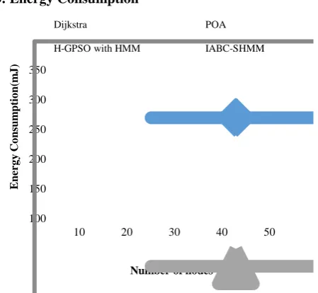
[image:7.595.323.530.52.260.2]

Fig.5. Energy consumption Vs No. of Nodes Fig.5 shows the association between the energy consumed in every technique and the number of nodes. As seen from the figure 5, the novelIABC-SHMM algorithm takes much lesser energy of 215 mJ, while other techniques including Dijkstra, POA and H-GPSO with HMM consumes a higher energy value of 305 mJ, 285 mJ and 235 mJ for 50 number of nodes correspondingly.As observed from the figure 5, the energy value will be decreased considerably after the initiation of MEP in sensor nodes present in WSN.

1.6. Exposure

8 8.5 9 9.5 10 10.5 11 11.5 12

10 20 30 40 50

E

x

p

o

su

re

Number of nodes

Dijkstra POA

Fig.6. Exposure Comparison vs. number of nodes Fig 6 illustrates the exposure values of different techniques and the number of nodes. The novel IABC-SHMM technique yields a much better exposure compared to other techniques, as the optimal path is identified with the help of IABC algorithm, and the target detection is performed with the help of SHMM incorporated with Prim’s. It can be observed that the proposed IABC-SHMM scheme achieves much better exposure results of 10.28, while other Dijkstra, POA and H-GPSO with HMM algorithm renders lesser exposure results of 9.2,9.45 and 10.1 for 50 no. of nodes respectively.

1.7. Delay

0.4 0.5 0.6 0.7 0.8 0.9 1

10 20 30 40 50

De

la

y

(m

il

li

s

e

c

o

n

d

s)

Number of Nodes

Dijkstra POA

Fig.7. Delay Vs No. of Nodes

Fig.7 illustrates the delay results of IABC-SHMM combined, and the existing techniques with the number of nodes given. It is noticed that the delay of proposed IABC-SHMM algorithm is much lesser compared to other techniques that gives lesser delay of 0.71 ms, while other approaches including Dijkstra, POA and HGPSO with HMM yields much better delay results of 0.86 ms, 0.81 ms and 0.74 ms for 50 nodes respectively.

IV. CONCLUSION AND FUTURE WORK This research work uses a novel technique of path-discovery and networking from this organism employing IABC with SHMM. In this IABC optimization, every junction node is navigated with the help of ordinary rules of interaction. If there was just one junction node, it would try to reach a local suboptimal solution employing SHMM. When the junction nodes communicate, they will converge over an approximate optimization employing Prim’s, instead of falling in local optima. Afterwards, the proposed IABC Optimization is used for solving the minimal exposure problem that could attain a sensor network having the approximate minimal exposure value. This article also yields a proof for the convergence of the novel algorithm. Elaborate experimental simulations help in evaluating the performance of IABC-SHMM for MEP, which attains the global approximate optimization by iterative evolution of individuals. The result shows that the novel optimization model with SHMM and the IABC algorithm can help in efficiently solving the mentioned minimal exposure path problem. Even though the approximate optimization could be attained under permissible computational complexity, more improvement could be achieved in the technique with a novel optimization algorithm enabled with coverage constraints as a the futuristic approach.

REFERENCES

1. Wang, B. Coverage Problems in Sensor Networks: a Survey. ACM Computing Surveys October 2011; 43(4), pp.1-53.

2. Feng, H., Luo, L., Wang, Y., Ye, M. and Dong, R., 2016. A novel minimal exposure path problem in wireless sensor networks and its solution algorithm. International Journal of Distributed Sensor

Networks, 12(8),

[image:7.595.58.283.69.276.2] [image:7.595.65.281.426.617.2]

(8)

Networks

3. Ye, M., Wang, Y., Dai, C. and Wang, X., 2015. A hybrid genetic algorithm for the minimum exposure path problem of wireless sensor networks based on a numerical functional extreme model. IEEE Transactions on Vehicular Technology, 65(10), pp.8644-8657. 4. Binh, H.T.T., Binh, N.T.M., Ngoc, N.H., Ly, D.T.H. and Nghia, N.D.,

2019. Efficient approximation approaches to minimal exposure path problem in probabilistic coverage model for wireless sensor networks. Applied Soft Computing, 76, pp.726-743.

5. Yang, T., Jiang, D., Fang, H., Tan, M., Xie, L. and Zhao, J., 2018. Target guiding self-avoiding random walk with intersection algorithm for minimum exposure path problem in wireless sensor networks. EURASIP Journal on Wireless Communications and Networking, 2018(1), pp.1-14.

6. Miao, Y., Wang, Y. and Jing–Xuan, W., 2015. Hybrid particle swarm algorithm for minimum exposure path problem in heterogeneous wireless sensor network. International Journal of Wireless and Mobile Computing, 8(1), pp.74-81.

7. Song, Y., Liu, L. and Ma, H., 2012, “A physarum-inspired algorithm for minimal exposure problem in wireless sensor networks”, In IEEE Wireless Communications and Networking Conference (WCNC) ,pp. 2151-2156.

8. Liu, L., Song, Y., Ma, H. and Zhang, X., 2012, Physarum optimization: A biology-inspired algorithm for minimal exposure path problem in wireless sensor networks. In 2012 Proceedings IEEE INFOCOM , pp. 1296-1304.

9. Song, Y., Liu, L., Ma, H. and Vasilakos, A.V., 2014. A biology-based algorithm to minimal exposure problem of wireless sensor networks. IEEE Transactions on Network and Service Management, 11(3), pp.417-430.

10. Liu, L., Han, G., Wang, H. and Wan, J., 2017. Obstacle-avoidance minimal exposure path for heterogeneous wireless sensor networks. Ad Hoc Networks, 55, pp.50-61.

11. Liu, L., Zhang, X. and Ma, H., 2014. Minimal exposure path algorithms for directional sensor networks. Wireless Communications and Mobile Computing, 14(10), pp.979-994.

12. Ferrari, S. and Foderaro, G., 2010, A potential field approach to finding minimum-exposure paths in wireless sensor networks. In 2010 IEEE International Conference on Robotics and Automation, pp. 335-341.

13. Djidjev, H.N., 2010. Approximation algorithms for computing minimum exposure paths in a sensor field. ACM Transactions on Sensor Networks (TOSN), 7(3), pp.23.

14. Wang, R., Gao, Y., Wan, W. and Mao, S., 2010, Fuzzy information exposure paths analysis in wireless sensor networks. In International Conference on Audio, Language and Image Processing , pp. 1619-1623.

15. Liu, L., Zhang, X. and Ma, H., 2013. Percolation theory-based exposure-path prevention for wireless sensor networks coverage in internet of things. IEEE Sensors Journal, 13(10), pp.3625-3636. 16. Xia, Na, Khuong Vu, and Rong Zheng. "Sensor placement for

minimum exposure in distributed active sensing networks." In 2010 IEEE Global Telecommunications Conference GLOBECOM 2010, pp. 1-6, 2010.

17. Liu, X., Kang, G. and Zhang, N., 2015. Percolation Theory-Based Exposure-Path Prevention for 3D-Wireless Sensor Networks Coverage. KSII Transactions on Internet & Information Systems, 9(1), pp.126-148.

18. Ye, M., Zhao, M. and Cheng, X., 2015, A New Minimum Exposure Path Problem and Its Solving Algorithm. In 2015 11th International Conference on Computational Intelligence and Security (CIS) , pp. 420-423.

19. Sudhakar T D, & Sakthivel, B & Hussain, N.S.N.. (2014). Loss minimization in distribution network using prim’s algorithm. International Journal of Applied Engineering Research. 9. 24033-24046.

20. Yu, B., Zhu, H., Cai, W., Ma, N., Kuang, Q. and Yao, B., 2013. Two-phase optimization approach to transit hub location–the case of Dalian. Journal of Transport Geography, 33, pp.62-71.