A Simulated shape recognition system using feature extraction

Rochester Institute of Technology

RIT Scholar Works

Theses

Thesis/Dissertation Collections

1989

A Simulated shape recognition system using feature

extraction

Wendy Pan

Follow this and additional works at:

http://scholarworks.rit.edu/theses

This Thesis is brought to you for free and open access by the Thesis/Dissertation Collections at RIT Scholar Works. It has been accepted for inclusion

Recommended Citation

Rochester Institute of Technology

School of Computer Science and Technology

A Simulated Shape Recognition System

Using Feature Extraction

by

Wendy Pan

A thesis, submitted to

The Faculty of the School of Computer Science and Technology

in partial fulfillment of the requirements for the degree of

Master of Science in Computer Sciences

Approved by:

John A. Biles

Edward R.

Salem

Peter G. Anderson

Permission to Reproduce

Title of Thesis:

A Simulated Shape Recognition System

Using Feature Extraction

I,

Wendy Pan,

prefer to be contacted each time a request for

reproduction is made.

I can be reached at the following

address:

19 Locke Drive

Pittsford,

NY 14534

ACKNOWLEDGEMENTS

I would _especially like to thank Prof. John Biles for

his encouragement, guidance, inspiration, and many helpful

comments. He also helped me greatly on improving my thesis

writing, I am _sincerely grateful. I would also like to thank

Prof. Edward Salem who reviewed the manuscript and kept me

ABSTRACT

A simulated shape recognition system _using feature

extraction was built as an aid for

designing

robot vision

systems. The simulation allows the user to study the effects

of image resolution and feature selection on the performance

of a vision system that tries to

identify

unknown 2-D

objects. Performance issues that can be studied include

identification accuracy and recognition speed as functions

of resolution and the size and makeup of the feature set. Two approaches to feature selection were studied as was a

nearest neighbor classification algorithm based on Mahalanobis distances.

Using

a pool of ten objects and

twelve features, the system was tested

by

performing studies of hypothetical visual recognition tasks.

Key

Words: robot vision, feature extraction, simulation,

TABLE OF CONTENTS

1. INTRODUCTION 1

2. BACKGROUND 5

2.1. Overview 6

2.2. Data Acquisition 6

2.2. 1. Visual Input Devices 6

2.2.2. Other Hardware 7

2.3. Data

Processing

7

2.3. 1. Segmentation 7

2.3.2. Edge Extraction 8

2.4. Classification 9

2.4. 1. Template Matching 9

2.4.2. Feature Extraction 10

2.4.3. Selection of a Feature Subset 15

2.4.4. Nearest Neighbor Classification Algorithm 16

2.5. Simulation

by

Shape Generation 19

IMPLEMENTATION 23

3.1. System Overview 23

3.2. Simulated Digitization 25

3.2. 1. Shape Generation 25

3.2.2. Effect of Grid Size 26

3.2.3.

Translation,

Rotation and

Scaling

29

3.2.4. Controlled Distortion 29

3.3. Classification

by

Feature Extraction 30

3.3.1. Feature Pool 31

3.3.2. Feature Selection 35

3.3.3. Classification 43

3.4. Flow Charts of Implementation 44

3.4. 1. System Data Flow Diagram 44

3.4.2. Hierarchical Process Diagram 44

3.4.3. Create and Store Objects 47 3.4.4. Select Reference Objects 47

3.4.5. Select a Feature Subset 47

3.4.6.

Identify

Unknown Objects 50

3.5. System Hardware and Software 52

4. RESULTS AND DISCUSSION 54

4.1. Graphic Representation of Edge-Extracted Objects 55

4. 1. 1. Objects in the Object Pool 55

4.1.2. Digitized Images without Distortion .... 61

4.1.3. Types of Distortion 61

4.1.4. Digitized Images with Distortion 62

4.2. Properties of the Objects in the Object Pool ... 63

4.2.1. Average Feature Values and Their Standard

Deviations 63

4.2.2. Mahalanobis Distances between Object

Classes with All Features 66

4.3. Selection of Reference Objects from the Object

Pool 68

4. 4. Effect of Resolution 69

4.5. Selection of a Feature Subset 75

4.5. 1. Elimination of Redundant Features 75

4.5.2. Selection of Features

by

Discrmination

Ability

79

4.5.3. Mahalanobis Distances between Object

4. 6. Classification of Unknown Objects 84

4.6.1. Generation of an Unknown Object

at a

Randomly

Distorted State 84

4.6.2. Confidence Level on Identification 85

5. CONCLUSION, FUTURE WORK AND OTHER APPLICATIONS 93

5.1. Future Work 93

5.2. Other Applications 95

BIBLIOGRAPHY 96

CHAPTER 1

INTRODUCTION

The patterns we encounter fall into two categories:

abstract and concrete. Examples of abstract items include

ideas and _arguments, and the recognition of such patterns is

beyond the scope of this study. Examples of concrete items

include characters, symbols, pictures, biomedical

images,

three-dimensional physical _objects, speech waveforms and

electrocardiograms CB0W84]. In the last couple of

decades,

extensive interest has focused on two types of concrete

pattern recognition problems: optical character recognition

and robot vision [BERT86]. This thesis focuses on the robot

vision area.

Many

robot vision (digital image processing) systems

also have been developed. Overviews of these systems are

presented in numerous papers CSUET863 [ZIMM833 CVANG86]. Robot

vision systems consist of a computer, an image memory bank

that is different from the computer RAM and connected to the

computer

bus,

an interface that connects the camera with the

image memory

bank,

and a sensor controller, which provides

the camera with the necessary synchronization signals.

In recent years, the power of digital image processing

also has been brought to the IBM PC and compatible

computers.

Imaging

Technology's PCVISION Frame Grabber

Frame Grabber that enables the user to perform low level

digital image _processing functions.

Among

them are image

averaging, image subtraction, convolution and edge _enhancing algorithms.

For a robot vision system to be capable of complex

automated assembly and inspection operations, it must be

able to perform in real time. The system's aim is to sort

randomly oriented objects on production lines at speeds of

about 10 objects/sec. As a result, some of the

functions,

such as edge detection and feature calculations, are

performed

by

dedicated hardware [CAGN863.

Although robot vision systems are

being

applied

increasingly

to manufacturing tasks, the installation of a

complete vision system is still expensive. Companies are

often reluctant to make such a major investment unless _they

are sure that the system can do the job.

This thesis describes a simulated shape recognition

system that can be used to do

feasibility

studies of the

suitability of robot vision systems. There is no need to go

through all the steps in

building

a vision system just for a

feasibility study because a simulated system can provide

useful data for

determining

whether to invest in an actual

vision system.

For instance, if one wants to differentiate a

bolt,

a

the

following

steps can be simulated

by directly feeding

the

digitized and edge extracted objects into a computer.

Using

a real robot vision system, one often needs to

image objects at random orientations and locations for a

teaching set. This can become tedious and time consuming,

but on a simulated _system, the

"picture"

in computer memory

can be easily rotated, translated and scaled in a matter of

seconds.

By doing

simulation, the

following

questions can be

answered before one seriously considers the installation of

a real vision system:

(a) What is the minimum required camera resolution,

64x64,

128x128 or . . . ? It is easy to digitize an object

mathematically at various grid sizes. The results will provide data to

help

in selecting the right kind of

electronic camera.

(b) What is the minimum number of features that need to

be examined to recognize a set of objects and what are those

features?

(c) What features take a

long

time to calculate? Can

these features be implemented in hardware?

Our objective was to provide a simple but complete

simulated shape recognition system to

help

decide on

appropriate resolution requirements and useful feature sets

for a robot vision system in a given domain. We have tested

This system has a simulated shape

digitizer,

procedures

to select and calculate feature values, and algorithms to

perform classification. Reference objects will undergo

controlled distortions to provide a range of feature values.

The average value and its standard deviation for each

feature of each type of object are then stored for future

comparison.

Chapter 2 of this thesis gives an overview of the

concepts and various components of a robot vision system.

Prior work also is reviewed.

Chapter 3 discusses the ways we have implemented our

simulated system. Some of our own ideas are presented here

and several flow charts are included to show the details of

our system.

Chapter 4 discusses the results of our work. Digitized

images with and without distortions are plotted. Feature

values and their standard deviations for various objects are tabulated. Mahalanobis distances between object pairs are

shown. The algorithms for selecting an effective feature

subset are also presented.

Finally,

identification and

confidence levels are examined on several unknown objects.

Chapter 5 concludes our work and also suggests how to

CHAPTER 2

BACKGROUND

2.1. Overview

In robot vision, one can divide an entire task into

three phases: data acquisition, data processing and decision

classification, as shown in Figure 2.1 [B0W84]. In the data

acquisition phase, light

intensity

is measured _by a sensor

and converted to a digital format suitable for computer

processing. The measured data then are used as the input to the data processing phase and are grouped into a set of

characteristic features as output. The classification phase

is implemented in the form of a set of decision functions.

In the

following

sections, we will discuss each phase in

great detail.

PHASE 1 > PHASE 2 > PHASE 3

DATA ACQUISITION

sensor detection digitization

DATA PROCESSING

segmentation

edge extraction

CLASSIFICATION

nearest neighbor

feature-extraction

2.2. Data Acquisition

An automatic visual inspection or robot vision system

consists of the

following

subsystems: _the part

handling

system, the optics and the sensor, the

illumination,

and the

computer system. Each of them is

briefly

described below.

2.2.1. Visual Input Devices

A variety of devices have been used for visual input to

robot vision systems. The most popular ones are solid-state

array cameras, linear arrays and laser scanners

CRAPA883 CMUND833 [AGIN803 .

Solid-state array cameras include CCD (charge-coupled

device) and CID (charge-injection device) cameras which

contain area arrays of photosensitive elements.

Uniformity

of response between elements of the array was a problem in

earlier devices, but high quality cameras available today have much improved uniformity.

Linear arrays are used where the scene to be scanned is

in continuous linear motion, as for example on a constantly

moving conveyor. The camera scans a line across the

conveyor, and the motion of the part produces the orthogonal direction of the scan. Cost reduction can be achieved

by

using a linear array instead of an area array.

Laser scanners generally use an arrangement of rotating

transmitted light from various angles. These systems are

capable of _extremely fast operation, but there are quite

expensive.

2.2.2. Other Hardware

In addition to visual input

devices,

there is other

required hardware

[SUET863,

depending

on the task. For

instance,

when

dealing

with parts

inspection,

there should

be a part

handling

_system, which consists of a

feeding

system for the transportation of the parts to the sensor and

a separation system for sorting the inspected objects. Proper illumination is also important. The goal is to

provide high contrast images to allow the objects of interest to be isolated from the background

by

simple

thresholding.

Also,

a computer is needed for data acquisition and

further processing.

2.3. Data Processing

When data acqusition is completed, some _processing of

data is needed. First of all, the object of interest should

be isolated. This step is called segmentation.

Secondly,

the

edges of the object are detected to simplify data

processing. This step is called edge extraction.

2.3.1. Segmentation

methods exist for _segmenting an image CSUET863. The easiest

way is called global

thresholding,

in which the objects are

separated _{from the background}

by

means of a fixed gray level

or threshold value. This thesis is restricted to examine

only

binary

images. If the gray level exceeds a threshold value, then that pixel is "on", otherwise it is "off".

If a frame contains more than one objects, connectivity

analysis [ROSE663 CAGIN803 is needed to break an image into

its connected components. For

instance,

if a wrench and a

nut are in an

image,

this analysis will indicate that there

are two separate objects so that each can be analyzed. This

analysis also detects any holes in an object. For this thesis, segmentation was not _necessary because the images that were processed were already segmented.

2.3.2. Edge Detection

Edge extraction CSHI0863CBOIE873 CCAEL873 CPAVI753 is

probably the most important step in image pattern

recognition. The purpose is to reduce the amount of data

points for the classification phase.

Edges are regions in which abrupt changes of brightness

occur. The edges in an image, then, can be extracted

by

detecting these changes. A gradient operator

[CHEN863,

which

the edge extraction is

by-passed,

since our mathematically

generated shapes constitute _only the edges.

2.4. Classification

Two major pattern recognition _approaches, template

matching and feature extraction, are discussed in this

section, although only the latter was implemented in our

system. Also two techniques for selecting a proper feature

subset, and algorithms for

doing

nearest neighbor pattern

classification CAGIN803 CCASH863 CGLEN873 are discussed.

2.4.1. Template

Matching

Direct image-matching,

frequently

called "mask matching"

or "template

matching" [AGIN803, is a

pixel-by-pixel comparison of one image (usually a

"live"

image) with

another (a stored image to be used as a reference or model). A fundamental limitation of template-matching systems

is that the two images to be compared must be in perfect

alignment for the comparison to be meaningful. If the

position of the object to be inspected is not precisely

known beforehand, some adjustments must be made. A brute-force technique to accomplish this is to compare images many

times, shifting one image with respect to the other between

comparisons, to find the amount of shift that maximizes the

correlation (minimizes the difference) between the images. This technique is widely used in recognizing printed

recognition (OCR) machines CTECH863 often require that "skew"

is within 2

degrees,

where skew is the angular

deviation from the proper orientation of a character.

Faster methods for template matching exist [HUTT873.

One method is to search _only a single row or column of the

image before shifting and scaling, selecting the translation

that yields the smallest difference in the single row or

column, and then calculating the difference between the two

entire images.

If one image is rotated with respect to the other, it

is possible to perform a rotation in software before

matching.

However,

rotation is much more time consuming than

shifting.

To increase speed, one also can match an image with

multiple templates [LI863, provided that each template has its own processor and the matching can be done in parallel.

2.4.2. Feature Extraction

Along

with template matching, there is another major

pattern recognition approach, called feature extraction

[BOW843CSHET863. The objective of feature extraction is to

reduce the dimensionality of the measurement space (pixels in a raw image) to a feature space suitable for the

application of pattern classification algorithms.

During

the

classification can be implemented on a _vastly reduced feature space.

In an N-feature space, an object is represented as an

N-dimensional vector, the vector components

being

the

different feature values. Examples of features commonly used

in current commercial vision systems are area, perimeter,

centroid (the center of _gravity), length of the minimum and

maximum radius _(Rmin, Rmax) from the centroid to the

perimeter, the angles of the minimum and maximum radius,

first and second invariant moments, and the length and width

of the

bounding box,

which is the smallest rectangle that

completely encloses the object.

Two dimensional moments have been used with success for

a number of image processing tasks. In the robotics

field,

moments are used for motion _tracking and for object

orientation calculations

[GOSH833,

scene matching [WONG783

and character recognition [CASH873 CHU623.

For a 2-D pattern, the moment of order (p+q) is defined

as

M =

ff

*xP

y<3 f(x,y) dx _dy (2.1)

where p, q =

0,

_1,2, ....

For a discrete

image,

the moments can be approximated

by

MPq

"

X

I

x?

where m and n are the horizontal and vertical

dimensions,

respectively, of the

image,

and f(x,y) is the

intensity

(gray level) at a point (x,y) in the image. f(x,y) can be

either 1 or 0 for a

binary

image. f(x,y) also may have 0 to

2"

gray

levels,

where n is the number of bits per pixel.

These "raw'

moments are information preserving; the

original image can be reconstructed acceptably using a

finite,

but sufficiently

large,

set of moments computed from

the image [TEAG803.

The central moments of an image can be computed using

m n

f*pq

= 1 I (x-x)p (y-y")q

f(x,y) _(2.3)

where

mio

_

moi

x =

, y =

moo

moo

are the coordinates of the centroid of the image. The

central moments are invariant with respect to translation of

an image.

Another set of moments may be derived from the central

moments, which are also invariant with respect to the scale

of an image. Denoted

by

i , these normalized central

moments are given

by

Mpq

"pq

"

(Rav/R0)p+q

^

f(x,y)

where Rav is the average distance from the centroid to all

"on"

pixels. Ro is a constant used to scale the magnitude of

''pq's

to a suitable level. Ro was set to 2 in the current

study. Note that 17 is also invariant with respect to the

pq

value of f(x,y).

Hu [HU623 went one _step further and developed a set of

seven moments that were invariant to translation, scale

change and rotation. These moments are _usually called

"moment invariants"

[ZAKA873CCAGN863 .

Moment invariants were chosen as part of the features

for this thesis, since the calculations are straightforward.

In addition, dedicated hardware has already been developed

for computing moment invariants [WU863. Table 2.1 lists the

Index

1

Formula

lT^20+\2)

(T,20"r'02)2 +

4T)2H

(tl30+T)l2)2 +

(T>21

+

,'03)2

(,|30-3?"l2,(,'30

+

,Il2n(,l30

+ " 3

^2

l +

%

3> '

]

+

(3T'l2-Tl03)(Tl21

+Tl03)[3(T,30+Tll2)2 " ₍

^2

l +

%

3> '

]

(T'2O-Tl02)[(Tl30

+_{Tll2)2-(Tl21+T'o3)2]+4T)ll(Tl30+r'l2)(n21+T)03)}

(3Tl2ri03)(T30+1l2)t(T'30

+

T'l2)2-3(Tl21

+Tl03)21

+ _(3t1l2-Tl30)

(121+Tl0

3)

[3(n30

+_{,12)2-(T>21+Tl03)2]}

Table 2.1. Formulas for the 7 Lowest Order

2.4.3. Selection of a Feature Subset

The _only guaranteed technique for _choosing the best

subset of N features from a set of M features is to try all

possible combinations. This is _{computationally} impractical

for large numbers of

features,

so heuristic techniques are

required. Mucciardi and Gose [MUCC713 compared several

techniques on feature selection. Two of those techniques,

which are _easy to

implement,

are described here.

The first technique is to _arbitrarily choose the first

feature and to determine which two classes are most often

confused in a multi-class problem. The feature that (when

used alone) is the best discriminator between these two

classes is the next addition to the set. The procedure is

iterative.

The second technique is based on the idea that a

feature that is very similar to another already in use adds

very little additional

discriminatory

information.

According

to this technique, the second feature selected is the one

least correlated with the

first,

which is arbitrarily

selected. Subsequent features are those that have the

minimum average correlation coefficients with those _already

chosen.

The above techniques, with slight modifications, were

2.4.4. Nearest Neighbor Classification Algorithm

Given several reference object classes and an unknown

object, the problem is to determine to which object class

the unknown belongs. Objects may be thought of as points in

an N-dimensional feature space, where N is the number of

features. The nearest neighbor technique computes the

distance from the unknown point to each of the reference

points and chooses the object class closest to the unknown.

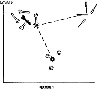
Figure 2.2 illustrates a hypothetical case where the

number of features available for recognition has been

reduced to two. The open shapes indicate feature

measurements made on each of several reference objects. The

solid shapes mark the centroids computed for each object

class. The unknown, designated

by

the

"X"

in Figure 2.2, is

identified

by

choosing the class whose centroid is the

closest.

Intuitively, the feature that has a smaller variance

(standard deviation) should contribute more to the decision

process. Therefore, a Mahalanobis distance is suggested, in

which each feature is weighted and the weight is the

reciprocal of standard deviation.

The Mahalanobis distance [CASH863 between an unknown

object and the i-th reference object class is defined as

Vn

/

U(k)

-R. (k) _\

z

FEATURE

2

W

/

\

\

FUTURE

1 [image:26.540.105.445.148.488.2]

where N is the number of

features,

_U(k) is the k-th feature

value of the unknown object, Ri(k) is the average k-th

feature value for the i-th reference object class and <r. _(k)

is the standard deviation of that class. Note that the U(k)

and Ri(k) values are normalized

by

the variance. In the

present _{work, a.}

(k) is set to 0.01 if it is less than 0.01.

We further extend the definition of Mahalanobis

distance to include the distance between two object classes

i and _j,

/n

/ _{Rj_} (k)

-R. (k) \:

' _k=l

\

o

(k) + o. (k)

/

\

=\"

I

1

_(2.6)

Note that

during

the calculation of Mahalanobis

distance,

only the average feature values and their

variances are needed. This leads to less stored data and a

much simplified computation.

Cash and Hatamian [CASH863 studied various

clssification techniques.

They

recommended the use of

Mahalanobis distance for its adequate recognition rate and

easy implementation. This study will use Mahalanobis

distance along with the nearest neighbor algorithm for

classification.

Other approaches, such as the

binary

decision tree

[AGIN803,

has been used for classification.

However,

we use

2.5. Simulation

by

Shape Generation

This study tried to bypass image _acquisition,

segmentation and edge detection.

Instead,

the digitized

edges of a shape were generated _{mathematically} and then

processed directly.

Hooper and Klinger proposed a similar idea [HOOP863

when

they

advocated that artificial pattern generation was a

useful technique for providing large banks of data that

could be used as test data for pattern recognition

experiments. The generated patterns were distorted under

control in this thesis to yield a wide variety of samples

that were different

from,

but similar _to, the original

pattern.

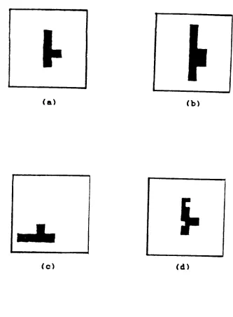
The distortions included linear stretching in either a

horizontal or vertical

direction,

rotation and relocation,

blurring

and random noise. Figures 2.3 and 2.4 present some

of the examples. Figure 2.3 gives an original image and its

stretched, relocated and noisy-added images. Figure 2.4

shows a curve before and after blurring.

2.6.

Summary

In this chapter, we have reviewed the hardware for the

actual robot vision systems. We also have reviewed how to

achieve edge extraction. However; edge extraction was

simulated in our system

by

mathematically generating

(a) _(b)

5-(c) (d)

Figure 2.3. Examples of various distortion schemes.

(a) original

(b) vertical _stretching

(c) rotation and relocation

[image:29.540.121.454.97.549.2]

BB BB

f

"V

1* BB

B

1

1

r

1

1

B^B

!"

V

av

"6

P' _B

B

B B as BB

B

1

jr

-1

L

B 1

T

B

B MB B BBB

r

B

B B B

V

B

8"

B

J-r

(>

(b)

(0

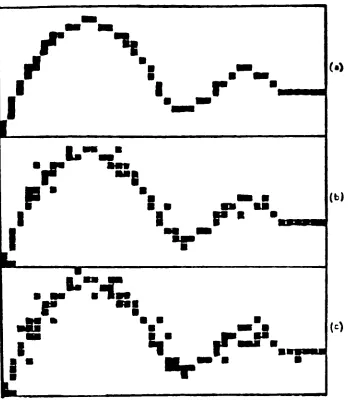
Figure 2.4. (a) the original digitized curve,

(b) the same curve after

blurring by

_adding 10% of the cells adjacent to the _curve,

(c) the result of

blurring

by

adding 20% of the [image:30.540.102.451.76.486.2]

Two major pattern recognition approaches, template

matching and feature extraction were

discussed,

_{but only} the

latter was considered suitable for our purpose. Invariant

moments are useful and were chosen as part of the features

in the pool.

Reduction the number of features can improve

recognition speed. We thus have studied two techniques to

automatically select useful features. One technique is to

eliminate redundant features and the other technique is to

pick a

feature,

for a pair of object _classes, with high

discrimination ability.

Identification was achieved

by

_using the nearest

neighbor classification algorithm. A Mahalanobis distance

was introduced and discussed. This distance can be

calculated between two object classes or between an unknown

CHAPTER 3

IMPLEMENTATION

3.1. System Overview

In this chapter, we describe the implementation of

image simulation and

digitization,

feature extraction, and

unknown identification in our system.

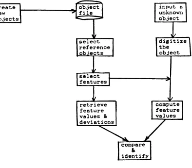
Figure 3.1 shows an overall system data flow diagram.

A new object and _many variations can be created _any time and

stored in the object file. The digitized image of an unknown

is generated mathematically. The stored feature values and

the standard deviations of objects of interest can be

retrieved when needed.

The task of recognition is restricted to _associating an

unknown with one of the selected reference objects. The

unknown is classified

by

comparing feature values of the

unknown to those of references. Classification is achieved

by

the nearest neighbor algorithm.

There are 12 features currently stored in our feature

pool. We have derived two rules for selecting an effective

feature subset. The system automatically does the selection.

Many

other flow charts are provided to show the details

of our implementation. Our system hardware and software are

Create

new

objects

select

reference

objects

select

features

retrieve

feature

values &

deviations

input a

unknown

object

digitize the

object

_*: compute

feature

values

[image:33.540.85.479.145.491.2]

3.2. Simulated Digitization

Digitization and edge extraction are two important

processes in robot vision. This thesis describes a system

that simulates the results from these processes and

mathematically generates the digitized edges of a shape. The

shape undergoes a series of translations, rotations,

scaling, and controlled distortions to form a class of

similar images.

In this study, we have limited the system to

binary

images.

3.2.1. Shape generation

Here,

we discuss how to generate an edge

extracted"

image.

The user first needs to decide the size of an object

and then plot the object on graph paper. The coordinates of

key

points of that object then can be obtained. We believe

that any digitized curve can be represented

by

a series of

line segments, although some line segments may be short.

For instance, a triangle is represented

by

the

coordinates of its three vertices. A line segment is defined

by

two points. Then a linear equation y=ax+b can be

determined, and the projections of this line segment on a

given grid can be calculated. The projections often will not

fall precisely on individual pixels, but the nearest pixels

to the projections will be turned "on". The mathematics here

perform this

digitization

task. An example is shown in

Figure 3.2.

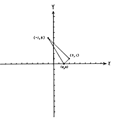
As shown in Figure

3.3,

for a _{triangle with three}

vertices

(2,0),

(3,1) and (-1,5). four points need to be

specified,

(2,0),

(3,1),

(-1,5) and

(2,0),

to indicate that

it is a closed curve. Note that the first and the last

points are the same.

Our system was designed in such a _way that it

automatically digitizes three line segments, (2,0) to (3,1),

(3,1) to (-1,5) and (-1,5) to (2,0).

We also wrote a procedure _{for generating} a digitized

circle, which is defined

by

a center coordinate and a

radius, based on Bresenham's circle algorithm [BRES773.

The

following

shapes will be examined

by

our system:

?,

?,

A,

^3,

O,

,

Jo], O,

<2>,

<&,

in which,

(q\

simulates a washer,

[OJ

and

Sq\

represent

nuts, and others are simple geometrical shapes.

3.2.2. Effect of Grid Size

One typical goal for a user of our system would be to

study the effect of camera resolution. This can be simulated

by

changing the grid size. This system was designed such

that digitization can be performed at three grid sizes,

Y

Figure 3.2. Digitization of a line segment.

(-!>*)

i . . i i i j

(3,l>

\s i 11 i i >. Y

(2,0)

[image:37.540.92.474.131.535.2]

system will scale _up (or down) the coordinates of those

key

points accordingly and then perform digitization.

Objects are often _easy to classify at a higher

resolution.

However,

_this benefit may diminish rapidly

beyond a certain _limit. This simulation can

help

the user to

determine a proper cost-effective resolution

by

_allowing him

to experiment with different resolutions and object sizes.

3.2.3.

Translation,

Rotation and

Scaling

When the pictures of an object are taken at various

locations,

orientations and camera-to-object

distances,

the

results of digitization are all different.

Therefore,

this

system provides translation, rotation and scaling operations

to perform these simulation tasks.

By

_performing various

transformations, a series of similar feature values will be

generated, which, along with those from original and other

controlled distortions, are considered to

belong

to the

same class. An average value and standard deviation for that

class then can be determined.

3.2.4. Controlled Distortion

Distortion operations are used to simulate device

inaccuracy. For instance, a circle may be distorted slightly

to become an ellipse, and the edges may be noisy. In this

system, an object can be shortened along the x direction

before it is digitized.

Blurring

is simulated

by

using a random number

between a shape and a _grid, a small

(e.g.,

-2 to 2 for a

grid size of 64x64) random number is added to the calculated

coordinates so that an

"on"

pixel may be shifted a few

positions in the x and/or _y directions.

The extent of x-axis compression (or elongation) and

pixel relocation in our system are controlled

by

two

parameters that are

temporarily

set at 5% and

i2/64,

respectively, in our controlled distortion. Comparisons

between the feature values of undistorted and distorted

shapes also give us some idea of the effect of distortion on

various feature values. For instance, if feature values

change a lot with single axis compression, we _may have to

select an acquisition device that has a smaller

compression/elongation distortion.

This system is aimed at simulating a real robot vision

system. For a real vision system, the extent of distortions

can be determined experimentally. The parameters used

by

our

system for controlling distortions then can be re-set

easily.

3.3. Classification

by

Feature Extraction

We intend to identify randomly oriented but well

separated objects on a conveyor belt. Based on the arguments

given in Section 2.4.1 and 2.4.2, the feature extraction

method of feature extraction is used in this study for

classification.

There are twelve features in our current feature pool.

In this section, we show how these feature values are

computed. Two rules to select an effective subset of

features are also _discussed.

3.3.1. Feature Pool

Our system is limited to simulating robotic visual

inspection and classification tasks. It is assumed that the

objects to be inspected are isolated and _randomly oriented.

In addition, the object _may not be at an exact position

under the camera. As a result, the selected features should

be independent of position, orientation, and size.

As an _aside, we understand that size-dependent

features can be useful.

By

using these

features,

for

example, printed upper case characters can be differentiated

easily from lower case ones. Our intent in using

size-independent features is that someday we hope this system

can be used to examine hand written characters of which the

sizes often vary. As a result, the size independent features

are especially useful for hand written characters.

Orientation dependent features are also useful in the

assembly of machine parts, since parts often need to be

properly aligned. The reason not to use orientation

dependent features is to avoid time consuming rotation

This system can be modified _easily to include size

and/or orintation dependent features

by

simply adding such

features to the feature pool. The

following

are the features

used in our system. This list could be expanded _easily if

desired.

F^a.ur._JL

(Rmax/Rav),

where Rmax is the longest distance ("radius") from

centroid to any

"on"

pixel and Rav is the average

distance from centroid to all

"on"

pixels. Note that

Rmax may be off

by

a lot if there is random noise.

This problem can be lessened

by

taking the average

distance for the 5% most remote

"on"

pixels, instead of

a single most remote

"on"

pixel, as Rmax.

Fjejanr_!5L_2.

(Rmin/Rav),

where Rmin is the shortest distance from centroid to

any

"on"

pixel. To lessen the effects of _noise, one _may

also take Rmin as the average distance for the nearest

5% "on" pixels from centroid.

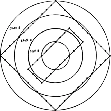
Feature 3 fraction of

"on"

pixels in cicular shell 1 as

shown in Figure 3.4. The radius for the outermost

circle is Rmax. A

"shell"

is defined as the area

between two neighboring circles.

Feature 4 fraction of

"on"

pixels in shell 2.

Feature 5 fraction of

"on"

pixels in shell 3.

Figure 3.4. Example for the computation of features

[image:42.540.55.491.118.551.2]

the radii. The total number of

"on"

pixels for both

rectangles is 72. The fraction of

"on"

pixels in shell 1 is

0.39 (28/72), which is the value of feature 3.

Similarly,

the values of feature 4 and 5 are 0.39 (28/72) and 0.11

(8/72), respectively. Note that the fraction of

"on"

pixels

in the innermost shell is not

included,

since it is

redundant to the other 3 shells.

Features 3 to 5 are proposed because it is obvious that

their values are independent of _orientation, size and

position.

They

can be considered as discrete

density

funtions,

where the digitized image is divided here into

four disjoint circular shells. It is reasonable to assume

that the number of shells can be increased if a grid size

greater than 64x64 is used.

Features 6 to 12 the 7 invariant moments derived

by

Hu

[HU623 are the choices and the formulas for computing

invariant moments are shown in Table 2.1.

Currently, there are a total of twelve features in our

Feature

number

Formula

_for

computing feature value

1 _{Rmax / Rav}

2 _{Rmin / Rav}

3

Fraction

_of "on"

pixels in shell 1 (Fig. 3. 4)

4

Fraction

_of "on"

pixels in shell 2 (Fig. 3. 4)

5 _{Fraction of} "on"

pixels in shell 3 (Fig. 3. 4)

6 _{1st invariant moment (Table}

2.1)

7 2nd invariant moment _(Table 2.1)

8 3rd invariant moment (Table 2.1)

9 4th invariant moment (Table 2.1)

10 5th invariant moment (Table 2.1)

11 6th invariant moment (Table 2.1)

12 7th invariant moment (Table 2.1)

Table 3.1. Features in our feature pool.

3.3.2. Feature Selection

For the recognition of some given objects, one _may not

need all the features in the feature pool. The problem is to

develop

a systematic _way to select an optimum subset of

features that can achieve both adequate

discrimination

and

high speed recognition. We have derived two selection rules

from the algorithms described in section

2.4.3,

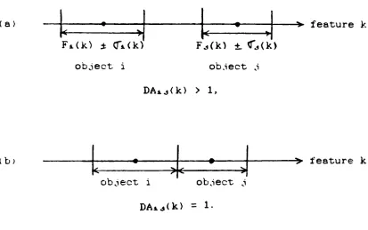
and both

By.le_JL.

Choose the feature with good discrimination ability when the feature is used alone.

As shown in Figure

3.5a,

the discrimination ability of

feature k for object classes i and j is defined as

('i

(k)

-F . (k)l

DA (k) =

_\_I

I

L-

(3.1)

J

o. (k) + a . (k)

i 1

where F*(k) is the k-th feature value for object class _i, and ^(k) is the corresponding standard deviation. In the

present study, a. (k) or a. (k) is set to 0.01 if it is less

than 0. 01.

Comparing

with Equation (2.6), the above definition is, in

fact,

a one-feature Mahalanobis distance. For a given

feature,

when the ranges of feature values of two object classes touch each other as shown in Figure

3.5b,

the discrimination ability for that feature will be unity.

Conceptually, one may say that a feature is statistically

"likely"

to differentiate two objects if its corresponding

discrimination ability is greater than unity.

In order to be more specific, let us assume that the distribution of feature values of an object in various states is a bell shaped normal function CDUDA73] . One then

can calculate the probability of occurences of a feature

(a)

<b>

F.(k) 0\<k) object i

Fj(k) +

Cj(k>

object j

DAj(k) > 1,

object i object

DA*.<k) =

1--v feature k

-> feature k

Figure 3.5. Discrimination abilities of feature k for

[image:46.540.66.479.232.491.2]

Range

Probability

mean feature value +/- ₁ o _68.27%

mean feature value

+/-2 a 95.45%

mean feature value +/- ₃

o 99.73%

Table 3.2.

Probability

of occurence for a feature value

to be within a range.

Armed with the information in Table

3.2,

one can

further calculate the probability of successful

discrimination

by

feature k for object classes i and j at

given Dtj(k) values. The results are shown in the table

below.

DtJ(k) value Successful discrimination

1 70.79%*

2 95.50%

3 99.73%

*

70.79% = _(0.6827 + 0. 5*( 1-0. 6827)

)2,

where probability of

object i occurs inside one standard deviation from its mean

=

0.6827,

and probabilty of object i occurs outside one

standard deviation from its mean but away from object j

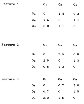
In order to better explain our _method, a hypothetical

example is given in Table 3.4 which _{includes 3 objects and 3}

features.

Feature 1 Oi Oa Oa

d 0 1.5 0.3

0* 1.5 0 1. 1

Oa 0.3 1. 1 0

Feature 2 0i 0s

Ox 0 2.5 0.8

Oa 2.5 0 1.3

Oa 0.8 1.3 0

Feature 3 Ox Oa Oa

Ox 0 0.7 3.0

0* 0.7 0 1.5

Oa 3.0 1.5 0

Table 3.4. Discrimination abilities

by

each feature

among 3 object classes.

Based on Table

3.4,

for

differentiating

Oa. from

Oa,

feature 2 is the best choice; for Ox and

Oa,

feature 3 is [image:48.540.88.406.151.548.2]

result, features 2 and 3 should be chosen as a subset for

classification. Note that the user can always include

additional features to the selected feature sub-set for

improved accuracy, but with a compromise in speed.

In our current _study, if the best feature provides a

discrimination ability less than

2,

then the next best one

also will be selected. For the object pair 2 and 3 in Table

3.4,

both features 3 and 2 are selected since neither of the

features has a discrimination ability greater than 2.

What

if,

for a pair of _objects, no feature with

discrimination ability greater than unity can be found? In

such a _case, it is always difficult to discriminate between

the object pair. It is thus advised to look for a better

feature outside the current feature pool.

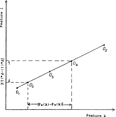
Rule 2 If two features are redundant for given reference

objects, one of them is deleted.

An example is illustrated in Figure

3.6,

where 5

objects are plotted in a 2-dimensional feature space and all

objects fall onto a straight line. This means that

F(k)-Fj(k) is proportional to F*.( 1)-Fj( 1) for any object

pair,ij. This also means that if an object pair can be

discriminated

by

feature

k,

it also can be discriminated

by

feature 1. As a result, one of these features can be

i-i

P

a)

a) fx,

i

k

|F(k)-F*(k)|

>

J

_>

Feature k

[image:50.540.77.453.130.507.2]

n n n. n

abilities,^

Dj(k)

andtL

D*.j(l),

_{which represent the}

' _V(j<i) * 3<j<i)

overall

discrimination

abilities

by

feature k and

1,

respectively. The feature with a smaller sum will be

deleted.

As a _summary,

Overall discrimination ability

by

feature k

= _DA(k)

n

= I

i

n

I

j (j

<

i)

D.j(k) (3.2)

We have explained the fact that 2 features are

considered redundant if the objects fall on a straight line

in the 2-dimensional feature space.

But,

how can a computer

tell if the objects are on the same line? This can be easily

achieved

by

the method of linear regression. All the points

are fitted to a straight line and the correlation

coefficient, r , are computed

by

the

following

equation

[FREU843:

r =

n _{( Ixy)} ( x) ( s y)

yjn ( XX2)

-( X x)2

->Jn( XV2) - (y)2

(3.3)

where n is the number of points (or objects) and x is the

sum of all x coordinates. The definitions for xy, Sxy, ix2

ry2are obvious.

points fall exactly onto a straight line. At r =

0,

_the

points can not be approximated at all

by

a straight line.

In this section, we first defined the discrimination

ability

by

a feature for any object pair. With this

definition,

it became easier to explain the redundancy of

feature pairs.

However,

in the implementation of our _system, we first

examine all feature pairs for redundancy and one feature is

deleted in a redundant feature pair.

Presently,

one feature

is deleted if r > 0.95. As a rule,

delete feature k if r > 0. 95 & DA( 1) > DA(k),

delete feature 1 if r > 0.95 & DA(k) > DA(1). (3.4)

After redundancy is removed, we then use the

discrimination ability to select the most discriminating

feature for each object pair.

The system deals with one feature or one feature pair

at a time. It avoids handling a large number of features

simultaneously. Our approach saves time, and the results are

good.

3.3.3. Classification

With the selected feature subset, the Mahalanobis

distance between an unknown and each chosen reference object

along with the Mahalanobis distances are used for

classification.

3.4. Flow Charts of Implementation

In the

beginning

of this chapter, we presented a flow

chart to show the overall picture of our system. The chart

is shown in Figure 3.1.

Here,

we present five additional

flow charts to describe the details of our system

implementation.

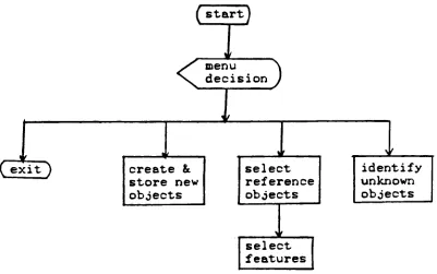
3.4.1. Hierarchical Process Diagram

Our system was designed to be menu driven. One of three

main paths can be selected

by

the user at one time.

They

are

(1) create and store objects, (2) select reference objects

to be compared and then select a feature subset, and (3)

identify

unknown objects.

A flow chart of the main menu is shown in Figure 3.7.

The details of each path are discussed in the succeeding

sections.

3.4.2. Create and Store Objects

This is an interactive system, in which the coordinates

of

key

points for an object are provided

by

the user

whenever the system prompts for them. The coordinates come

(

start)

<oenu

\

decision

J

exi

D

create &

store new

objects

select

reference

objects

identify

unknown

objects

select

features

[image:54.540.72.473.141.392.2]

(start

)

N>0

prompt for Cx,y)

positions of

centers and radii

prompt for positions

of

key

points

J

prompt for grid

size

1

|digitize

the object

J.

|

plot the object

~\

{save to object pool

"1

examine the condition

for distortion

-><menuy.

scale _up Cdown) input _coordinates

save to feature

pool

compute mean _feature

values & deviations

calculate feature

value

{digitize

jthe

obJect|

re-compute the Input

feature values and their standard

deviations,

and _saving the

information in a disk file. The user _only needs to provide

coordinates at one grid size, and the system will examine

the object at several different grid sizes to study the

effects of camera resolution.

3.4.3. Select Reference Objects

Figure 3.9 gives the sequence in the selection of

reference objects for comparison with the unknown. First of

all, the user opens the object file on a disk and retrieves

the information about all saved objects. The system first

displays a list of object names from which the user can

select. It then displays the image of the object selected

for the user to confirm. After all the reference objects are

chosen, only their feature values and standard deviations

are used in the next step, which is to select an effective

feature subset.

3.4.4. Select a Feature Subset

The subset of features is automatically selected

by

the

system according to the rules explained in Section 3.3.2.

As shown in Figure

3.10,

the system provides information on

(a) the correlation coefficient of all feature pairs, and

(b) discrimination ability of _every feature for all object

pairs.

Later,

only the selected features are used for

(start)

jopen

object pooT

*ften,Q

display

object

table

I

enter object

index

1

digitize object 1

|

plot object

|

correct.

Yes

(Jo

save

key

points of

object to reference

object file

1

save feature values & deviation to

(

start"")

compute

correlation coefficient

delete

redundant

features

compute

discrimination

ability

select

effective

features

establish

feature

subset

^

menu

)

3.4.5.

Identify

Unknown Objects

Figure 3.11 shows the path for

identifying

unknown

objects. The information to plot the unknown object will be

prompted

by

the system. The system then displays an image of

the unknown object on the monitor for the user's

confirmation.

The system then computes the values of selected

features for the unknown object. These values are used to

calculate the Mahalanobis distance to each reference object

class in the selected feature space. The unknown then can be

identified based on the nearest neighbor classification

algorithm.

Along

with each identification, it is helpful to define

a confidence

level,

which is shown

below;

Confidence level is high if Da > 3 and Dx < _2,

Confidence level is low if Da < 1 or Dx >

3,

Condidence level is average otherwise. (3.4)

where Dx is the Mahalanobis distance from unknown to the

nearest reference object class and Da is the distance from

unknown to the next nearest reference object class. In

addition, if an unknown is identified with a reference

object class that has a short Mahalanobis distance ( < 1 )

to another reference object class, then the confidence level

(

start")

prompt for the

information of unknown object

periorm a

random

distortion

digitize &

display

object

No

compute

feature values

I

compute Mahanalobis distance to each

reference object

identify

unknown

give confidence level & a second guess

<

menu

)

Without

involving

_{rigorous mathematical derivations and}

based on the probabilities shown in Table

3.2,

one sees that

the probability of _mistakenly

finding

_{the unknown to be the}

second nearest object is no more than 0.27% when Da > 3. The

additional condition for a high confidence

level,

Dx <

2,

assures that the unknown is in the neighborhood of the

nearest reference object.

One also sees that the probability of _mistakenly

finding

the unknown to be the second nearest reference

object can be as high as 68.27% when Da < 1 and that the

probability of correctly

finding

the unknown to be its

nearest neighbor is less than 0.27% when Dx > 3.

Now,

we are

fully

prepared to

identify

unknown objects.

In some _cases, the system can

identify

an unknown with high

confidence. In other cases, the system makes identification

by

its best judgement, but also informs user that the

confidence level is low or average.

3.5. System Hardware and Software

The system runs on a super Turbo (10 MHz) IBM-XT

compatible computer with 640K

RAM,

a 30 MB

Seagate,

hard disk

and a 360K floppy drive. Our simulated shape recognition

program and related data files were installed on the hard

disk for fast access. A Seikosha dot matrix printer is used

language. The Turbo PASCAL compiler, version

4,

was _used,

and the line compile option was chosen.

A large _{memory, ~110K,} was needed to edit our program,

which could not be handled

by

the Turbo PASCAL editor. As a

result, a word _{processing program,} Microsoft WORD version

3.0,

was selected to do editing. WORD was also used to

produce this thesis manuscript.

3.6.

Summary

In this chapter, the discussion includes mathematcally

generating images and also ways of

implementing

controlled

distortions.

There are currently 12 features used

by

the system. For

a given object domain, the system can automatically choose

an effective feature subset for improved recognition speed.

Classification was done

by

the nearest neighbor

algorithm and the Mahalanobis distance was adopted.

Five flow charts were presented to show the

architecture of the system and the details of the

imp

1ementation.

The system hardware was described. The operating

CHAPTER 4

RESULTS AND DISCUSSION

In this chapter, we will discuss the variables

manipulated in

testing

our system and also the system's

performance. We have included 12 features, 10 different

objects, 4 types of

distortion,

and 3 grid sizes to

demonstrate various aspects of our work.

The objects, both with and without

distortions,

were

digitized mathematically. This was done to simulate image

sensing,

digitization,

and edge extraction processes in an

actual robot vision system.

Feature values and their standard deviations were

computed for all 12 features and 10 object classes.

Mahalanobis distances in the 12-dimensional feature space

between 10 object classes also were computed.

The effect of resolution is discussed

by

showing

results at 3 different grid sizes. Results also are shown to

explain the algorithms for selecting an effective feature

subset in a given object space. Our method avoids

handling

many features simutaneously.

First,

features were examined pairwise to determine

their redundancy, which was measured

by

the corresponding

redundancy and then _selecting the most

discriminating

features from the _remaining ones.

Finally,

an unknown at its randomly distorted state was

identified with one of the reference objects based on the

nearest neighbor classification algorithm.

4.1. Graphic Representation of Edge-Extracted Objects

Image sensing, digitization and edge-extraction

processes _usully are done

by

hardware in an actual robot

vision system. In this study, we tried to simulate the end

results of these processes

by

_{mathematically generating} the

edge-extracted images.

Ten geometric objects were included for demonstration.

Plots of some digitized objects with and without distortions

are shown in Figures 4.1 to 4.4. Four types of controlled

distortion and also the magnitude of distortions are

tabulated below.

4.1.1. Objects in the Object Pool

We have stored 10 simple geometric objects in our

object pool. These objects are listed in Table 4.1 and their

i _o

'? C'

y o

'-'

o

; 2 o

:u z<

*. <^i

. . .'_>. .

5,

. .o

,

o

< o

r '. '. 1 1 1 6. i

*

9

I '. '. '.

6

'. '. '. '. '. '.

o

V . .o

'-o. . . . .

-. . .

"

o

000000000600606000606000000600600

Figure 4.1. A isosceles triangle.

> . .000000000. . ,

.000 000.

.00...001

. .00 00

.0 c

. .0 o,

.0 o,

.0,

.0 o

. . .0 o...

. . .0. . o...

. .0 o. .

. .0 o. .

.0 o. .0 o. .0 o. o o o o o o o o o o o o

o . . o

o o

o o

.c>. ... ...o.

.0 o.

.0 o.

. .o c.

. .0. * o. .

...o o...

...o o...

. . . .O .u. . . .

,o o,

.0 o,

.0 .0

,0 o

,00... .oo.

[image:65.540.135.373.34.325.2]

.o,

.o. .oo... ...o.o

O...O. ... . .O . . . .C'O.oo. . . .

O.O. ..o.o. . . .o. . ....O...-.O..O.. . . . . I"l ^ ....>">. . . .o". . o.oo.

,...o.oo

ooo

:<o oo.o. . . . .C *. .O.OOOO . i ..0...0.oo .

oo... ..o.o.

.0.0. >o. .o

. .O ...O...O.

>o. ... ...00.o. . .

,0.0 ...O.O....

[image:66.540.150.411.163.437.2]

I. .0.. ... ..OO... .c ..0..0...

...u...o.. iO. ...OOOi t.0....*...*..0.>~<* , . . . .O o. .o. , 1 ..O O O...O.... 1

...o....oc.'Z"'... ...

... ...o... .00...

0.0

... ...0.0.0... . .O.aOO... ...

Figure 4.3. A distorted isosceles triangle.

blurring

by

pixel relocation: +2 to -2

x-axis compression: _none

rotation angle:

O,

>...o o...o.o..,

oc oo o,

'. ....O. ... ...r>..

.O. .O '. . .o. , .O

,-.O. .o . ,

o

-'

OO, .*_<

I-.o o

o o.o

..o.o... ...

...OO _OO

O O. . .

.o,

.i_'. o

.O.O.... . . .o

o...

o.o. ... ...o. .00 .o...

,O1

o... ,o. . . o... ,

.O..O.

1 .o. 00... .0.0.0. o...

'~i...O..O.O....O...i

o . .o.o

GO. .C , 00. .o. . . .o

o .,

Figure 4.4. A distorted circle.

blurring by

pixel relocation: ?2 to -2

x-axis compression: 5%

rotation angle: 51

[image:67.540.123.449.97.439.2]

Index

Object Name

1 Square

?

2

Rectangle

?

3 Isosceles Triangle

A

4 Right Triangle

^3

5 _Circle

O

6 Washer (Ring)

7 Nut (Circle in Square)

0

8 Hexagon

o

9 Nut (Circle in Hexagon)

<o>

10 _Asymmetric Shape

*33

Table 4.1. Objects in the Object Pool.

The coordinates of

key

points for these 10 objects in a

64x64 frame are shown in Table 4.2. Note that the objects do

not

fully

occupy the whole field of view. The system

automatically calculated the coordinates for 32x32 and 16x16

frames

by

multiplying all coordinates with factors 0.5 and

0.25,

respectively. The resulted numbers from multiplicaton [image:68.540.92.392.48.328.2]

Key

points Center

Object of lines of a circle & radius

1 (-20,20X20, 20X20,-20)

(-20,-20)(-20,20)

2 (-24, 12)(24, 12X24,-12)

(-24,-12X-24, 12)

3 (-16,-20X0,

20X16,

-20)

(-16,-20)

4 (-24,-4X24,10X24,-4)

(-24,-4)

5

6

(0,0), r = ₂₀

(0,0), rx = ₂₀

(0,0), ra = ₁₅

(0,0), r = 15 7 (-20,20X20,20X20,-20)

(-20, -20X-20,20)

8 (-10, 17X10, 17X20,0X10,-17)

(-10,-17X-20,0X-10,17)

9 (-10,17X10,17X20,0X10,-17) (0,0). r = ₁₂

(-10,-17X-20,0X-10,17)

10 (-24,10X26,22X26,-12) (16,0), r = 8

(-16,-12)(-24, 10)

As described in Section

3.4.3,

the object pool can be

expanded _easily

by

_{accessing the "Create and Store} Objects"

menu, which guides the user _step

by

_step through the process

of _creating a new object. Once a new object is created, it

will remain in the object pool until it is deleted and can

be retrieved whenever it is needed.

4.1.2. Digitized Images without Distortion

Figures 4.1 and 4.2 show the undistorted digitized

images of an isosceles triangle and a circle in the current

object pool. All images have a field of view of 64x64.

In the images, series of

"o"

characters represent edges

and the dots "." indicate pixels that are not part of an

edge. Since we chose to use text mode for printing the

objects, the line spacing has been re-set to be almost the

same as the spacing between characters on the same line. As

a result, a square looks like a square on paper.

4.1.3. Types of Distortion

The magnitude and number of each type of distortion,

for the current study, are listed in Table 4.3. There are a

total of 24 states(variations) for each object class. These

Magnitude Number*

of variations

+ 10% 3

5% 2

51

2

>n ~ 5% ₂

Type of Distortion

Change of size

x-axis compression

Rotation

Blurring by

pixel relocation ~ 5%

*

includes the undistorted state.

Table 4.3. Our controlled distortions.

With our system, the user can ask "what if"

questions.

For

instance,

what is the _ability to separate a rectangle

from a square if the x-axis compression is 20% instead of

5%,

or what will happen if the

blurring

effect becomes twice

as severe?

Each type of distortion is controlled

by

a single

parameter, which can be re-set _easily for the system. For a

real application, the distortion parameters should be

determined experimentally in order to closely simulate a

given robot vision system. These parameters can be

determined

by

repeatedly taking pictures of the same object.

4.1.4. Digitized Images with Distortions

Figures 4.3 and 4.4 show a distorted isosceles triangle

compression, which simulates the quality of images an actual

vision system might produce.

In Figure

4.4,

note that the number of x-axis pixels is

46 and the number of y-axis pixels is

49,

since the circle

is compressed along its x-axis.

4.2. Properties of the Objects in the Object Pool

Since our system recognizes objects

by

_using the method

of feature extraction, the first task is to compute various

feature values for each _object, and the second task is to

compute Mahalanobis distances among object classes in a

given feature space.

4.2.1. Average Feature Values and their Standard Deviations

Currently, there are 12 features employed in our

system. These features were defined in Section 3.3.1 and

stored in the feature pool. Feature values were computed for

24 variations of each object class. The average feature

values and their standard deviations, for 10 objects with a

grid size of 64x64, are shown in Table 4.4. The name of the

objects are shown in T