Feature extraction for robust physical
activity recognition
Jiadong Zhu
1, Rubén San‑Segundo
2*and José M. Pardo
2Introduction
With information obtained from sensors, computer based system can make more intelligent actions by adapting their behavior to the context conditions. These days, thanks to the development of multi-sensor networks, related research areas have increased rapidly. Among those areas, Human Activity Recognition (HAR) based on wearable sensors (accelerometer, gyroscope, magnetometer, etc.) has recently received lots of attention due to its large number of promising applications. One of the most interesting HAR applications is ubiquitous identification of physical activity. As we know, over-weighting is a general human problem as a result of a physical inactivity habit. A Lancet publication [1] estimates that physical inactivity causes 9% of all pre-mature deaths worldwide. By monitoring physical activity, we can help people to learn the calories they consumed or gained during the day in a much more precise way and
Abstract
This paper presents the development of a Human Activity Recognition (HAR) system that uses a network of nine inertial measurement units situated in different body parts. Every unit provides 3D (3‑dimension) acceleration, 3D angular velocity, 3D magnetic field orientation, and 4D quaternions. This system identifies 33 different physical activi‑ ties (walking, running, cycling, lateral elevation of arms, etc.). The system is composed of two main modules: a feature extractor for obtaining the most relevant characteristics from the inertial signals every second, and a machine learning algorithm for classifying between the different activities. This paper focuses on the feature extractor module, evaluating several types of features and proposing different normalization approaches. This paper also analyses the performance of every sensor included in the inertial meas‑ urement units. The main experiments have been done using a public available dataset named REALDISP Activity Recognition dataset. This dataset includes recordings from 17 subjects performing 33 different activities in three different scenarios. Final results demonstrate that the proposed HAR system significantly improves the classification accuracy compared to previous works on this dataset. For the best configuration, the system accuracy is 99.1%. This system has been also evaluated with the OPPORTUNITY dataset obtaining competitive results.
Keywords: Physical activity recognition, Human Activity Recognition, Feature extraction robustness, Type of sensor, Signal normalization, REALDISP Activity Recognition dataset, OPPORTUNITY dataset, Random Forest, Pattern recognition, Machine learning
Open Access
© The Author(s) 2017. This article is distributed under the terms of the Creative Commons Attribution 4.0 International License (http://creativecommons.org/licenses/by/4.0/), which permits unrestricted use, distribution, and reproduction in any medium, provided you give appropriate credit to the original author(s) and the source, provide a link to the Creative Commons license, and indicate if changes were made.
RESEARCH
encourage them to keep moving in order to prevent obesity along with the following health effects. Another delightful example is Home Care Monitoring, which allows disabled and elderly patients a continuous health and well-being supervision while they perform Activities of Daily Living (ADL) at home. For instance, when a patient falls, the system will alert a nurse, or, if the patient is doing a forbidden activity, the security staff [2].
The main contributions of this paper are the followings:
• We present an automatic HAR system for classifying 33 different physical activities.
• We analyze several feature extraction strategies to find the one with the best perfor-mance and robustness.
• We study the influence of the type of sensor on the system performance.
• We propose and evaluate several normalization strategies for dealing with the inter-user variability.
• We also evaluate and validate the system for Home Care Monitoring using an ADL dataset.
The results obtained in this paper significantly improve the accuracy obtained in pre-vious works on the same dataset.
This paper is organized as follows: Second section describes the background. Third section shows the system architecture in detail. Fourth section describes the dataset, the evaluation methods used in this work and the experimental results obtained with the proposed system. Sixth section summarizes the main conclusions.
Background
Human Activity Recognition systems can be categorized by machine learning algorithm and the type of sensor they used. Human activity recognition can be seen as a machine learning problem. To deal with this problem, the HAR system must extract features from sensor signals, generate a model for each activity, and classify next activities based on these models. In the literature, different machine learning solutions have been applied to the recognition of activities including Naive Bayes [3], Decision Trees [4], Support Vector Machines (SVMs) [5], Deep Neural Networks [6] and Hidden Markov Models (HMMs) [7]. In many works, several approaches have been compared using the WEKA learning toolkit [8] because it incorporates many machine learning algorithms. For example, Yang [9] compares the performance of several machine learning approaches: C4.5 Decision Trees, Naive Bayes, k-Nearest Neighbor, and Support Vector Machines. Kwapisz [10] compares three learning algorithms: logistic regression, J48, and multilayer perceptron. Not only supervised but also, unsupervised algorithms have been studied [11]. In many works [12], complex algorithms, like the Random Forest, have demon-strated a very good performance compared to simple classification algorithms. Because of this, the Random Forest has been the algorithm selected in this work.
activity can be characterized by defining the identity of sounds and their position in time sequence [15]. The main two disadvantages of ambient sensors are the require-ment of infrastructure (for example, installation of video cameras in the monitoring areas) and also, people do not always stay all their time in the same environment. These limitations can be overtaken by on-body sensors [16, 17]. Body-worn sensors add new possibilities to the human monitoring system [18]: they allow measuring body signals (e.g. physiological, motion, location) and they are portable, allowing user supervision at any location without the need of fixed infrastructure. Because of these benefits, several works have been developed using motion sensors in different body parts (e.g. waist, wrist, chest and thighs) and achieved good classification performance [19–22].
This work has been carried out using a public dataset: REALDISP Activity Recogni-tion dataset. This dataset contains recordings from 17 subjects performing 33 different gymnastic activities. This dataset has permitted several HAR works focused on different aspects. One interesting aspect has been the degradation suffered on the HAR accuracy depending on the sensor placement or the number of displacements (wrong placements) [23–25]. Other analyzed aspects have been the window size [24, 26], and the detection of activities transitions [27]. This paper contributes by analyzing several strategies for feature extraction and proposing several normalization approaches for dealing with the inter-user variability. As far as the authors know, this work reports the best HAR results using this dataset.
System architecture
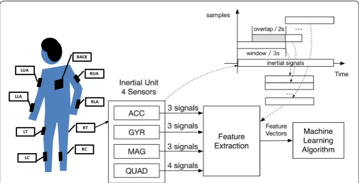
The proposed system architecture is shown in Fig. 1. It consists of two main modules: feature extraction and machine learning algorithm for activity classification. The inertial signals are recorded by 9 inertial measurement units. Every unit contains four sensors, accelerometer (ACC), gyroscope (GYR), magnetometer (MAG) and quaternion (QUAD)
BACK
RUA
RLA
RC RT LUA
LLA
LT
LC
sensor, which generate 13 inertial signals: in total, 117 inertial signals are processed. For more details, the reader can refer to [24].
Feature extraction
In the feature extraction module, the sample sequences from the inertial signals are grouped together in frames: fixed-width sliding windows of 3 s and 66% overlap (150 samples per frame with an overlap of 100 samples). For each frame, the system calcu-lates a feature vector, which makes it easier for the machine learning module to learn the internal characteristics behind raw signals. These features are traditional measures like the mean, correlation, Signal Magnitude Area (SMA) and auto regression coefficients, but also, advanced ones that will be described below. These features are computed from 117 signals obtained from nine measurement units. Taking the three accelerometer signals (X, Y, Z) as an example (similar signals are also considered for gyroscope, mag-netometer and quaternion sensor): in the time domain, the signals considered in this work are:
• XYZ (3 signals): Original accelerometer signals.
• Mag (1 signal): Magnitude signal computed from the previous three signals. This magnitude is computed as the square root of the sum of squared components (accel-erometer signals).
• Jerk-XYZ (3 signals): Jerk signals (derivative of the accelerometer signals) obtained from the original accelerometer signals.
• JerkMag (1 signal): Magnitude signal computed from the previous jerk signals (square root of the sum of squared components).
And in the frequency domain, the signals from the accelerometer sensor are:
• fXYZ (3 signals): Fast Fourier transforms (FFTs) from XYZ.
• fMag (1 signal): FFT from Mag.
• fJerk-XYZ (3 signals): FFTs from Jerk-XYZ.
• fJerkMag (1 signal): FFTs from JerkMag.
The set of features that were estimated from the time domain signals are:
• Mean value, standard deviation, median absolute deviation, minimum and maxi-mum values of the samples in a frame.
• Signal Magnitude Area: The normalized integral of the samples in a frame.
• Energy measure: Sum of the squares samples divided by the number of samples in a frame.
• Inter-quartile range: Variability measure obtained by dividing a data set into quartiles.
• Signal entropy.
• Auto-regression coefficients with Burg order equal to four correlation coefficients between two signals.
• Index of the frequency component with largest magnitude.
• Weighted average of the frequency components to obtain a mean frequency.
• Skewness and Kurtosis of the frequency domain signal.
• Energy of 6 equally spaced frequency bands within the 64 bins of the FFT.
Regarding the feature extraction complexity, we can comment that every feature is represented by 4 bytes, so every frame needs around 16 kB for storing a feature vector with all the features (4086 features) from all signals (117 signals from 9 measurement units). The features extractor has been implemented using Octave v.4.0.1. This module needs 12 min. for extracting the features in a whole session (around 18 min of physical exercise) using an Intel Core I7-4790 CPU at 3.6 GHz with 16 GB of RAM.
Machine learning algorithm
The machine learning algorithm module acts as a classifier. For this module, we have tried two popular algorithms (J48 decision tree and Random Forest) and found that the Random Forest algorithm [28] works better in this circumstance. In our preliminary experiments, it defeats the J48 decision tree algorithm by nearly 10% in accuracy. There-fore, the Random Forest algorithm is used in our following experiments.
The Random Forest algorithm creates several decision trees during training. In our experiments, the number of trees ranges from 40 to 95, and the number of nodes per tree goes from 15 to 87. These numbers varies strongly with the number of features con-sidered in the feature extractor. The algorithm for training the Random Forest model is:
Regarding the algorithm complexity, for building every decision tree the time com-plexity is O(m · n · log(n)), where n is the number of feature vectors in the training set, and m is the number of features in every feature vector. For building all the decision trees, the time complexity is O(t · m · n · log(n)), where t is the number of decision trees considered in the model.
For testing, the time complexity is O(t · n · m), where n is the number of feature vec-tors in the testing set, m is the number of features in every feature vector, and t is the number of decision trees considered in the model.
This work has been carried out using the Random Forest implementation included in the WEKA toolkit [8] (weka configuration weka.classifiers.trees.randomforest -I 100 -K 0 -S 1).
The training process needs less than 10 min for training the system using 16 sessions. The analysis and evaluation of 1 session (around 18 min of physical exercise) need less than 60 s, using an Intel Core I7-4790 CPU at 3.6 GHz with 16 GB of RAM.
Experiments
This section describes the experiments conducted in this work. In first and second sub-section, the main dataset and the evaluation methods used in this work are introduced. Third and fourth subsections shown the experiments carried out for the analysis of the type of sensor and the type of feature. In fifth subsection, the final results on the main dataset are given. At the end, sixth subsection includes an additional experiment on another HAR dataset—OPPORTUNITY dataset, using the same system.
REALDISP dataset
In this work, the HAR system has been mainly trained and tested using the REALDISP Activity Recognition dataset, available at the UCI Machine Learning Repository [24]. This dataset includes recordings from 17 subjects, seven females and ten males, with ages ranging from 22 to 37 years old. These recording include 13 inertial signals obtained from 9 on-body inertial measurement units located on different body parts. Each unit contains four sensors: an accelerometer, a gyroscope, a magnetometer and a quaternion sensor. Using these sensors, a 3D (3-dimension) linear acceleration, a 3D angular veloc-ity, a 3D magnetic field orientation and a 4D quaternions are sampled every 20 ms (50 Hz sample-rate). The experiment consisted in performing a complete set of exercises: 33 physical activities, including warm up, fitness and cool down activities (walking, jogging, cycling, jumping, etc.). One run-through of the exercises lasted 15–20 min. Each session was preceded by a preparation phase lasting around 30 min. This dataset also includes a Null-activity. This label has been assigned to other activities (different from the 33 activi-ties considered in this study), and also, the transitions between activiactivi-ties.
• Ideal-placement all sensors were placed by experts at their optimal place for classifi-cation. All the subjects recorded a session in these conditions (17 sessions).
• Self-placement every subject decides the positions of three sensors by themselves and the remaining sensors were situated by experts. The number of three is considered a reasonable estimate of the proportion of sensors that may be misplaced during the normal wearing. All the subjects recorded a session in these conditions (17 sessions).
• Mutual-placement where several displacements were intentionally introduced by experts. Three out of the 17 volunteers were recorded for mutual-displacement sce-nario (subjects 2, 5 and 15). These three subjects recorded one session for every sen-sor configuration: for the case in which four, five, six or even seven out of the nine sensors are misplaced.
Considering the size, the number of activities and the different placement scenarios, we think that the REALDISP dataset is an appropriate dataset to evaluate the perfor-mance of the proposed HAR system.
Evaluation methods
In this work, we apply two methods to evaluate the system performance. The first one is a tenfold random-partitioning cross-validation evaluation. This method consists of split-ting the whole database (with all subjects’ data) randomly into 10 equal parts (subsets). For every experiment, one subset is used for testing and the other nine for training, con-sidering a round-robin strategy. The final cross-validation result is the average along the 10 experiments. This is the method used in the original paper [24].
However, our hypothesis is that this method suffers the problem that the data in both training and testing could contain information from a same subject, so the machine learning algorithm can learn not only physical activity characteristics but also some subject-dependent ones. This aspect makes it hard to evaluate the system performance when facing a new subject. In order to verify this hypothesis, sect. “Evaluation methods” includes some experiments comparing both evaluation methods.
Therefore, we propose the second method, a subject-wise cross-validation. In this case, the same kind of cross-validation is done but on different subjects rather on auto-matically split parts: all data from the same user is considered for testing and the data from the remaining subjects for training. Since we have 17 subjects in the database, this experiment is repeated 17 times. The final experimental result is the average of accuracy and F-measure on all 17 sub-experiments weighted by the number of samples in every testing data.
In this work, we only use the tenfold cross-validation method to compare with our second evaluation method (“Evaluation methods”). The rest experiments are conducted with the subject-wise method.
In order to measure the statistical significance of the improvements, we apply the con-cept of Confidence Interval defined by Eq. 1 [29], P is the accuracy rate, and N is the amount of instances in the data set: more than 130,000 in the REALDISP dataset.
(1)
δ= ±1.96×
If the accuracy difference between two experiments is bigger than the confidence interval, this difference can be considered significant with a 95% of probability. In this paper, for all the experiments, the confidence interval is lower than 0.5%, so any differ-ence higher than this value, this differdiffer-ence can be considered as significant with a 95% a probability.
Data analysis
In this section, we first conduct some experiments for HAR system configuration tuning in order to analyze how the evaluation, the sensor type, or the feature type influences the system performance.
Evaluation method
This section includes the experiments considering the two different evaluation meth-ods. In these experiments, the setup is: ideal-placement, Null-activity removed (as in the original paper), and time-based features. The experimental results are shown in Table 1. From the results, we can clearly see that the result given by the random-partitioning method is significantly better than the subject-wise method: the accuracy (Acc%) differ-ence is 3.4% (99.1–95.5%) higher than the confiddiffer-ence interval, 0.5%.
This result supports the hypothesis stated in the previous section: in the random-part evaluation, training and testing subsets could contain information from a same subject and this characteristic produces better classification results. In the rest of the paper, we will only consider the subject-wise evaluation method (more challenging situation).
Type of sensor
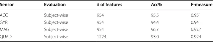
This section includes the experiments on different sensor types. In these experiments, the setup is: ideal-placement, Null-activity removed (as in the original paper), and time-based features. The experimental results are shown in Table 2. From the results, we can clearly see that the 3D magnetometer works best among the four types of sensor and the quaternion sensor performs the worst. The accuracy (Acc%) differences are statistically relevant because they are bigger than the confidence interval (0.5%).
Table 1 Experimental results depending on the evaluation method
Sensor Evaluation # of features Acc% F-measure
ACC Random‑part 954 99.1 0.991
ACC Subject‑wise 954 95.5 0.951
Table 2 Experimental results on type of sensor
Italic values indicate the best results in this experiment
Sensor Evaluation # of features Acc% F-measure
ACC Subject‑wise 954 95.5 0.951
GYR Subject‑wise 954 94.4 0.941
MAG Subject‑wise 954 96.3 0.952
Type of feature
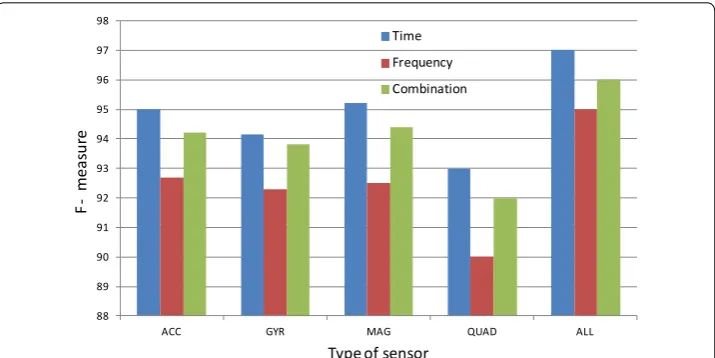
We also make a comparison on the performance of different kinds of features, more spe-cifically, temporal features and frequency features as described in “Feature extraction”. Same as the experiments on sensor types, here, we also consider the ideal-placement, removing the Null-activity. For the sake of confidence, we repeat the experiments with different types of sensor.
From the results shown in Fig. 2, it is obvious that the temporal features always beat the frequency features and their combination in the cases of all three sensor types. Therefore, we consider only the time-based features in the rest experiments.
As a conclusion, it is clear that using the signals from magnetometer and the time-based features is currently the best system configuration. By including all sensors, we obtain even higher system accuracy: 97.0%.
Normalization methods
When training and testing with different subjects, it is important to deal with the inter-user variability. In order to reduce this variability, we propose several normali-zation strategies. In this work, we evaluate six normalinormali-zation methods, considering two different places where this normalization is applied: before and after the feature extraction.
1. Mean removal: Subtract the mean value from each value in a feature or signal vector. 2. Z-Score: Mean removal first, and divide each value by its standard deviation.
3. Histogram equalization: Consider all the values in a gray-scale, and equalize its his-togram.
4. 0–1 mapping: Distribute all data to the 0–1 range.
5. Vector normalization: Divide each value in a vector with the vector’s magnitude. 6. Vector normalization with mean normalization: Vector normalization followed by
mean removal.
88 89 90 91 92 93 94 95 96 97 98
ACC GYR MAG QUAD ALL
F-me
as
ur
e
Type of sensor
Time Frequency Combination
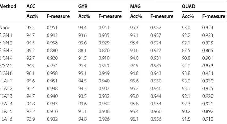
Note that in Table 3, SIGN_1 means normalization on signal data using method 1 and FEAT_1 means normalization on feature data (i.e. after feature extraction) using method 1. The results show that the vector normalization method (number 5) applied directly on the signal data outperforms all other methods. Thus, for the rest of the report, we use this normalization method before the feature extraction.
Final results and discussion
By applying the best experimental configuration described above, we conducted experi-ments using data from all signals and all sensors in all the three placement scenarios.
Ideal placement
Table 4 shows our final experimental results for the ideal placement scenario. After introducing the signal normalization method and considering all sensors, the system accuracy goes to 99.4%, a 2.4% improvement compared to the original paper (97%). This improvement is higher than the confidence interval (0.5%) so the difference is statisti-cally significant with a 95% of probability. It is important to notice that, in the original paper, the evaluation method was random-partitioning and, based on the results pre-sented in “Evaluation method”, the baseline accuracy would be even lower when using the subject-wise cross-validation method.
Another aspect to comment is regarding the Null-activity. In the first two rows of Table 4, the experiments are conducted without considering the Null-activity, in other words, it is a 33-class classification task. We truncated the Null-activity samples in order to make a fair comparison with the original paper. In this work, we have also done exper-iments including the Null-activity, which, in our opinion, is closer to a real situation. So, the problem now becomes more challenging: a 34-class classification task. Regarding the results shown in the third row of Table 4, our system still maintains a high performance when the Null-activity is included: the system only loses 0.3% accuracy (from 99.4 to 99.1%) showing a significant improvement (2.1%) respect to the baseline system (97%).
Table 3 Experimental results on normalization methods
Italic values indicate the best results in this experiment
Method ACC GYR MAG QUAD
Acc% F-measure Acc% F-measure Acc% F-measure Acc% F-measure
None 95.5 0.951 94.4 0.941 96.3 0.952 93.0 0.924
SIGN 1 94.7 0.943 93.6 0.935 96.1 0.957 92.2 0.923
SIGN 2 94.5 0.938 93.6 0.929 93.4 0.924 92.1 0.923
SIGN 3 89.2 0.880 88.1 0.870 93.6 0.927 87.5 0.865
SIGN 4 92.7 0.920 91.5 0.910 94.0 0.931 90.8 0.901
SIGN 5 96.4 0.961 95.4 0.950 97.9 0.976 94.1 0.939
SIGN 6 96.1 0.958 95.1 0.949 94.8 0.943 93.8 0.934
FEAT 1 95.6 0.951 94.5 0.940 95.6 0.950 93.0 0.930
FEAT 2 95.4 0.948 94.3 0.937 95.2 0.946 93.1 0.925
FEAT 3 94.7 0.940 93.5 0.932 95.0 0.944 92.1 0.920
FEAT 4 94.8 0.943 93.6 0.932 95.8 0.954 92.3 0.921
FEAT 5 92.2 0.916 91.1 0.908 96.4 0.960 90.2 0.892
Such low degradation is made possible due to the large number of features extracted and the suitable normalization method proposed in this paper.
Self and mutual placement
We repeat the previous experiments on the other two scenarios described in “ REALD-ISP dataset”: self-placement and mutual-placement. The results are presented in Table 5. In the first two columns, this table shows the type of data (or scenario where the data were recorded) used for training and testing the proposed system.
Regarding the self-placement scenario, this table shows 8.6% accuracy drop compared to the ideal-placement in the original paper (from 97.0 to 88.4%), but with our system, this reduction is lower than 0.5% (from 99.1 to 98.9%). When comparing these results to the original paper, there is a big improvement (more than 10%, from 88.4 to 98.9%) in the self-placement scenario. The new feature extraction module shows a very good robust-ness against different sensor placements.
For the mutual-placement scenario, the results are considerably low in both works (baseline and this paper) but the degradation obtained with the system proposed in this paper is considerably smaller compared to the baseline system: our system shows a bet-ter robustness. This degradation is different depending on the number of mis-displace-ments (4, 5, 6, and 7).
In these experiments, we have used the data recorded in the mutual scenario for train-ing and testtrain-ing the system. As we commented in “REALDISP dataset”, only three out of the 17 volunteers were recorded for mutual-displacement scenario so the amount of data
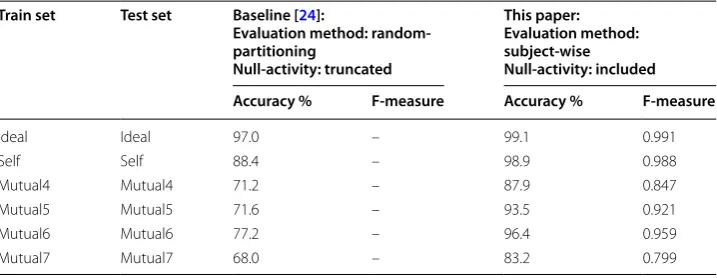
Table 4 Final experimental results considering the ideal placement scenario
System Accuracy % F-measure
Baseline [24]:
Evaluation method: random‑partitioning Null‑activity: truncated
97.0 –
This paper:
Evaluation method: subject‑wise Null‑activity: truncated
99.4 0.993
This paper:
Evaluation method: subject‑wise Null‑activity: included
99.1 0.991
Table 5 Final experimental result for self-placement and mutual-placement scenarios Train set Test set Baseline [24]:
Evaluation method: random- partitioning
Null-activity: truncated
This paper: Evaluation method: subject-wise Null-activity: included Accuracy % F-measure Accuracy % F-measure
Ideal Ideal 97.0 – 99.1 0.991
Self Self 88.4 – 98.9 0.988
Mutual4 Mutual4 71.2 – 87.9 0.847
Mutual5 Mutual5 71.6 – 93.5 0.921
Mutual6 Mutual6 77.2 – 96.4 0.959
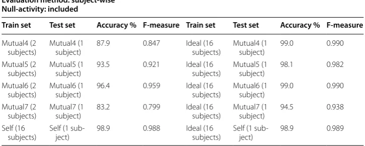
for training the system is very small (2 out of the 3 subjects recorded in this scenario). In order to analyze the influence of the amount of data, we repeat the same experiments but using the ideal-placement data for training the system. Although there is a mismatch in the conditions, the amount of available data for training would increase a lot (from 2 to 16 subjects). The experiments are shown in Table 6. In the “Train Set” and “Test Set” columns, we have also included the number of subjects considered for training and test-ing the system.
The results show that when being trained with ideal datasets and tested with mutual datasets, the system reaches a very good accuracy though the training and testing sets come from different placement scenarios. For example, for mutual4, the accuracy goes from 87.9 to 99.0% (the first row). These results support the hypothesis that the amount of data for training is an important factor in the system performance.
With the idea of cross-dataset experiment, we go further on the ideal-placement and self-placement scenarios (the last row in Table 6). As Table 6 shows, there is not a signifi-cant difference on the accuracy when testing with self-placement dataset and training with ideal or self placement (99.1 vs. 98.9%, difference lower than the confidence interval 0.5%). In this case, the amount of data available in ideal-placement and self-placement scenarios is the same.
System analysis in a new domain: home care monitoring
In the introduction, we commented two main applications of HAR: physical exercise monitoring and home care monitoring. The REALDISP dataset is focused on the first one: physical exercise monitoring. In order to verify the viability of the proposed system in a home care monitoring application, we have evaluated the best system configuration with another dataset: the OPPORTUNITY dataset for HAR from wearable, object, and ambient sensors [30]. The recordings include daily morning activities: getting up from the bed, preparing and having breakfast (a coffee and a salami sandwich) and clean-ing the kitchen latter. This dataset is a very popular HAR dataset on this research field. There is no constraining on the location or body posture in any of the scripted activities.
Table 6 Final experimental result for self-placement and mutual-placement scenarios: using ideal-placement for training
This paper:
Evaluation method: subject-wise Null-activity: included
Train set Test set Accuracy % F-measure Train set Test set Accuracy % F-measure
Mutual4 (2
subjects) Mutual4 (1 subject) 87.9 0.847 Ideal (16 subjects) Mutual4 (1 subject) 99.0 0.990 Mutual5 (2
subjects) Mutual5 (1 subject) 93.5 0.921 Ideal (16 subjects) Mutual5 (1 subject) 98.1 0.982 Mutual6 (2
subjects) Mutual6 (1 subject) 96.4 0.959 Ideal (16 subjects) Mutual6 (1 subject) 99.0 0.990 Mutual7 (2
subjects) Mutual7 (1 subject) 83.2 0.799 Ideal (16 subjects) Mutual7 (1 subject) 94.5 0.938 Self (16
OPPORTUNITY dataset
The OPPORTUNITY dataset contains data from four subjects, performing six different runs each of: ADL1–ADL5 and Drill. In the Drill run, subject must act in a predeter-mined activity sequence and, as for ADL1–ADL5, there is no restriction on the order and number of activities. For each subject, there is information from three types of sensors: body-worn sensors, object sensors and ambient sensors. The on-body sensors include 7 multi-sensor inertial measurement units with another 12 3D acceleration sen-sors: 145 signals in total. Since only body-worn sensors are concerned in the evaluation section of the original paper [31], the data from object and ambient sensors are trun-cated in the following experiments. In terms of activities or classes, this dataset has 3 different sets: 4 types of locomotion (high-level activities); 17 types of gesture (mid-level actions); and low-level actions to objects (which is ignored in this work).
Experiments on the OPPORTUNITY dataset
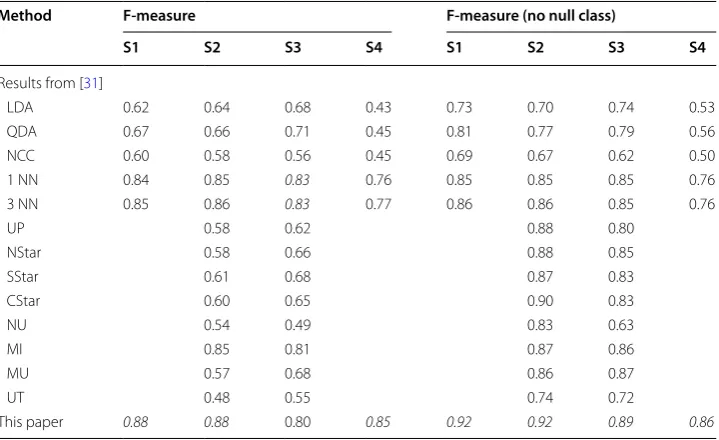
We retrain and evaluate our system using the same experimental setting as in the origi-nal paper [31]: using ADL2 and ADL3 from one subject as the testing set and use Drill, ADL1, ADL4 and ADL5 from the same subject as the training set. We conduct experi-ments in this configuration for all four subjects and in the two tasks: high-level loco-motion (Table 7) and mid-level gestures (Table 8). The first column shows the different proposed systems, and the best systems are remarked with bold font.
For the high-level locomotion task (Table 7), the system proposed in this paper obtains the best results for all subjects when the Null class is not considered (the 4 last columns). When including the Null class (the 4 first columns), we obtain the best results for all subjects except S3.
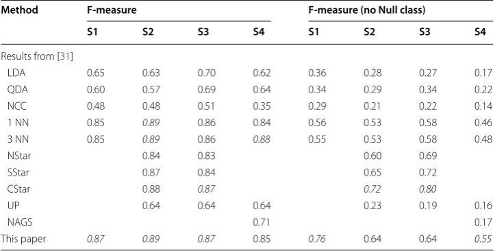
For the mid-level gesture task (Table 8), the system proposed in this paper obtains the best results for all subjects except S4 when the Null class is included (the 4 first
Table 7 Experimental results on the OPPORTUNITY dataset (high-level locomotion classi-fication)
Italic values indicate the best results in this experiment
Method F-measure F-measure (no null class)
S1 S2 S3 S4 S1 S2 S3 S4
Results from [31]
LDA 0.62 0.64 0.68 0.43 0.73 0.70 0.74 0.53
QDA 0.67 0.66 0.71 0.45 0.81 0.77 0.79 0.56
NCC 0.60 0.58 0.56 0.45 0.69 0.67 0.62 0.50
1 NN 0.84 0.85 0.83 0.76 0.85 0.85 0.85 0.76
3 NN 0.85 0.86 0.83 0.77 0.86 0.86 0.85 0.76
UP 0.58 0.62 0.88 0.80
NStar 0.58 0.66 0.88 0.85
SStar 0.61 0.68 0.87 0.83
CStar 0.60 0.65 0.90 0.83
NU 0.54 0.49 0.83 0.63
MI 0.85 0.81 0.87 0.86
MU 0.57 0.68 0.86 0.87
UT 0.48 0.55 0.74 0.72
columns). In conclusion, the proposed system is also a competitive solution for home care monitoring applications.
Conclusions
This paper has proposed a HAR system for classifying 33 different physical activities composed of two main modules: feature extraction and activity recognition modules.
The first contribution has been an analysis of several feature extraction strategies: time-based and frequency-based. The time-based features have provided better results compared to the frequency-based ones. This paper has also evaluated several normali-zation methods for reducing the degradation produced when training and testing with different users. Thanks to the new feature extraction module and the normalization strategy, the system has shown strong robustness when facing the Null-activity and dif-ferent placement scenarios, two vital aspects for real applications.
Regarding the type of sensor, the magnetometer signals have provided better discrimi-nation capability. The best results have been obtained when combining the information from all the sensors. In this case, the improvement is significant. The main experiments have been done on a public available dataset, REALDISP Activity Recognition dataset. Final results have exhibited that the proposed system largely improves the performance compared to previous works on the same dataset [24]. Under the best configuration, the accuracy reaches 99.1% and F-measure 0.991.
The proposed system has been also evaluated with another public dataset (OPPOR-TUNITY dataset) demonstrating competitive results (compared to previous work [31]) in two main tasks for home care monitoring: high-level locomotion and mid-level ges-ture classification.
Abbreviations
3D: 3‑dimension; ACC: accelerometer; ADL: Activities of Daily Living; GYR: gyroscope; HAR: Human Activity Recognition; HMM: Hidden Markov Model; MAG: magnetometer; QUAD: quaternion; SMA: Signal Magnitude Area; SVMs: Support Vector Machines.
Table 8 Experimental results on the OPPORTUNITY dataset (mid-level gesture classification)
Italic values indicate the best results in this experiment
Method F-measure F-measure (no Null class)
S1 S2 S3 S4 S1 S2 S3 S4
Results from [31]
LDA 0.65 0.63 0.70 0.62 0.36 0.28 0.27 0.17
QDA 0.60 0.57 0.69 0.64 0.34 0.29 0.34 0.22
NCC 0.48 0.48 0.51 0.35 0.29 0.21 0.22 0.14
1 NN 0.85 0.89 0.86 0.84 0.56 0.53 0.58 0.46
3 NN 0.85 0.89 0.86 0.88 0.55 0.53 0.58 0.48
NStar 0.84 0.83 0.60 0.69
SStar 0.87 0.84 0.65 0.72
CStar 0.88 0.87 0.72 0.80
UP 0.64 0.64 0.64 0.23 0.19 0.16
NAGS 0.71 0.17
Authors’ contributions
JZ has implemented the HAR and executed the experimental work. RSS has conceptualized the HAR system, supervised the experiments and revised the manuscript. JMP analyzed the results, provided feedback and revised the final manu‑ script. All authors read and approved the final manuscript.
Author details
1 School of Computer Science, Beijing University of Posts and Telecommunications, 10 Xitucheng Rd., Beijing 100876, China. 2 Speech Technology Group, E.T.S.I. Telecomunicación, Universidad Politécnica de Madrid, Ciudad Universitaria, Madrid 28040, Spain.
Acknowledgements
The authors would like to thank the UCI Machine Learning Repository and the researchers who kept the records and developed the REALDISP and OPPORTUNITY datasets.
Competing interests
The authors declare that they have no competing interests. Availability of data and materials
The datasets supporting the conclusions of this article are available in the UCI Machine Learning Repository, https:// archive.ics.uci.edu/ml/datasets.html. Regarding the software, the toolkit used for these experiments is WEKA (http:// www.cs.waikato.ac.nz/ml/weka/). This tool has been developed in Java for multi platform use. Weka is open‑source software issued under the GNU General Public License.
Funding
This work has been supported by China Scholarship Council scholarship and ASLP‑MULÁN (TIN2014‑54288‑C4‑1‑R) and NAVEGABLE (MICINN, DPI2014‑53525‑C3‑2‑R) projects.
Publisher’s Note
Springer Nature remains neutral with regard to jurisdictional claims in published maps and institutional affiliations.
Received: 15 November 2016 Accepted: 19 April 2017
References
1. Lee IM, Shiroma EJ, Lobelo F, Puska P, Blair SN, Katzmarzyk PT, Lancet Physical Activity Series Working Group et al (2012) Effect of physical inactivity on major noncommunicable diseases worldwide: an analysis of burden of disease and life expectancy. Lancet 380:219–229
2. Pavón J, Gómez‑Sanz J, Fernández‑Caballero A, Valencia‑Jiménez JJ (2007) Development of intelligent multisensor surveillance systems with agents. Robot Auton Syst 55:892–903
3. Jatoba LC, Grossmann U, Kunze C, Ottenbacher J, Stork W (2008) Context‑aware mobile health monitoring: evalua‑ tion of different pattern recognition methods for classification of physical activity. In: 2008 30th annual international conference of the IEEE engineering in medicine and biology society. IEEE, New York, pp 5250–5253
4. Maurer U, Smailagic A, Siewiorek DP, Deisher M (2006) Activity recognition and monitoring using multiple sen‑ sors on different body positions. In: International workshop on wearable and implantable body sensor networks (BSN’06). IEEE, New York
5. Anguita D, Ghio A, Oneto L, Parra X, Reyes‑Ortiz JL (2013) Energy efficient smartphone‑based activity recognition using fixed‑point arithmetic. J UCS 19:1295–1314
6. Ronao CA, Cho S (2016) Human activity recognition with smartphone sensors using deep learning neural networks. Expert Syst Appl 59:235–244
7. San‑Segundo R, Lorenzo‑Trueba J, Martínez‑González B, Pardo JM (2016) Segmenting human activities based on HMMs using smartphone inertial sensors. Pervasive Mob Comput 30:84–96
8. Holmes G, Donkin A, Witten IH (1994) Weka: a machine learning workbench. In: Proceedings of the 1994 Second Australian and New Zealand conference on intelligent information systems. IEEE, New York, pp 357–361 9. Yang J (2009) Toward physical activity diary: motion recognition using simple acceleration features with mobile
phones. In: Proceedings of the 1st international workshop on Interactive multimedia for consumer electronics. ACM, New York, pp 1–10
10. Kwapisz JR, Weiss GM, Moore SA (2011) Activity recognition using cell phone accelerometers. ACM SIGKDD Explor Newsl 12:74–82
11. Kwon Y, Kang K, Bae C (2014) Unsupervised learning for human activity recognition using smartphone sensors. Expert Syst Appl 41(14):6067–6074
12. Stisen A, Blunck H, Bhattacharya S, Prentow TS, Kjærgaard MB, Dey A, Sonne T, Jensen MM (2015) Smart devices are different: assessing and mitigating mobile sensing heterogeneities for activity recognition. In: Proceedings of the 13th ACM conference on embedded networked sensor systems. ACM, New York, pp 127–140
13. Poppe R (2010) A survey on vision‑based human action recognition. Image Vis Comput 28:976–990
14. Onofri L, Soda P, Pechenizkiy M, Iannello G (2016) A survey on using domain and contextual knowledge for human activity recognition in video streams. Expert Syst Appl 63(30):97–111
16. Lukowicz P, Ward JA, Junker H, Stäger M, Tröster G, Atrash A, Starner T (2004) Recognizing workshop activity using body worn microphones and accelerometers. In: International conference on pervasive computing. Springer, Heidelberg, pp 18–32
17. Karantonis DM, Narayanan MR, Mathie M, Lovell NH, Celler BG (2006) Implementation of a real‑time human move‑ ment classifier using a triaxial accelerometer for ambulatory monitoring. IEEE Trans Inf Technol Biomed 10:156–167 18. Bao L, Intille SS (2004) Activity recognition from user‑annotated acceleration data. In: International conference on
pervasive computing. Springer, Heidelberg, pp 1–17
19. Casale P, Pujol O, Radeva P (2011) Human activity recognition from accelerometer data using a wearable device. In: Iberian conference on pattern recognition and image analysis. Springer, Heidelberg, pp 289–296
20. Krishnan NC, Colbry D, Juillard C, Panchanathan S (2008) Real time human activity recognition using tri‑axial acceler‑ ometers. Sensors, signals and information processing workshop. pp 3337–3340
21. Ravi N, Dandekar N, Mysore P, Littman ML (2005) Activity recognition from accelerometer data. AAAI 5:1541–1546 22. Hanai Y, Nishimura J, Kuroda T (2009) Haar‑like filtering for human activity recognition using 3d accelerometer. In: Digital signal processing workshop and 5th IEEE signal processing education workshop, 2009. DSP/SPE 2009. IEEE 13th, IEEE, New York, pp 675–678
23. Banos O, Damas M, Pomares H, Rojas I (2013) Handling displacement effects in on‑body sensor‑based activity recognition. In: International workshop on ambient assisted living. Springer, Heidelberg, pp 80–87
24. Banos O, Toth MA, Damas M, Pomares H, Rojas I (2014) Dealing with the effects of sensor displacement in wearable activity recognition. Sensors 14:9995–10023
25. Punchoojit L, Hongwarittorrn N (2015). A comparative study on sensor displacement effect on realistic sensor dis‑ placement benchmark dataset. In: Recent advances in information and communication technology 2015. Springer, New York, pp 97–106
26. Banos O, Galvez JM, Damas M, Pomares H, Rojas I (2014) Window size impact in human activity recognition. Sensors 14:6474–6499
27. Reyes‑Ortiz JL, Oneto L, Samá A, Parra X, Anguita D (2016) Transition aware human activity recognition using smart‑ phones. Neurocomputing 171:754–767
28. Breiman L (2001) Random forests. Mach Learn 45:5–32
29. Cox DR, Hinkley DV (1974) Theoretical statistics. Chapman & Hall, London
30. Roggen D, Calatroni A, Rossi M, Holleczek T, Forster K, Tröster G, Lukowicz P, Bannach D, Pirkl G, Ferscha A, et al (2010) Collecting complex activity datasets in highly rich networked sensor environments. In: 2010 seventh international conference on networked sensing systems (INSS). IEEE, New York, pp 233–240