Using Cloud Computing for Scalable, Reproducible Experimentation

(1)

Using Cloud Computing for Scalable, Reproducible

Experimentation

Jonathan Klinginsmith

School of Informatics and Computing

Indiana University Bloomington, IN, USA

Judy Qiu

School of Informatics and Computing Indiana University

Bloomington, IN, USA

ABSTRACT

Whether it be data generated from genomic sequencers, tele-scopes, or other laboratory instruments, technology apparent in many scientific disciplines is generating data at rates never witnessed before. Scientists in the area of bioinformatics are among the many who perform inductive experiments and analyses on these data with the goal of answering scientific questions. These computationally demanding experiments and analyses have become a common occurrence, resulting in a shift in scientific discovery, and thus leading to the term eScience.

Reproducing controlled eScience experimental conditions is a challenging task. To reproduce an eScience experiment, the investigator must be able to recreate the original condi-tions, including operating system, software installations and configurations, and original data set. The challenge of repro-ducibility is compounded when the experiment must be run in a distributed manner.

In this work, we create a reproducible framework for the construction of large-scale computing environments on top of cloud computing infrastructures. We demonstrate how this framework can reduce the challenges of experimental reproducibility in large-scale eScience applications.

Categories and Subject Descriptors

H.4 [Information Systems Applications]: Miscella-neous

General Terms

Design, Performance

Keywords

Cloud Computing, eScience, Reproducibility

1. INTRODUCTION & MOTIVATION

Data-intensive science is considered part of a rela-tively new paradigm in the scientific discovery process [19]. The term eScience [27] has been coined to help explain the common themes and processes found in this new shift in scientific thought. One common need across

all domains of eScience research is to have an infrastruc-ture available with software configured to process large-scale data and perform simulations to produce scientific insight.

As a researcher investigating a scientific paper within a particular eScience domain, it can be challenging to reproduce the controlled conditions of the original au-thors’ experiments. To fully reproduce the experiments in the paper, one must have both the infrastructure and software configured in the same manner, as well as have access to the data used within the original experiment. In many cases, having access to all these items is not possible [42].

Even if the original data are not available, it should be a reasonable expectation within the scientific commu-nity for the experimental environment be reproducible. If the infrastructure setup and the software installation and configuration can be performed in a reproducible manner then eScience researchers, who are tradition-ally not system administrators, are much more enabled at replicating or extending the experiments being inves-tigated.

Therefore, in this work, we demonstrate through the use of cloud computing along with infrastructure and software automation the concept of scalable, reproducible experimentation is an achievable goal. To this end, this work enables eScience researchers to spend less time on the system administration processes of recreating a previous experiment and more time on enabling and ad-vancing scientific thought in his/her particular domain. Towards the goal of performing reproducible eScience experiments in the cloud, we demonstrate the follow-ing:

• The construction of computing framework, which enables scalable, reproducible experimentation.

(2)

2. BACKGROUND & RELATED WORK

2.1 Virtualization & Cloud Computing

Virtualization technology has opened the door to many advances in computing. A virtual machine (VM) [26] is a running instance of a computer where resources such as memory and central processing units (CPUs) are al-located through virtualization software. Cloud comput-ing has emerged in recent years because of advances in virtualization software. Companies such as Amazon, Google, and Microsoft provide services to customers for use of the virtual resources owned by them. The defi-nition of cloud computing has taken many forms in the academic community and industry. For this work, we use the definitions and terms discussed in [16].

Cloud computing refers to the software, platforms, and infrastructure services provided over the Internet as well as the data centers offering these services. The hardware and virtualization software running on top of this hardware is termed a cloud. Providers of cloud computing services offer application programming inter-faces (APIs) as means with which customers subscribe and interact. The lowest level of service available with a cloud is termedInfrastructure as a Service(IaaS). At this level, users provision virtual resources such as a VM or a virtual block storage device. We consider this the infrastructure layer whereabouts our framework inter-acts with the cloud.

2.2 Experimentation & Reproducibility

Four properties of good experimentation are outlined in [45]: 1) reproducibility, 2) extensibility, 3) revisabil-ity, and 4) applicability. An experiment exhibits the property ofreproducibility if another researcher is able to perform the experiment and produce the same result. The properties ofextensibilityandrevisability both dic-tate that changes to conditions and modifications must be possible for the experiment. Those changes may be necessary for future expandability or if a modifica-tion is needed for correcmodifica-tions to the original experiment. Lastly, experimental parameters must be of realistic in nature and resembling reworld conditions while al-lowing for changes to thus promoteapplicability.

The limits of reproducibility were reviewed in [22]. In this work, the author provides details of how stochas-tic methods, such as the use of genestochas-tic algorithms, can prevent an experiment from being fully reproducible. Moreover, the finite nature of floating point precision also limits numerical simulation reproducibility. Rela-tive to this work, our framework demonstrates that even if an exact numerical value cannot be reproduced, the experimental conditions and execution should be repro-ducible.

Experimental complexity and scalability are discussed in [21]. In order to answer more difficult scientific

ques-tions, both of these conditions must increase. There-fore, by advancing the processes for managing experi-ments will lead to improveexperi-ments in reproducibility and experimental integrity.

2.3 Appliances & Clusters

Several works [23, 28] have outlined how virtual ap-pliances can provide a reproducible environment for re-searchers. In [23], the authors propose reproducibil-ity as a two step process. First, by storing scientific datasets in the cloud more researchers have access to the data. Second, the authors introduce a concept called Whole System Snapshot Exchange (WSSE) where the entire computer system, including the operating sys-tem, is copied so that other researchers can fully repli-cate the in silico experiment. This same sentiment is shared in [28]. The author states that by provid-ing a pre-installed, pre-configured virtual machine the original “laboratory” is provided in tact for future re-searchers.

Our framework achieves the same outcome of repro-ducible computational experiments; however, only a generic, “golden” machine image is maintained within a cloud.

Then utilizing a configuration management tool, VMs are fully installed and configured software installation scripts at deployment run-time. Through this approach, we are able to use the same software installation and configuration scripts within the software layer in sepa-rate clouds. Moreover, using an automation approach to software installation and configuration management provides the ability to build scalable architectures in the cloud. The properties of scalability and elasticity have gained much of cloud computing’s attention, which has led to work in building virtual clusters.

A virtual cluster (VC) [25] is a set of VMs and any corresponding storage, which operate as a whole to cre-ate the presence of a single computational entity. The ability to quickly provision a VC within a cloud com-puting infrastructure is useful in many scenarios within eScience experiments. For example, a researcher can build the necessary environment closer to the data, es-pecially as more public datasets are being stored in the cloud [35]. Both [31, 15] discuss the how as the size of data sets grow, and if the construction of a VC can be performed in a straightforward manner, then it is pos-sible to move the computing infrastructure to the data. This is in contrast to moving the data to the location of a dedicated high performance computing (HPC) clus-ter, such as a research university’s supercomputer.

(3)

2.4 Genomic Sequencing in the Cloud

Scientists in the area of genomic sequencing have been performing research work in the cloud to provide the necessary scale in both computing power and storage [17]. The National Institutes of Health (NIH) announced in late March 2012 the 1000 Genomes Project [11] data are now available on the Amazon Cloud as a public data set [35]. There are many recent works on the use of cloud computing for bioinformatics and genomic se-quencing analyses [47, 40, 43].

2.5 Cloud Computing Technologies

Research work is also being performed tools, tech-nologies, and applications to create as well as manage cloud infrastructures. Eucalyptus [37] is an open-source cloud computing platform that provides IaaS capabili-ties. Using Eucalyptus, one can create a cloud with a compatible API to that of Amazon’s EC2 and S3. Dur-ing this research, our framework was implemented and tested both on Amazon as well as FutureGrid’s Euca-lyptus cloud.

There are several configuration management tools avail-able for use in automating software configurations and installations. Tools such as CFEngine [6] and Puppet [9] have been created to manage and configure infras-tructures and systems. In this work Chef [5] was chosen as one of the open source software products to aide in the framework implementation.

Other projects have built on top of these configu-ration management tools to help launch and configure independent VMs on IaaS clouds. One such tool is clou-dinit.d [20].

3. REPRODUCIBLE FRAMEWORK

3.1 Separation of Concerns

The foundation to our reproducible framework is the separation of interactions between an IaaS cloud com-puting infrastructure (the infrastructure layer) and the interactions of of a running virtual machine (the soft-ware layer). This separation of concerns allows for the reuse of software installation and configuration man-agement scripts between clouds. Moreover, any differ-ences in the IaaS cloud application programming inter-face (API) are handled at the infrastructure layer.

Figure 1 details how a client machine interacts with these two layers. For the infrastructure layer, the client interacts with the IaaS cloud provider’s API whereas within the software layer the client is executing com-mands directly on the running virtual machine.

3.2 Software layer

The software layer is the one in which a researcher in-teracts with the most often. This is where the scientists interacts with applications and the operating system.

client client VM

[image:3.612.334.535.54.107.2]

Software layer Infrastructure layer

Figure 1: Client interactions between the infrastructure and software layers.

Figure 2 provides details of the software layers neces-sary for a researcher to have a fully-configured running virtual machine to execute an experiment. Each layer within this running VM has a version associated with it.

The base layer is the operating system. Installed on the VM’s operating system layer are platform languages and software. For example, compiled languages such as C, C++, and Java as well as interpreted languages such as Perl, Python, and Ruby are foundational languages to many researchers work.

VM

OS Platform Software Application Software

[image:3.612.357.510.303.361.2]

Operating System Compliers Platform languages Platform software Domain-speciﬁc software and conﬁgurations

Figure 2: Operating system and software layers

Additionally, installed and configured on top of the running operating system, the VM has platform soft-ware and filesystems, which provide foundational com-ponents for distributed systems. HPC/HTC schedul-ing software, distributed file system software, and dis-tributed computing frameworks such as Hadoop [7] are all examples of platform technologies that domain-specific researchers use perform distributed computing experi-ments.

The final layer in the application stack is domain-specific software. Domain-domain-specific software is depen-dent on both the operating system and the platform technologies to be installed correctly.

When installing and configuration distributed sys-tems, application configuration files must be populated with values to allow machines to interact with one an-other. For example, when configuring a Condor [44] pool a file named condor config.local must be config-ured on each node of the cluster. This configuration file indicates which node in the pool is designated with the role of Central Manager. Reproducing an experiment that uses Condor as its scheduler must have its con-dor config.local file be populated with a different value than theCentral Managerof original experiment. Fig-ure 3 displays a Condor pool with an example of the

CONDOR_HOSTvariable populated in thecondor config.local

(4)

Central Manager Submit

cm

Condor

Execute

execute0001

Condor

Execute

executeXXXX

Condor

OS

OS OS

condor_conﬁg.local

CONDOR_HOST= cm

Figure 3: Condor pool with configured

con-dor config.local file

3.3 Framework Implementation

To implement the framework, two equivalent machine images were created. The first, a Eucalyptus Machine Image (EMI) was created in FutureGrid’s Eucalyptus cloud. The second, an Amazon Machine Image (AMI) was created in Amazon Web Service’s cloud. The fol-lowing steps were performed in each cloud to make the software layer consistent between the clouds.

• Launched a base CentOS 5.8 machine image (MI).

• Installed software configuration management open source software (specifically, thechef-client ver-sion 0.10.10).

[image:4.612.368.504.55.124.2]

• Registered the new machine image, which is con-sidered the “golden” machine image within that cloud.

Figure 4 provides a visual representation of the two machine images created in separate IaaS cloud.

EMI

OS

chef-client FutureGrid Eucalyptus

AMI

OS chef-client

Amazon

Figure 4: Equivalent machine images (MI) were built in IaaS separate clouds.

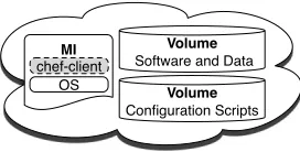
As opposed to storing fully configured virtual appli-ances in the cloud, we store several other persistent ob-jects that can be used to recreate the entire environ-ment. Figure 5 presents the three objects that are per-sisted in the cloud: 1) the “golden” machine images, 2) a volume containing the software source code (e.g., tar.gz files) and packages (e.g., RPMs), and 3) the software installation and configuration management scripts.

Figure 6 demonstrates how the persistent objects are used to reproduce eScience environments at scale. The volume storing the software source code, software pack-ages, and any data is attached to a deployment web

Volume

Software and Data

Volume

Conﬁguration Scripts

MI

[image:4.612.65.307.60.171.2]

OS chef-client

Figure 5: Persistent objects stored in the cloud.

server. This web server distributes the software to all of the running virtual machines. The second server hosts the scripts for installing and configuring these specific versions of software. This is the Chef server. There-fore, a snapshot of a scalable eScience application is persisted in the software artifacts and deployment in-stallation and configuration scripts stored through this framework. In the next section we use the implemen-tation of this framework to test both scalability and reproducibility.

Volume

Software and Data

VM

Web Server

VM

Chef Server

Volume

Conﬁguration Scripts

Each VM downloads versioned software and conﬁguration scripts

eScience VM Conﬁgured

Software

OS eScience VM

Conﬁgured Software

OS

eScience VM Conﬁgured

Software

[image:4.612.326.557.305.467.2]

OS

Figure 6: Chef server and software web server install and configure VMs.

4. EXPERIMENTS

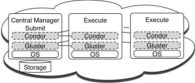
4.1 Scalability

[image:4.612.98.247.460.535.2]

(5)

Storage Central Manager

Submit Condor Gluster

Execute

Condor Gluster

... Execute Condor Gluster OS

[image:5.612.75.271.57.141.2]

OS OS

Figure 7: Scalability tests created a Condor pool.

The bottom chart begins to investigate the reasons for the additional deployment time. A result of creat-ing a “golden” image (with no pre-configured software), is that each individual node must download, install, and configure software at deployment run-time. The re-sult of this on-the-fly configuration is longer deployment times as the cluster size increases. Specifically because the software must be transferred over the cloud’s net-work from the web deployment server to each individual node.

For clusters of size 10, the deployment on average takes just over 40 seconds whereas for a 100 node clus-ter the average deployment for a node is around 120 seconds. The second chart in Figure 8 presents the to-tal received network traffic of the 100 execute nodes during a deployment. As witnessed by the large spikes, there are seconds during the deployment (around the 70 second mark, 80 second mark, and 120 second mark) where as a whole, the entire pool is receiving over 200 MB of software.

10 25 50 100

0 20 40 60 80 100 120 140 160

Tim

e (

se

co

nd

s)

Build Run Times per Cluster Size

0 20 40 60_{Time (seconds)}80 100 120 140 0

50 100 150 200 250

Re

ce

ive

d Da

ta

(M

B)

Network Traffic Received per Second - 100 Nodes

Figure 8: Node deployment times and network traffic received

Another item of note in Figure 8 is the larger standard deviation among the three tests of deployment 100 node clusters. Figure 9 delves into the details of one 100 node deployment.

The individual deployment times for each of the 100 nodes is presented in the top graph of Figure 9. The length of the horizontal lines provides the total run time for that particular node’s deployment. Some of the first execute nodes begin completing their deploy-ment as quickly as 80 seconds whereas the last nodes to complete take up to 70 seconds longer. This chart demonstrates why there is a larger standard deviation for the 100 node deployments.

The second chart in Figure 9 demonstrates when the Condor central manager recognizes the execute host has been registered in the Condor pool. The Condor instal-lation is the last step in the node deployment process because all other software needs to be configured be-fore the scheduler is to be enabled on the execute node. Therefore, this second chart provides another view into how many nodes have completed their deployment. One can see the association between the deployment comple-tion time and the Condor central manager registering a new execute node in the pool. This bottom chart demonstrates the elasticity or cloud-bursting capability of the cloud. In this particular case, a 100 node cluster has been created in 150 seconds.

0 20 40 60 80 100 120 140 0

20 40 60 80 100

No

de

Nu

mb

er

Node Deployment Time - 100 Nodes

0 20 40 60_{Time (seconds)}80 100 120 140 0

20 40 60 80 100

No

de

s R

eg

iste

red

in

Po

[image:5.612.328.552.346.524.2]

ol Condor Execute Nodes in Pool

Figure 9: Individual deployments times and Condor node counts.

[image:5.612.65.291.439.618.2]

(6)

100 node Condor pool with default configurations would have 1,300 available slots and over 3 TB of total mem-ory among the execute nodes.

The goal in these first set of experiments was to demon-strate that the framework could install and configure software at scale. The experimental goal for the second set of experiments is to show how the framework can be used to reproduce an eScience experiment, and in particular in separate IaaS clouds.

4.2 Genomic Sequencing Use-Case

This experiment reproduces a specific genomic se-quencing use-case in two separate clouds. Specifically, the experiment will reproduce the transcription start sites (TSS) detailed use-case [13]. The transcript start sites use-case makes use of a dataset from a ChIP-Seq analysis paper on histone methylations in the human genome [18]. Details on the software and steps per-formed to produce the experiment will be provided to help bring clarity to details of the experiment.

There are four genomics applications used in this ex-periment. The first is a Python module named HT-Seq, which is used to analyze high-throughput genomic sequencing assays [14]. The second is the Burrows-Wheeler Aligner (BWA) [32], which is used for aligning a genome to the reference genome. The SAM (Sequence Alignment/Map) Tools application [33] is used for creat-ing SAM formatted files, and their binary counterparts, BAM files. Lastly, the Sequence Read Archive (SRA) Toolkit [34] is used for data conversion out of the SRA file format.

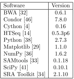
Table 1 lists the application software discussed above as well as the other installed and configured software needed to perform this experiment. This table does not include the platform components such as operating system packages or compilers necessary. All operating system packages were hosted on the deployment web server, as seen in Figure 6. The volume attached to the deployment web server stored a snapshot of operating system packages for the CentOS yum[10] repository as well as the Extra Packages for Enterprise Linux (EPEL) [39] yum repository. To control the experimental condi-tions on the operating system packages, the deployment web server in both clouds contained the same snapshot of operating system packages from repositories on the Internet.

Each application listed in Table 1 was also down-loaded from its original site on the Internet to the de-ployment web server in each individual cloud. All soft-ware installation and configuration scripts were created to accept configurable URLs for downloading software during deployment. This implementation allowed for controlling the version of application software.

The installation and configuration scripts were cre-ated and stored in the Chef server hosted in each cloud.

Software Version

BWA [32] 0.6.1

Condor [46] 7.8.0

Cython [4] 0.16

HTSeq [14] 0.5.3p6

Python [38] 2.7.3

Matplotlib [29] 1.1.0

NumPy [36] 1.6.2

SAMtools [33] 0.1.18

SciPy [41] 0.10.1

[image:6.612.372.502.50.188.2]

SRA Toolkit [34] 2.1.10

Table 1: Software Installed and Configured.

File Name

Homo sapiens.GRCh37.67.gtf.gz [1]

Homo sapiens.GRCh37.67.dna.chromosome.1.fa.gz [2] SRR001432.sra [3]

Table 2: Datasets

These software automation scripts provide the details of every configuration value, and installation command run to reproduce the installed environment. For ex-ample, to configure and install the numerical Python module NumPy [36], a Fortran compiler must be in-stalled. Determining the correct Fortran compiler and making sure the flags are set accordingly when compil-ing NumPy is but one example of how installation and configuration of the entire software stack can be chal-lenging toward the goal of experimental reproducibility. Through the use of software configuration management, this complexity is reduced anyone needing to reproduce the experiment.

The final piece of reproducing the experiment is hav-ing access to the original data. Table 2 lists the original files used to produce the charts. Similar to the software applications above, each of these files were downloaded to the deployment web server within each cloud from the original site on the Internet so that they could be de-ployed to the execute nodes when necessary. The sam-ple numbered SRR001432 from the Short Read Archive [8]. This sample is one of the H3K4me3 samples from [18].

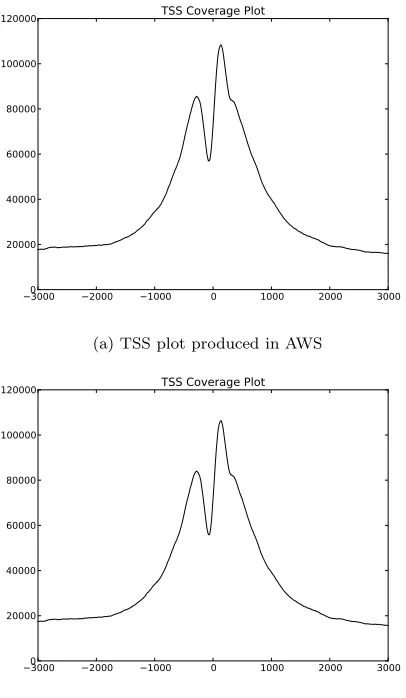
Table 3 outlines the high-level workflow executed to produce the charts in Figure 10. The applications were installed, and the workflow was executed in both the FutureGrid Eucalyptus and Amazon to produce the two TSS plots. Validating the data, we annotated one of the plots with a gray box from −200≤x≤50 because of

a “significant dip in the signal was observed between

(7)

1. Convert SRR001432.sra file to SRR001432.fastq

2. Gunzip Homo sapiens.GRCh37.67.gtf.gz→Homo sapiens.GRCh37.67.gtf

3. Extract chromosome 1 features from Homo sapiens.GRCh37.67.gtf→Homo sapiens.GRCh37.67 chrom1.gtf

4. Gunzip Homo sapiens.GRCh37.67.dna.chromosome.1.fa.gz→Homo sapiens.GRCh37.67.dna.chromosome.1.fa

5. Index Homo sapiens.GRCh37.67.dna.chromosome.1.fa

6. Align SRR001432.fastq to Homo sapiens.GRCh37.67.dna.chromosome.1.fa

7. Create SRR001432.sam

8. Create SRR001432.bam

9. Sort SRR001432.bam→SRR001432.sorted.bam

10. Index SRR001432.sorted.bam

11. Extract chromosome 1 from SRR001432.sorted.bam→SRR001432 head.bam

[image:7.612.330.533.323.477.2]

12. Use HTSeq[13] with Homo sapiens.GRCh37.67 chrom1.gtf and SRR001432 head.bam→TSS plot

Table 3: Steps to producing TSS plots

−30000 −2000 −1000 0 1000 2000 3000 20000

40000 60000 80000 100000

120000 TSS Coverage Plot

(a) TSS plot produced in AWS

−30000 −2000 −1000 0 1000 2000 3000 20000

40000 60000 80000 100000

[image:7.612.63.266.327.676.2]

(b) TSS plot produced in FutureGrid Eucalyptus

Figure 10: TSS plots produced in separate clouds

−30000 −2000 −1000 0 1000 2000 3000 20000

40000 60000 80000 100000

Figure 11: TSS plot annotated to confirm the significant dip in signal between−200≤x≤50.

5. CONCLUSIONS & FUTURE WORK

(8)

In the future we plan to extend this work in the following directions. First, we plan to expand further into the next generation sequencing pipelines to enable bioinformaticians to embed workflows into our frame-work so that these frame-workflows can be constructed in separate clouds. Additionally, we plan to extend this framework into educational uses to help lower barriers for people to use distributed environments. Incorporat-ing our framework in with other monitorIncorporat-ing tools like Ganglia[24] to provide researchers with the ability to monitor the experiment.

6. ACKNOWLEDGMENTS

This paper was developed with support from the Na-tional Science Foundation (NSF) under Grant No. 0910812 to Indiana University for “FutureGrid: An Experimen-tal, High–Performance Grid Test–bed.” Any opinions, findings, and conclusions or recommendations expressed in this material are those of the authors and do not nec-essarily reflect the views of the NSF.

7. REFERENCES

[1] ftp://ftp.ensembl.org/pub/release-67/gtf/homo sapiens/.

[2] ftp://ftp.ensembl.org/pub/release-67/fasta/homo sapiens/dna/.

[3]

ftp://ftp-trace.ncbi.nlm.nih.gov/sra/sra-instant/reads/ByRun/sra/SRR/SRR001/SRR001432/. [4] C-extensions for python. http://www.cython.org/. [5] Chef|Opscode. http://www.opscode.com/chef/. [6] Configuration management software| open source

configuration management CFEngine -distributed configuration management. http://cfengine.com.

[7] Hadoop.

[8] Home – SRA – NCBI.

http://www.ncbi.nlm.nih.gov/sra.

[9] Puppet labs: IT automation software for system administrators. http://www.puppetlabs.com/. [10] Yum. http://yum.baseurl.org/.

[11] A map of human genome variation from population-scale sequencing.Nature, 467(7319):1061–1073, 10 2010.

[12] Amazon Web Services LLC. Amazon EC2 instance types.

http://aws.amazon.com/ec2/instance-types/. [13] S. Anders. A detailed use case: TSS plots –

HTSeq v0.5.3p6 documentation. http://www-huber.embl.de/users/anders/HTSeq/doc/tss.html. [14] S. Anders. HTSeq: Analysing high-throughput

sequencing data with python – HTSeq v0.5.3p6 documentation.

http://www-huber.embl.de/users/anders/HTSeq/doc/index.html. [15] P. Anedda, S. Leo, S. Manca, M. Gaggero, and

G. Zanetti. Suspending, migrating and resuming

hpc virtual clusters.Future Generation Computer Systems, 26(8):1063 – 1072, 2010.

[16] M. Armbrust, A. Fox, R. Griffith, A. D. Joseph, R. H. Katz, A. Konwinski, G. Lee, D. A.

Patterson, A. Rabkin, I. Stoica, and M. Zaharia. Above the clouds: A berkeley view of cloud computing. Technical Report

UCB/EECS-2009-28, University of California at Berkeley, 2009.

[17] M. Baker. Next-generation sequencing: adjusting to data overload.Nat Meth, 7(7):495–499, 07 2010.

[18] A. Barski, S. Cuddapah, K. Cui, T.-Y. Roh, D. E. Schones, Z. Wang, G. Wei, I. Chepelev, and K. Zhao. High-resolution profiling of histone methylations in the human genome.Cell, 129(4):823–837, 05 2007.

[19] G. Bell, T. Hey, and A. Szalay. Beyond the data deluge.Science, 323(5919):1297–1298, 2009. [20] J. Bresnahan, T. Freeman, D. LaBissoniere, and

K. Keahey. Managing appliance launches in infrastructure clouds. InTeraGrid 2011, 2011. [21] F. Desprez, G. Fox, E. Jeannot, K. Keahey,

M. Kozuch, D. Margery, P. Neyron, L. Nussbaum, C. Perez, O. Richard, W. Smith, G. von

Laszewski, and J. V¨ockler. Supporting

experimental computer science. Technical Report 326, Argonne National Laboratory, 2012.

[22] K. Diethelm. The limits of reproducibility in numerical simulation.Computing in Science and Engineering, 14(1):64–72, 2012.

[23] J. Dudley and A. Butte. In silico research in the era of cloud computing.Nature Biotechnology, pages 1181–1185, 2010.

[24] D. Federico, M. J. K. Sacerdoti, M. L. Massie, and D. E. Culler. Wide area cluster monitoring with ganglia. InIEEE International Conference on Cluster Computing, 2003.

[25] I. Foster, T. Freeman, K. Keahey, D. Scheftner, B. Sotomayor, and X. Zhang. Virtual clusters for grid communities. InProc. of the 6h IEEE Int. Symp. on Cluster Computing and the Grid, pages 513–520, 2006.

[26] R. Goldberg. Survey of virtual machine research. InIEEE Computer, pages 34–45, 1974.

[27] T. Hey, S. Tansley, and K. Tolle. Jim gray on escience: A transformed scientific method.

Microsoft Research, 2009.

[28] B. Howe. Virtual appliances, cloud computing, and reproducible research.Computing in Science & Engineering, 99(PrePrints), 2012.

[29] J. Hunter, D. Dale, and M. Droettboom. matplotlib. http://matplotlib.sourceforge.net/. [30] H. Kim and M. Parashar. CometCloud: an

(9)

Principles and Paradigms, chapter 10. Wiley, 2011.

[31] S. Leo, P. Anedda, M. Gaggero, and G. Zanetti. Using virtual clusters to decouple computation and data management in high throughput analysis applications. InProc. of the Euromicro Conference on Parallel, Distributed, and

Network-Based Processing, pages 411–415, 2010. [32] H. Li and R. Durbin. Fast and accurate short read

alignment with burrows-wheeler transform.

Bioinformatics, 2009.

[33] H. Li, B. Handsaker, A. Wysoker, T. Fennell, J. Ruan, N. Homer, G. Marth, G. Abecasis, R. Durbin, and et. al. The sequence

alignment/map (sam) format and samtools.

Bioinformatics, 2009.

[34] National Center for Biotechnology Information. Sra toolkit.

http://www.ncbi.nlm.nih.gov/Traces/sra/. [35] NIH. 1000 genomes project data available on

amazon cloud. Press Release, March 2012.

http://www.nih.gov/news/health/mar2012/nhgri-29.htm.

[36] Numpy developers. Scientific computing tools for python – numpy. http://numpy.scipy.org/. [37] D. Nurmi, R. Wolski, C. Grzegorczyk,

G. Obertelli, S. Soman, L. Youseff, and D. Zagorodnov. The eucalyptus open-source cloud-computing system. InProc. of the 2009 9th

IEEE/ACM Int. Symp. on Cluster Computing and the Grid, pages 124–131, 2009.

[38] Python Software Foundation. Python programming language – official website. http://www.python.org/.

[39] Red Hat. EPEL - FedoraProject. http://fedoraproject.org/wiki/EPEL.

[40] M. C. Schatz, B. Langmead, and S. L. Salzberg. Cloud computing and the dna data race.Nature Biotechnology, 28(7):691—693, 2010.

[41] Scipy Community. Scipy. http://www.scipy.org/. [42] S. Staff. Challenges and opportunities.Science,

331(6018):692–693, 2011.

[43] L. D. Stein. The case for cloud computing in genome informatics.Genome Biology, 2010. [44] T. Tannenbaum, D. Wright, K. Miller, and

M. Livny. Condor – a distributed job scheduler. In

Beowulf Cluster Computing with Linux. MIT Press, 2001.

[45] Team. Algorithms for the grid: Inria research proposal.

http://www.loria.fr/equipes/algorille/algorille2.pdf. [46] The Condor Team. Condor project homepage.

http://research.cs.wisc.edu/condor/.

Using Cloud Computing for Scalable, Reproducible Experimentation