Standard Statistical and Graph based Automatic Keyword Extraction

International Journal of Innovative Technology and Exploring Engineering (IJITEE) ISSN: 2278-3075, Volume-9 Issue-2, December 2019

Standard Statistical and Graph based Automatic

Keyword Extraction

G. Kannan, R.Nagarajan

Abstract: Automatic extraction of terms from a document is essential in the current digital era to summarize the documents. For instance, instead of go through the full documents, some of the author's keywords partially explain the discussions of the documents. However, the author's keywords are not sufficient to identify the whole concept of the document. Hence the requirement of automatic term extraction methods is necessary. The major categories of automatic extraction approaches falls mainly on some techniques such as Natural Language Processing, Statistical approaches, Graph Based approaches, Natural Inspired algorithmic approaches, etc. Even though there are numerous approaches available the exact automatic keyword extraction is a major challenge in areas, that reveals around documents. In this paper, a comparative analysis of Keyword extraction between standard Statistical approaches and Graph based approaches has been conducted. In standard statistical approaches, the terms are extracted on the basis of physical counts and in the Graph based approach, the documents are automatically constructed as graphs by applying centrality measures during the keyword extraction process. The results of both approaches were compared and analyzed.

Keywords: Statistical methods ,Graph based methods, Keyword Extraction, Centrality measures.

I. INTRODUCTION

Keywords are the smallest units that can summarize the concept of a documentand are often used to pinpoint the most relevant information in a text. Keywords are used for various purposes, like retrieving documents during a web search or summarizing the documents for indexing. Keywords in a document provide important information about the content of the document. They can help the users search through information more efficiently or decide whether to read a document or not to read the document. They can also be used for a variety of language processing tasks such as text categorization and information retrieval. Assigning the keywords manually is impossible because, over the past one decade, a great evolution of computer technology has provided more reasonable and high configuration systems. The bursty data is increasing every day, so we need to maintain and analyze the data for effective use or processing. Data can be available in the form of image, spatial form, text; mostly text data is represented in many ways like text, graphs, predicates, etc. keyword extraction play big roll in text mining process because, in the newspaper, social media are used for posting and messaging and all the information of company contained in the form of text.

Revised Manuscript Received on December 05, 2019.

G. Kannan, Assistant Professor, Govt. Arts and Science College, Manalmedu, India.

Dr. R.Nagarajan, Assistant Professor, Division of Computer and Information Science, Annamalai University, Annamalainagar, India.

Automatic keyword extraction is the process of selecting words and phrases from the text document that can best describe the concept of the document without any human intervention. The goal of automatic keyword extraction is the power and speed of current computation abilities to solve the problems in access and recovery, and the problems related to information organization without added human interactions. Organize the long-lasting growth of vibrant unstructured documents is the major challenge and handling such unorganized documents causes more expensive. The clustering of such dynamic documents helps us to reduce the cost. Document clustering by analyzing the keywords of the documents is one of the best methods to organize the unstructured dynamic documents.

II. LITERATURE REVIEW

In this section, we evaluate the prior works on keyword extraction methods and assert how unique these methods are discussed. Floarin Boudin presented the centrality measures, comparison for extraction of keywords in Graph based approaches, the closeness centrality obtain the optimum results on short – documents [1]. The new unsupervised technique for spontaneously sentence extraction using a Graph based Ranking algorithm focused on [2]. The authors have projected the new Graph based keyword extraction algorithm, the terms as vertices, the relationship between the terms as arcs, and the projected algorithm which gives more accurate result [3]. Sonawane et al. [4] presented a centrality measure and compare the five centrality measures (Degree centrality, Betweeness Centrality, Closeness Centrality, Eigenvector centrality, and Text rank). The authors deal with the document BOW, and finally, the authors say the graph based text representation is the best way and the result is better than the traditional model [5]. A new graph based approach for text categorization, the authors conclude the graph based methods are efficient then statistical t –methods projected [6]. Alwan M Ubaidillah et al. proposed and conform two graph based methods, cross-lingual key term extraction to be used in extractive content summarization in [7]. The grow up continuous digital news, modeling digital news data stored in the database. It will be easy to understand and be able to take the information immediately, of the MCL graph clustering algorithm is used [8]. The author focused on the frequency-based methods, weight to the word in the graph and TF and the TF-IDF [9]. Florian Boudin has dealt with keyterm extraction which to identify the main topics of the documents by topic rank, candidates keyphrases which are clustered into topics, and the topic rank significantly out performs the state-of-art methods in [10]. In [11] discussed problems for keyword and key phrase extraction

rank algorithm. The authors have presented a survey for text summarization techniques, which deals with the necessity of text summarization, we review the various processes of text summarization and express the viability and deficiencies of the different techniques [12]. In [13] introduced extract the keyword for web site clustering, we propose a clustering method automatic keyword extraction of the keywords of a web page. The graph based representation, for plain text, using context and keyword extraction in [14]. Santhosh Kumar et al. introduced an investigation for extracting the key term without human intervention in text summarization, talk about the various tactic used for key term extraction and text summarization [15]. In [16], presented the facet extraction techniques for the subgraph to reduce the burden for search data in graphs. In [17 - 21] presented frequent subgraph the mining techniques to derive the coherent subgraphs. In [22] presented a review for keyword extraction techniques, discussed feature selection metrics.

A. Keyword Extraction Methods

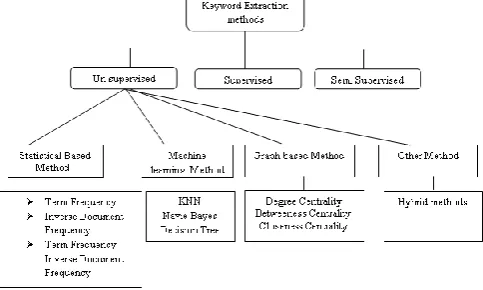
Keyword extraction methods, mainly, are divided into Supervised and Unsupervised approaches. In the Supervised approach, training dataset is maintained. In the Unsupervised approach , the approach doesn‟t need training data. In this paper, standard statistical methods and Graph based methods (Unsupervised methods) of keyword extraction have been analyzed.

B. Simple Statistics

These approaches are simple and don't require training information. The keyword statistics can be utilized to formulate the key terms:- n gram measurements, word recurrence, TFIDF, word co-event are some of the examples.

C. Linguistics

This approach utilizes the dialectal properties of the words, sentences and documents. A portion of the etymology includes the syntactic, lexical, etc. For NLP issues this technique can be applied.

D. Machine Learning

This approach depends upon the processed information to extract the keyword. It requires manual explanations for the learning dataset which is extremely monotonous and incompatible. The SVM (support vector machine), and the Naïve Bayes are some of the examples.

E. Graph Based

These approaches are simple mathematical models, which enable the exploration of the relationships and make the structural information meaningful. The graph is a discrete data structure consisting of nodes and edges ={V, E}

Vertices also referred to as node, and Edges are the lines or arcs, which connect the nodes in the graph. The document is modeled as graph the terms (words) are represented by vertices(nodes) and their relationship is represented as edges(link). In the Graph based method, the graph describes the meaning of the document visually. Initially, the document is converted into graph,

and the keywords of the document are found. Graph nodes represent only meaningful words of the documents

F. Other approaches

These approaches are integrated approaches of standard approaches such as Statistical approaches, Linguistics approaches, Machine learning approaches, and Graph based approaches.

Fig. 1. Different Keyword Extraction methods

III.METHODOLOGY

This section focuses attention on the various existing keyword extraction approaches found in the standard statistical methods and Graph based methods.

A. Simple Statistics Method

Generally, statistics methods take in to accounts the occurrences of the term. It is very simple and the results are visually satisfying . It identifies the important terms, based on the number of appearances in the documents. The most frequently used keyword extraction of the statistical methods is Term Frequency(TF) and Inverse Document Frequency(IDF).

 TF:(Term Frequency): The TF is the straight forward statistical method which finds out the frequency of term used in the documents. It merely takes the more frequent term by calculating with occurrences. If the document size is a high number of the key term may be derived otherwise it extracts very few. The TF can be calculated by using the following formula.

corpus in the Words Total

count(w) Document

) (w 

TF (1)

 IDF:(Inverse Document Frequency):The IDF always comes along with TF, it helps to identify the more common terms of the documents, which occur more frequently in the documents.

While calculating the term incidence, each term is considered equally important and given chance to contribute in vector representation, but the assured words which are so general from corner to corner in the documents that they may donate very little in deciding the meaning of it.

International Journal of Innovative Technology and Exploring Engineering (IJITEE) ISSN: 2278-3075, Volume-9 Issue-2, December 2019

The IDF can be calculated by using the following formula.

word(w) containing

documents of

Number

documents) of

Number log(Total

) (w 

IDF (2)

 TF-IDF: (Term Frequency – Inverse Document Frequency):The TF-IDF vector portrayal gives transcending incentive for a given term if it happens frequently in that specific record or once in a while anywhere else. In the event the term happen in every of the reports, the IDF figured would be TF-IDF giving the result of term recurrence and backward record recurrence. The more important a term used in the document, would get a higher TF-IDF score and vice versa

The TF-IDF can be calculated by using following formula: TF-IDF(w) = tf(w)*idf(w) (3)

B. Graph Based Method

Usually, Graphs are mathematical model, generally graphs as represented as G= {V,E}

V- Vertices E- Edges

In Graph based keyword extraction methods, the important terms are represented as vertices, the association between the vertices are linked, the links represented as Edges. Centrality measures are mainly used to find the key terms from the Graph in the Graph based keyword extraction methods

 Degree Centrality: The Degree centrality, it takes in to account the number of the adjoined nodes. If the network is directed, two types of the measures, in-degree : computes the number of inward links or the number of predecessor nodes; out-degree: computes the number of departing links or the number of successor nodes.

As per degree centrality concerns, a node is important if it has many adjoined nodes.

The degree centrality of a node vi is calculated as:

-1

|

V

|

|

N(Vi)

|

=

CD(Vi)

where,

 CD(Vi) is the degree the centrality of node Vi  V is the set of nodes

 N(Vi) is the set of nodes connected to the node Vi 

 Closeness Centrality: This centrality is depicts as the corresponding of the aggregate of separations of all nodes to certain nodes, i.e., contrary of farness. The closeness centrality of the node Vi is given in the following equation.

In a linked graph, the closeness centrality of a node is a calculated centrality in a graph, which is calculated as the sum of the space of the shortest paths between the node and all other nodes in the graph. Thus, the more vital a node is, the nearer it is to all other nodes.

Vj)

,

dist(Vi

Vi€V

-1)

|

V

(|

=

)

(V

C

where

 The CC(Vi) is closeness centrality of the node Vi  The V is the set of nodes (words) in the graph G  The dist(Vi,Vj) is the shortest distance between nodes

Vi and Vj

 Betweeness Centrality: Betweeness Centrality is a process of centrality in a graph depending on the least way. For each couple of vertices in a connected graph, there exists, at any, rate one most brief way between the vertices to such an extent that either the quantity of edges that the way goes through (for unweighted charts) or the whole of the loads of the edges (for weighted charts) are limited. In the betweeness centrality, for every vertex, the quantity of these most limited ways go through the vertex.

(6) Where

The CB (Vi) is Betweeness Centrality of node Vi

The σ(Vj, Vk) is the number of shortest paths from nodeVjto

nodeVk

The σ(Vj, Vk| Vi) is the number of those path that pass

through the node Vi

IV. EXPERIMENTAL RESULT

To compare the standard statistical and graph based keyword extraction methods, 14 documents have been taken, which are shown in the following Table -1.

Table–I: Sample Documents

Document Id

Document

D1 In imaging science, image processing is processing of images using mathematical operations by using any form of signal processing.

D2 In Image Processing, the input is an image, a series of images, or a video, such as a photograph or video frame; the output of image processing may be either an image or a set of characteristics or parameters related to the image.

D3 Most image-processing techniques involve treating the image as a two-dimensional signal and applying the standard signal-processing techniques to it.

D4 Images are also processed as three-dimensional signals where the third-dimension being time or the z-axis. D5 Image processing usually refers to digital image

processing, but the optical and analog image processing also are possible.

D6 This article is about general techniques that apply to all of them. The acquisition of images (producing the input image in the first place) is referred to as imaging. Closely related to image processing are computer graphics and computer vision.

D7 In computer graphics, images are manually made from physical models of objects, environments, and lighting, instead of being acquired (via imaging devices such as cameras) from natural scenes, as in most animated movies.

D8 Computer vision, on the other hand, is often considered high-level image processing out of which a machine/computer/software intends to decipher the physical contents of an image or a sequence of images (e.g., videos or 3D full-body magnetic resonance scans). D9 Computer graphics are pictures and movies created using computers, such as CGI - usually referring to image data created by a computer specifically with help from specialized graphical hardware and software. D10 It is a vast and recent area in computer science. The

phrase was coined by computer graphics researchers Verne Hudson and William Fetter of Boeing in 1960. D11 Another name for the field is computer-generated

D12 The overall methodology depends heavily on the underlying sciences of geometry, optics, and physics. Computer graphics is responsible for displaying art and image data effectively and beautifully to the user, and processing image data received from the physical world. D13 The interaction and understanding of computers and

interpretation of data has been made easier because of computer graphics.

D14 Computer graphic development has had a significant impact on many types of media and has revolutionized animation, movies, advertising, video games, and graphic design generally.

In table -1, the first column represents the document ID, the second column represents documents. At this stage, the documents contain all the terms. In the analysis, the standard preprocessing techniques used help reduce the size of the document. The standard preprocessing techniques include Tokenization, Stop word Removal and Stemming. After applying the preprocessing techniques, the term „in‟, „is‟, ‟of‟,‟ using‟, ‟by‟, ‟any‟, ‟form‟, and ‟of‟ are removed with the help of stop word removal technique. Similarly, the terms „imaging‟, and „images‟ denote the root word „image‟. With the help of stemming process, because this technique identifies the root word, all the documents are automatically preprocessed. Finally, the noise removed terms are maintained in the following table-2 for the further process.

Fig. 2. Proposed Graph based Keyword Extraction method

Table-II: Extracted Terms in the Documents

Document Id

Extracted Terms

D1 „IMAGE‟ , „SCIENCE‟, „PROCESSING‟, „SIGNAL‟, „MATHEMATICAL‟, „OPERATION‟

D2 „IMAGE‟, „SERIES‟, „PROCESSING‟, „VIDEO‟, „PHOTOGRAPH‟ ,„FRAME‟

D3 „IMAGE‟, „PROCESSING‟, „TELEVISION‟, „TWO-DIMENSION‟, „SIGNAL‟

D4 „IMAGE‟, „PROCESSING‟, „THREE-DIMENSION‟, „Z-AXIS‟ ,„SIGNAL‟

D5 „IMAGE‟, „PROCESSING‟, „DIGITAL‟, „ANALOG‟, „OPTICAL‟

D6 „ACQUISITION‟, „IMAGE‟, „PROCESSING‟, „COMPUTER‟ ,„VISION‟, ‟GRAPHICS‟

D7 „COMPUTER‟,„GRAPHICS‟,„IMAGE‟,„ACQUIRED‟,„LI GHT‟,„ENVIRONMENT‟ , „PHYSICAL‟ ,„MODEL‟, „OBJECT‟, „ANIMATION‟, „MOVIE‟

D8 „COMPUTER‟, „VISION‟, „IMAGE‟, „PROCESSING‟ D9 „COMPUTER‟ ,„GRAPHICS‟, „PICTURE‟, „MOVIE‟,

„IMAGE‟, „DATA‟, „SOFTWARE‟ D10 „COMPUTER‟ „SCIENCE‟ „GRAPHICS‟

D11 „COMPUTER‟ „VIDEO‟ „IMAGE‟ „GRAPHICS‟ „SPRITE‟ „VECTOR‟

D12 „SCIENCE‟ „OPTICS‟ „PHYSICS‟ „GEOMETRY‟ „COMPUTER‟ „GRAPHICS‟ „IMAGE‟ „DATA‟ „PROCESSING‟

D13 „COMPUTER‟ „DATA‟ „GRAPHICS‟

D14 „COMPUTER‟ „GRAPHICS‟ „ANIMATION‟ „MOVIE‟ „ADVERTISEMENT‟ „VIDEO GRAPH‟

A. Graph Construction

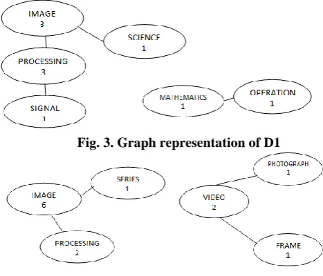
At this stage, the undirected word graph is built for each document in a corpus, in which the documents are represented as graph. In each document, the terms are referred as nodes; and the repetitive associations, between the words of the documents, are referred as the edges. By using syntactic filters, the vertices of graph are filtered; the repetitive count of the words determines the arcs. By using the above said strategy, the extracted terms, from the table-2, were taken to built the graphs, which best portray the document‟s conception. During the graph construction, the association between the nodes is drawn as the edges depending on their position in the document. For instance, the following graph-1 represents document id 1. From the following graph, it is observed that the nodes image, processing, science and signals form a separate connected component of the graph and the nodes, mathematics and operation form a separate connected component of the graph. This shows the document id 1, which deals with two slightly different concepts.

Fig. 3. Graph representation of D1

Fig. 4. Graph representation of D2 The following graph 2 - represents the graph form of document id 2. From the above graph, it is observed that the nodes image, processing, and series form a separate connected component of a graph and the nodes videos, photograph and frame form a separate connected component of the graph. This shows the document id 2, which describe the two different concepts (indirectly related). Likewise, the remaining documents have been processed. Similarly all the 14 documents were converted into graphs.

B. B. Word Determination

When the word graph is built, the significant word determination step is pursued,

International Journal of Innovative Technology and Exploring Engineering (IJITEE) ISSN: 2278-3075, Volume-9 Issue-2, December 2019

out the position of every node in a graph. In graph hypothesis, centrality measures allude the markers which recognize the most significant vertices inside a graph and

that approach is utilized for the errand of positioning the nodes.

Table-IV: Betweeness Centrality

Term D1 D2 D3 D4 D5 D6 D7 D8 D9 D10 D11 D12 D13 D14 CB(Vi)

Image 2.0000 1.0000 1.0000 0.0000 5.0000 4.0000 24.0000 8.0000 6.0000 0.0000 0.0000 4.0000 0.0000 0.0000 3.9286 Computer 0.0000 0.0000 0.0000 0.0000 0.0000 6.0000 7.0000 0.0000 10.0000 1.0000 6.0000 0.0000 1.0000 0.0000 2.2143 Graphics 0.0000 0.0000 0.0000 0.0000 0.0000 0.0000 0.0000 0.0000 10.0000 0.0000 6.0000 3.0000 0.0000 10.0000 2.0714 Processing 2.0000 0.0000 3.5000 3.0000 0.0000 6.0000 0.0000 0.0000 0.0000 0.0000 0.0000 0.0000 0.0000 0.0000 1.0357 Physical 0.0000 0.0000 0.0000 0.0000 0.0000 0.0000 12.0000 0.0000 0.0000 0.0000 0.0000 0.0000 0.0000 0.0000 0.8571 3d 0.0000 0.0000 0.0000 0.0000 0.0000 0.0000 0.0000 8.0000 0.0000 0.0000 0.0000 0.0000 0.0000 0.0000 0.5714 Model 0.0000 0.0000 0.0000 0.0000 0.0000 0.0000 7.0000 0.0000 0.0000 0.0000 0.0000 0.0000 0.0000 0.0000 0.5000 Picture 0.0000 0.0000 0.0000 0.0000 0.0000 0.0000 0.0000 0.0000 6.0000 0.0000 0.0000 0.0000 0.0000 0.0000 0.4286

3-dimension 0.0000 0.0000 0.0000 5.0000 0.0000 0.0000 0.0000 0.0000 0.0000 0.0000 0.0000 0.0000 0.0000 0.0000 0.3571 Vision 0.0000 0.0000 0.0000 0.0000 0.0000 0.0000 0.0000 5.0000 0.0000 0.0000 0.0000 0.0000 0.0000 0.0000 0.3571

Table-V: Closeness Centrality

Term D1 D2 D3 D4 D5 D6 D7 D8 D9 D10 D11 D12 D13 D14 CC(Vi)

Image 0.7500 1.0000 0.6600 0.4444 0.8000 0.5000 0.6666 0.6000 0.4666 0.0000 0.4545 0.8000 0.0000 0.0000 0.5102

Computer 0.0000 0.0000 0.0000 0.0000 0.0000 0.6250 0.4705 0.3333 0.6363 1.0000 0.7142 0.4444 1.0000 0.5555 0.4128

Graphics 0.0000 0.0000 0.0000 0.0000 0.0000 0.4166 0.3333 0.0000 0.5384 0.6666 0.7142 0.6666 0.6666 1.0000 0.3573

Processing 0.7500 0.6600 0.8000 0.6666 0.5000 0.6250 0.0000 0.4000 0.0000 0.0000 0.0000 0.5714 0.0000 0.0000 0.3552

Science 0.5000 0.6600 0.0000 0.0000 0.0000 0.0000 0.0000 0.0000 0.0000 0.6666 0.0000 1.0000 0.0000 0.0000 0.2019

Signal 0.5000 0.0000 0.6600 0.6666 0.0000 0.0000 0.0000 0.0000 0.0000 0.0000 0.0000 0.0000 0.0000 0.0000 0.1305

Data 0.0000 0.0000 0.0000 0.0000 0.0000 0.0000 0.0000 0.0000 0.3333 0.0000 0.0000 0.5714 0.6666 0.0000 0.1122

Video 0.0000 1.0000 0.0000 0.0000 0.0000 0.0000 0.0000 0.0000 0.0000 0.0000 0.0000 0.0000 0.0000 0.5555 0.1111

Vision 0.0000 0.0000 0.0000 0.0000 0.0000 0.4166 0.0000 0.4615 0.0000 0.0000 0.4545 0.0000 0.0000 0.0000 0.0952 In the area of keyword extraction, different centrality

measures are utilized for the errand of positioning the words in documents.

C. Centrality Measures

After the conversion of documents into graphs, to extract the important terms from the graphs, three centrality measures namely Degree Centrality, Betweeness Centrality and Closeness Centrality measures had been applied to the graphs. The resulted numeric values were placed in Table 3, Table 4 and Table 5 respectively.

 Degree Centrality: Initially, when this method is applied for all the documents, the result of Degree centrality method with 40 keywords are identified based on the thrash hold value (automatically assigned based on the size of the document), which will minimize the size of the keyword. Finally top-ranked keywords are taken are shown in the Table 3.

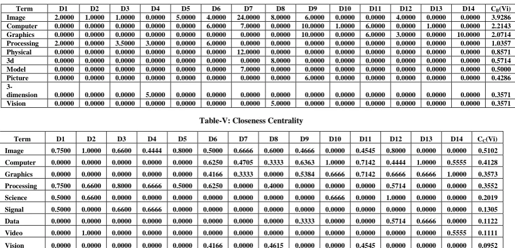
 Betweeness Centrality: While the Betweeness centrality method is applied for all the 14 documents, result of the Betweeness centrality method 16 keywords are identified based on the thrash hold value, it will produce top-ranked keywords are shown in the Table 4.

 Closeness Centrality: Finally, when the Closeness centrality method is applied for the same documents, the result of the Closeness centrality method with 40 keywords

are identified, based on the thrash hold value the top-ranked keywords are identified in the Table 5.

In the graph based methods Degree centrality, Betweeness centrality and Closeness centrality results are analyzed and the first four top-ranked keywords are identified: which are, „image‟, „computer‟, „graphics‟, „processing‟. The result is the same for all the three methods. The remaining keywords are found with same degree of centrality and Closeness centrality, and little difference in Betweeness centrality, since the properties of the Degree centrality and Closeness centrality are nearly same. The node appearing in the graph gets some weight, but in Betweeness centrality it is different from above methods; in the Betweeness centrality, the method weight of the node is calculated only when the particular node has more number of shortest paths pass via the node. In this nature, the Degree centrality and the Closeness centrality is found more similar than the Betweeness centrality.

D. Statistical methods

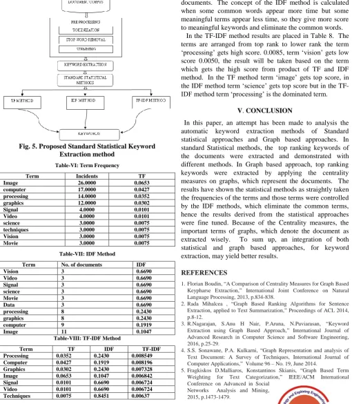
Standard statistical methods, TF, IDF and TF-IDF, were applied on raw terms extracted from documents. The results of TF method is shown in the following table 6, the result of IDF method is shown in

Table 7 and result of TF-IDF method is shown in Table 8. Table-III: Degree Centrality

Term D1 D2 D3 D4 D5 D6 D7 D8 D9 D10 D11 D12 D13 D14 CD(Vi)

 Term Frequency: The top ranking terms identified by TF method are „image‟, ‟computer‟, ‟processing‟, ‟graphics‟, ‟signal‟, ‟video‟, „science‟, ‟technique‟, ‟vision‟, ‟movie‟.

 Inverse Document Frequency: The top ranking terms identified by IDF method are, „signal‟, „video‟, „science‟, ‟processing‟, „vision‟, „movie‟, „data‟, „processing‟, „graphics‟, „computer‟, „image‟ were identified.

 Term Frequency-Inverse Document Frequency: The top ranking terms where identified by TF-IDF method are, was „processing‟ , „computer‟, „image‟, „graphics‟, „ signal‟, „video‟, „science‟.

Fig. 5. Proposed Standard Statistical Keyword Extraction method

Table-VI: Term Frequency

Term Incidents TF Image 26.0000 0.0653 computer 17.0000 0.0427 processing 14.0000 0.0352 graphics 12.0000 0.0302 Signal 4.0000 0.0101 Video 4.0000 0.0101 science 3.0000 0.0075 techniques 3.0000 0.0075 Vision 3.0000 0.0075 Movie 3.0000 0.0075

Table-VII: IDF Method

Term No. of documents IDF Vision 3 0.6690 Video 3 0.6690 Signal 3 0.6690 science 3 0.6690 Movie 3 0.6690 Data 3 0.6690 processing 8 0.2430 graphics 8 0.2430 computer 9 0.1919 Image 11 0.1047

Table-VIII: TF-IDF Method

Term TF IDF TF-IDF Processing 0.0352 0.2430 0.008549 Computer 0.0427 0.1919 0.008196 Graphics 0.0302 0.2430 0.007328 Image 0.0653 0.1047 0.006842 Signal 0.0101 0.6690 0.006724 Video 0.0101 0.6690 0.006724 Techniques 0.0075 0.8451 0.00637

Acquisition 0.0050 1.1461 0.005759 Science 0.0075 0.6690 0.005043 Vision 0.0075 0.6690 0.005043

From the table 6, which shows the top ranked terms derived from TF method, „image‟ occurred 26 times ,gets the score 0.0653, so it captured the first position, similarly, the remaining terms are arranged from top to bottom based on the score. The term „movie‟ occurred 3 times, gets the score 0.0075only so it is placed at the last place. From the table7, shows the top ranked terms derived from IDF method, „vision‟, gets the score 0.6690 but it appears only in 3 documents out of 14 documents. The term „image‟ gets the score 0.1047 but it appears in 11 documents out of 14 documents. The concept of the IDF method is calculated when some common words appear more time but some meaningful terms appear less time, so they give more score to meaningful keywords and eliminate the common words. In the TF-IDF method results are placed in Table 8. The terms are arranged from top rank to lower rank the term „processing‟ gets high score. 0.0085, term „vision‟ gets low score 0.0050, the result will be taken based on the term which gets the high score from product of TF and IDF method. In the TF method term „image‟ gets top score, in the IDF method term „science‟ gets top score but in the TF-IDF method term „processing‟ is the dominated term.

V. CONCLUSION

In this paper, an attempt has been made to analysis the automatic keyword extraction methods of Standard statistical approaches and Graph based approaches. In standard Statistical methods, the top ranking keywords of the documents were extracted and demonstrated with different methods. In Graph based approach, top ranking keywords were extracted by applying the centrality measures on graphs, which represent the documents. The results have shown the statistical methods as straightly taken the frequencies of the terms and those terms were controlled by the IDF methods, which eliminate the common terms, hence the results derived from the statistical approaches were fine tuned. Because of the Centrality measures, the important terms of graphs, which denote the document as extracted wisely. To sum up, an integration of both statistical and graph based approaches, for keyword extraction, may yield better results.

REFERENCES

1.Florian Boudin, “A Comparison of Centrality Measures for Graph Based

Keypharse Extraction,” International Joint Conference on Natural Language Processing, 2013, p.834-838.

2.Rada Mihalcea , “Graph Based Ranking Algorithms for Sentence

Extraction, applied to Text Summarization,” Proceedings of ACL 2014, p.8-12.

3.R.Nagarajan, S.Anu H Nair, P.Aruna, N.Puviarasan, “Keyword

Extraction using Graph Based Approach,” International Journal of Advanced Research in Computer Science and Software Engineering, 2016, p.25-29.

4.S.S. Sonawane, P.A. Kulkarni, “Graph Representation and analysis of

Text Document: A Survey of Techniques, International Journal of Computer Applications,” Volume 96 – No. 19, June 2014.

5.Fragkiskos D.Malliaros, Konstantinos Skianis, “Graph Based Term

Weighting for Text Categorization,” IEEE/ACM International Conference on Advanced in Social

International Journal of Innovative Technology and Exploring Engineering (IJITEE) ISSN: 2278-3075, Volume-9 Issue-2, December 2019

6.Marina Litvak, Mark Last,Graph Based Keyword Extraction for

Single-Document Summarization, Coling,2008, Proceedings of the workshop Multilingual Information Extraction and Summarizartion, p.17-24.

7.Alwan M Ubaidillah Al-Fath, Kemas Rahmat Saleh W., M.Eng, Siti

Sa‟adah,M.T., “Implementation of MCL Algorithm in Clustering Digital News with Graph Representation,” IEEE, 2016.

8.F.Sebastiani, “Machine Learning in automated text categorization,”

ACM Computer surv., Vol. 34, no.1, p.1-47, 2002.

9.Adrien Bougouin, Florian Boudin, Beatrice Daille, “Topic Rank: Graph

Based Topic Ranking for Keypharse Extraction,” International Joint Conference on Natural Language Processing, 2013, p.543-551.

10. Florian Boudin, “A Comparison of Centrality Measures for Graph

Based Keypharse Extraction,” International Joint Conference on Natural Language Processing, 2013,p.834-838.

11. Shibamouli Lahiri, Sagnik Ray Choudhury, Cornelia Caragea,

“Keyword and Keypharse Extraction Using Centrality Measures on Collocation Networks,” arXiv:1401.6571vl [cs.CL], 2014.

12. Mehdi Allahyari, Seyedamin Pouriyeh, Mehdi, Assefi, Saeid Safaei,

Elizabeth D. Trippe, Juan B. Gutierres, Krys Kochut, Text Summarization Techniques: A Brief Survey, arXiv, USA, 2017.

13. Paolo Tonelia, Filippo Ricca, Emanuele Pianta and Christian Girardi,

“Using Keyword Extraction for website Clustering,” Proceedings of the Fifth IEEE International Workshop on Web Site Evolution (WSE‟03), 2003.

14. C.Abi Chahine, N. Chaignaud, JPh Kotowicz, JP Pecuchet, “Context

and Keyword Extraction in Plain Text Using a Graph Representation,” IEEE, 2008.

15. Santhosh Kumar Bharathi, Korra sathya Babu, Sanjay Kumar Jena,

“Automatic Keyword Extraction for Text Summarization: A Survey,” NIT, Rurkela, Odisha,2017.

16. Takahiro Komamizu, Toshiyuki Amagasa, Hiroyuki Kitagawa,

“Frequent-Pattern based Facet Extraction from Graph Data,” International Conference on Network-Based Information Systems, 2014, p.318 – 323.

17. L.B. Holder, D.J. Cook, S. Djoko, “Substructure Discovery in the

SUBDUE system,” in proc. KDD Workshop, 1994, pp.111-122.

18. S. Ghazizadeh, S.S. Chawathe, “SUES: Structure Extraction Using

Summaries,” in Proc. Discovery Science, ser. Lecture Notes in Computer Science, Vol.2534, Springer, 2002, pp.71-85.

19. M. Fiedler, C. Borgelt, “Support Computation for Mining Frequent

Subgraphs in a Single Graph,” in MLG,2007.

20. Ananth C, Karthikeyan M and Mohananthini N., “Literature Survey on

multiple image watermarking Techniques with Genetic Algorithm”, Advances in Natural and Applied Sciences. 11(6); 2017, pp. 237-257.

21. N. Mohananthini, G. Yamuna, C Ananth and M Karthikeyan,

“Literature Review on Multiple Watermarking for Images using Optimization Techniques”, International Journal of Advanced Research in Electrical, Electronics and Instrumentation Engineering, Vol. 6, Issue 6, pp. 4455-4463, 2017.

22. Sifatullah Siddiqi, Aditi Sharan, “ Keyword and Keypharse Extraction

Techniques: A Literature Review, “ International Journal of Computer Applications, vol. 109-No.2, 2015.

AUTHORS PROFILE

Kannan G received his Bachelor Degree from Annamalai University, Tamilnadu, India in 2001. He received his Master Degree from Annamalai University, Tamilnadu, India in 2004. Currently, he is working as Assistant Professor in the Department of Computer Science, Govt. Arts and Science College, Manalmedu, Tamilnadu, India. His current research area is data mining.