Hierarchically Clustered Adaptive Quantization
CMAC and Its Learning Convergence
S. D. Teddy, E. M.-K. Lai
, Senior Member, IEEE
, and C. Quek
Abstract—The cerebellar model articulation controller (CMAC) neural network (NN) is a well-established computational model of the human cerebellum. Nevertheless, there are two major drawbacks associated with the uniform quantization scheme of the CMAC network. They are the following: 1) a constant output resolution associated with the entire input space and 2) the gen-eralization-accuracy dilemma. Moreover, the size of the CMAC network is an exponential function of the number of inputs. Depending on the characteristics of the training data, only a small percentage of the entire set of CMAC memory cells is utilized. Therefore, the efficient utilization of the CMAC memory is a crucial issue. One approach is to quantize the input space nonuni-formly. For existing nonuniformly quantized CMAC systems, there is a tradeoff between memory efficiency and computational complexity. Inspired by the underlying organizational mechanism of the human brain, this paper presents a novel CMAC architec-ture named hierarchically clustered adaptive quantization CMAC (HCAQ-CMAC). HCAQ-CMAC employs hierarchical clustering for the nonuniform quantization of the input space to identify significant input segments and subsequently allocating more memory cells to these regions. The stability of the HCAQ-CMAC network is theoretically guaranteed by the proof of its learning convergence. The performance of the proposed network is subse-quently benchmarked against the original CMAC network, as well as two other existing CMAC variants on two real-life applications, namely, automated control of car maneuver and modeling of the human blood glucose dynamics. The experimental results have demonstrated that the HCAQ-CMAC network offers an efficient memory allocation scheme and improves the generalization and accuracy of the network output to achieve better or comparable performances with smaller memory usages.
Index Terms—Cerebellar model articulation controller (CMAC), hierarchical clustering, hierarchically clustered adap-tive quantization CMAC (HCAQ-CMAC), learning convergence, nonuniform quantization.
I. INTRODUCTION
T
HE human cerebellum is a brain region in which the neu-ronal connectivity is sufficiently regular to facilitate a sub-stantially comprehensive understanding of its functional prop-erties. It constitutes a part of the human brain that is important for motor control and a number of cognitive functions [1], in-cluding motor learning and memory. The human cerebellum isManuscript received May 9, 2006; revised January 15, 2007; accepted Jan-uary 28, 2007.
S. D. Teddy and C. Quek are with the School of Computer Engineering, Nanyang Technological University, Singapore 639798, Singapore.
E. M.-K. Lai is with the Institute of Information Sciences and Technology, Massey University, Wellington 6140, New Zealand (e-mail: [email protected]).
Color versions of one or more of the figures in this paper are available online at http://ieeexplore.ieee.org.
Digital Object Identifier 10.1109/TNN.2007.900810
postulated to function as a movement calibrator [2], which is in-volved in the detection of movement error and the subsequent coordination of the appropriate skeletal responses to reduce the error [3]. The human cerebellum functions by performing asso-ciative mappings between the input sensory information and the cerebellar output required for the production of temporal-depen-dent precise behaviors [4]. The Marr–Albus–Ito model [3], [5] describes how the climbing fibers of the cerebellum assist this function by transmitting moment-to-moment changes in sen-sory information for movement control. Therefore, as a locomo-tive action progresses, the cerebellum is able to generate correc-tive signals to gradually reduce the movement error.
The cerebellar model articulation controller (CMAC) [6] is a neural network (NN) inspired by the neurophysiological proper-ties of the human cerebellum and is recognized for its localized generalization and rapid algorithmic computations. As a compu-tational model of the human cerebellum, CMAC manifests as an associative memory network [7], which employs error correc-tion signals to drive the network learning and memory formacorrec-tion processes. This allows for advantages such as simple computa-tion, fast training, local generalizacomputa-tion, and ease of hardware im-plementation [2], and subsequently motivates the prevalent use of CMAC-based systems for system control and optimizations [8]–[12], modeling and control of robotic manipulators [13], [14], as well as various signal processing and pattern-recogni-tion tasks [15]–[18]. The learning convergence of the CMAC network has also been established in [19]–[21].
As a functional model of the human cerebellum, CMAC op-erates based on the principle that similar inputs should pro-duce similar outputs, while inputs that are dissimilar should in-voke nearly independent outputs. As an associative memory, CMAC stores information locally and computes by employing a table-lookup operation, in which the contents are indexed by the inputs to the network. In the basic CMAC network, the net-work computing (memory) cells are equally divided to cover the whole input space. The CMAC inputs are thenquantizedto one of the discrete network cells to compute the indexes to retrieve the network output. We refer to this process as the uniform quan-tization of the input space.
A problem with the uniform quantization scheme arises when a higher output resolution is needed in certain segments of the target function. In these cases, the uniform quantization process will result in suboptimal memory space utilization and, in turn, the learned data will not be precisely modeled. Furthermore, due to the uniform quantization scheme, there is a tradeoff be-tween the generalization capability and the modeling fidelity of the CMAC network. A small-sized CMAC is able to better generalize the characteristics of the training data but at a lower
output resolution, while a large-sized CMAC produces more accurate outputs at the expense of data generalization. These problems are in addition to the exponentially increasing CMAC memory size with the addition of each new input variable. It is, therefore, judicious to devise an efficient memory allocation scheme for the CMAC network to assign more memory cells to the input regions that require higher output resolution to en-hance the CMAC memory utilization and to provide more ac-curate outputs with a reasonable degree of data generalization. The memory allocation process in a CMAC-based system refers to the construction of the CMAC computing structure (i.e., the quantization functions) to define the output resolution with re-spect to the different regions of the input space.
In the literature, there is currently a number of attempts to address the problems of uniform quantization in a CMAC-based system. Generally, these efforts can be classified into two main approaches. The first approach involves the use of multilay-ered CMACs of increasing resolutions [17], [22]–[25], while the second approach employs a CMAC network with varying quantization step-sizes [26]–[30]. These attempts are briefly discussed in Section III-C. However, these CMAC variants generally involve high computational complexity. They also lack a strong theoretical proof of the system’s learning conver-gence, which is a desirable attribute for control and function approximation tasks.
In this paper, we propose the nonuniform quantization of the CMAC network based on hierarchical clustering. The resultant architecture is referred to as the hierarchically clustered adaptive quantization CMAC (HCAQ-CMAC) network. The objective of the HCAQ-CMAC network is to formulate a memory allocation procedure to enhance the storage efficiency, as well as to alleviate the generalization-accuracy dilemma of the CMAC network. The proposed network is inspired by the neurophysiology of the human brain, where the excess neurons and connections of the infant brain are gradually pruned and refined to form the precise wirings of the adult brain [31]. In addition, the learning process of the proposed HCAQ-CMAC network always converges when the learning rate is within a theoretical range.
The rest of this paper is organized as follows. Section II de-scribes the neurophysiological aspects of the human cerebellum and the development process of the human brain which inspires the HCAQ-CMAC network. Section III outlines the basic principles of the CMAC NN, followed by a brief review of the existing CMAC nonuniform quantization schemes proposed in the literature. Section IV describes in details the proposed HCAQ-CMAC architecture. The proof of learning convergence of the HCAQ-CMAC network is established in Section V. Section VI evaluates the performance of the HCAQ-CMAC network against the basic CMAC and two other CMAC variants in two real-life applications, namely, automatic control of car maneuver and modeling the dynamics of the human glucose metabolic process. Section VII concludes this paper.
II. HUMANCEREBELLUM AND STAGES OF
BRAINDEVELOPMENT
The human cerebellum, orlittle brainin Latin, is a brain con-struct that is important for a number of motor and cognitive
functions, including learning and memory [32], [33]. The most striking feature of the human cerebellum is the near-crystalline structure of its anatomical layout. However, despite its remark-ably uniform anatomical structure, the cerebellum is divided into several distinct regions. Each of these regions receives sen-sory information from different parts of the brain as well as the spinal cord and projects to different motor systems. Such phys-ical connectivity suggests that different regions of the human cerebellum perform similar computational operations but on dif-ferent sensory inputs [4].
The cerebellum is provided with an extensive repertoire of information about the objectives (intentions), actions (motor commands), and outcomes (feedback signals) associated with a physical movement. There are two major sets of extra cere-bellar afferents: themossy fibersand theclimbing fibers, both of which carry sensory inputs from the periphery as well as sets of motor commands-related information from the cerebral cortex [34]. The mossy fibers carry information originating from the spinal cord and the brainstem, while the climbing fibers originate from the inferior olivary in the medulla oblongata.
These cerebellar afferent inputs flow into the granule cell layer of the cerebellar cortex. The mossy fiber inputs, which carry both sensory afferent and cerebral efferent signals, are re-layed by a massive number of granule cells. These granule cells work as expansion encoders by combining different mossy fiber inputs. Subsequently, each of the granule cells extends an as-cending axon that rises up to the molecular layer of the cere-bellar cortex asparallel fiber. These parallel fibers in turn serve as the inputs to thePurkinje cellsat the cerebellar cortex. The Purkinje cells are the main computational units of the cerebellar cortex. The parallel fibers run perpendicularly to the flat fan-like dendritic arborization of the Purkinje cells, enabling the greatest possible number of parallel fibers and Purkinje cells contacts per unit volume. The Purkinje cells perform combinations of the synaptic inputs, and their axons carry the output of the cere-bellar cortex downwards into the underlying white matter and subsequently to thedeep cerebellar nuclei. The outputs of the deep cerebellar nuclei form the overall output of the cerebellum. Memory formation in the cerebellum is facilitated by the in-formation embedded in its synaptic connections. The cerebellum corresponds to an associative memory system that performs a nonlinear mapping from the mossy fiber inputs to the Purkinje cells’ outputs. This mapping is functionally depicted as Fig. 1. The granule cell layer acts as an association layer that generates a sparse and extended representation of the mossy fiber inputs. The synaptic connections between the parallel fibers and the den-drites of the Purkinje cells forms an array of modifiable synaptic weights of the cerebellar computing system. The Purkinje cell array subsequently forms the knowledge base of the cerebellum and generates the output of the cerebellar memory system by in-tegrating the input synaptic connections.
pro-Fig. 1. Schematic diagram of the cerebellum (adapted from [2]).
grammed death of superfluous cells [35]. The synaptic elimina-tion process involvescompetitionamong the neuronal cells [36], and as many as half of the initially generated neuronal connec-tions are eliminated during the embryonic development stage. At the same time, the surviving neurons grow to be more com-plex and take over the functions of the eliminated ones.
This initial coarse pattern of neuronal connections is further refined during the postnatal development stage. In this stage, sensory information plays a critical role in strengthening and eliminating synaptic connections through a competitive process. Findings from neuroscience research [37], [38] have shown that learning as well as exposures to various stimuli greatly affect the patterns of the internal connections of the brain. This ob-servation emphasizes the notion that the structural organiza-tions and the neuronal mappings of the various brain regions are subjected to constant modifications based on adaptations (e.g., learning) and experiences. Experiences, however, function more than merely altering the synaptic connections. There are also ev-idences of an ongoingsynaptic reallocationprocess [39], where neural cells are competitively shared by the brain’s diverse func-tions.
With respect to the human cerebellum, there are evidences supporting the role ofexperience-dependent plasticityin cere-bellar learning and memory formation. Essentially, two types of experience-dependent plasticity are observed in the cerebellum, namely, synaptic plasticity andstructural plasticity. Synaptic plasticity refers to the modifiable synaptic strengths of the cerebellar circuitry that are achieved through the long-term depression (LTD) mechanism of the cerebellar learning process [40]–[42]. LTD alone, however, is not adequate for forming more permanent, long-term memories of procedural skills. Structural plasticity, on the other hand, refers to the alteration of the morphological structure of the neuronal interconnections in the cerebellum. Cerebellar structural plasticity studies have demonstrated that complex motor skill learning actually leads to an increase in the number of synapses within the cerebellar cortex [43]–[46]. It is primarily responsible for the formation of persistent and long-lasting memory traces in the human cere-bellum. Currently, findings from physiological and biological
brain studies have converged on the notion of experience being the key driving factor responsible for the specialization of the neuronal interconnectivity patterns in the human cerebellum.
III. CMAC AS ACOMPUTATIONAL MODEL OF THEHUMANCEREBELLUM
The CMAC NN is a well-established computational model of the human cerebellum [6], [7]. The model was constructed to explain the information-processing characteristics of its biolog-ical counterpart. This section presents the basic computational principles of the CMAC NN and reviews some of the proposed nonuniform quantization techniques in the literature.
A. Basics of CMAC NN
[image:3.594.101.493.63.248.2]Fig. 2. Schematic diagram of the CMAC NN (adapted from [2]).
weight values of the selected memory cells in the network are adjusted accordingly.
B. Single-Layered Implementation of the CMAC Network
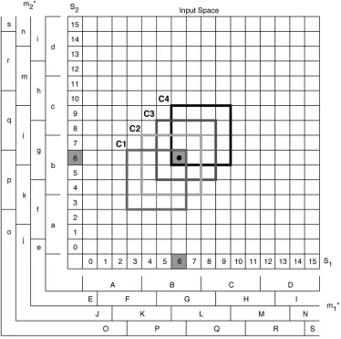
In the original implementation of the CMAC network [47], the memory cells of the network are divided into layers. The number of layers in a CMAC network is determined by the number ofquantization functionsdefined. That is, one quanti-zation function corresponds to one layer. Fig. 3 depicts an ex-ample of a two-input CMAC network with four quantization functions in each of the input dimensions. The resultant 2-D grid in Fig. 3 corresponds to the input space of the CMAC network that is used to learn the associative mapping patterns for 256 input–output (I/O) vector combinations. The quantization func-tions of the network are defined as follows.
Along dimension
(1)
Along dimension
(2)
where denotes the quantization function for the th layer of the th dimension and denotes the set of quantization levels. Each input vector selectsonememory cell from a layer. In the CMAC of Fig. 3, the input vector of (6,6) selects a total of four memory cells (one from each layer). That is, the , and cells that correspond to the quantization points of , and , respectively. The output of
the CMAC network is subsequently computed by the linear combination of the memory contents of the selected cells.
However, the multilayered structure of the CMAC network often renders the network operations difficult to comprehend. Moreover, in such an implementation, extensive layers of overlapping computing cells are required to produce a smooth output. The optimization of the memory allocation process (nonuniform quantization) of a multilayered, multi-input CMAC NN is not only tedious, but can also be computationally expensive, especially for high-dimensional input problems that require extensive layers of computing cells to achieve the desired output resolution or accuracy. This is because it is difficult to manipulate the distribution of the memory cells in the individual layers as the computation of all the overlap-ping layers are intertwined and tightly coupled to produce the CMAC output. Therefore, this paper proposes a single-layered CMAC implementation for the optimization of the memory allocation procedure based on hierarchical clustering. In such a computing structure, memory allocation or the distribution of the memory cells becomes manageable as there is only one layer of computing cells.
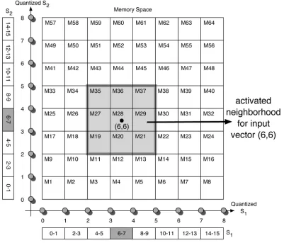
Fig. 4 illustrates such a single-layered perspective of a two-input CMAC network consisting of 64 memory cells. The 2-D computing grid corresponds to the memory space of the CMAC network. In Fig. 4, each of the input dimensions is uniformly
quantizedinto eight discrete quantization steps (or levels) for
Fig. 3. An example of a 2D CMAC network (m refers to the set of quantization functions along theS dimension andm refers to the set of quantization functions along theS dimension).
The conceptual similarities between the proposed single-lay-ered model and the original multilaysingle-lay-ered implementation of the CMAC network can be examined from their respective modeling principles. The layered cell activations in the original CMAC network contributed to the following two significant computational objectives: 1) smoothing of the computed output and 2) activating similar or highly correlated computing cells in the I/O associative space. These two modeling principles are similarly conserved in the single-layered model of the CMAC network via the introduction of a neighborhood-based computational process. The activation of the neighboring cells in the input space of the single-layered CMAC corresponds to the simultaneous activation of the highly correlated cells in its multilayered counterpart. This contributes to the smoothing of the computed output since the neighborhood-based activation process results in continuity of the network output. This activa-tion process will be further discussed in Secactiva-tion IV.
C. Nonuniform Quantization CMAC Variants
Several attempts to address the uniform quantization of CMAC can be found in the literature. In general, they can be classified into two main approaches based on the type of nonuni-formity introduced. The first approach uses layers/hierarchy of multiresolution CMAC networks to achieve nonlinearity
in memory storage allocation. Originally proposed by Moody [25], a CMAC is trained using coarsely quantized (low-resolu-tion) inputs. For regions where the error is large, the decision to add another CMAC with higher resolution is made. The expansion process continues until the error is reduced to an acceptable level. Some variations and applications of this type of nonuniform CMAC have also been proposed in [17] and [22]–[24]. While these methods can effectively capture the gen-eral trend as well as fine details in the ovgen-erall target function to be learned, the total number of memory cells needed to achieve a particular performance is not known in advance, making any hardware implementation awkward and difficult.
Fig. 4. Single-layer perspective of the 2-D CMAC network example shown in Fig. 3.
of the target function to be learned, which is often difficult to obtain or not known in advance. Furthermore, for these methods, the storage efficiency achieved is at the cost of significantly higher computational complexity. On the other hand, the adaptive quantization approaches proposed in [29] and [30] do not require the target derivative information. In [30], a data clustering algorithm is employed to find the centers of the partitions in the CMAC layers. In [29], the Shannon’s entropy measure is used to adaptively determine the information distribution of the training data. However, since entropy is measurable only for discrete/nominal inputs, this approach is more suited for classification problems.
Other CMAC variants such as the kernel CMACs [48]–[50] and the fuzzy CMACs [51], [52] do not employ quantization-based addressing schemes. In kernel CMAC, kernel functions such as B-spline kernels are used to derive the receptive fields of the network. While this method is able to reduce the memory re-quirement, the choice of kernel function is still an open problem. Moreover, the complexity of the resultant CMAC depends on the kernel function used. Fuzzy CMACs, on the other hand, employ input fuzzification methods to remove the sharp quan-tization boundary of the original CMAC network. The use of fuzzy inference schemes such as in [52] also enables the ex-traction of fuzzy rules from the trained network. While these variants offered the computational interpretability missing in the black-box CMAC model, there is a significant increase in the computational complexity of the hybrid network without a comparable performance gain.
IV. HCAQ-CMAC
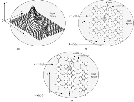
Fig. 5. Comparison of CMAC and HCAQ-CMAC memory structure for a particular target output surface. (a) I/O characteristic. (b) The 2-D CMAC memory structure. (c) The 2-D HCAQ-CMAC memory structure.
regions with relatively unchanged output values. As a result, a finer quantization level is obtained for the regions of the input space which contain more information. This nonuniform quantization process is illustrated in Fig. 5. Fig. 5(a) shows an example of a target output surface of a two-input problem to be modeled. Fig. 5(b) depicts the corresponding uniformly quantized CMAC memory structure and Fig. 5(c) illustrates the nonuniform HCAQ-CMAC for the same target output surface.
A. HCAQ-CMAC Network Architecture
Neurophysiological studies have established that the precise wiring of the adult human brain is not fully developed at birth [4]. Instead, there are two overlapping stages in the develop-ment of the human central nervous system. The embryonic stage of this process encompasses the formation of the basic archi-tecture of the nervous system, in which coarse connection pat-tern emerges as a result of the genesis and death of the brain cells during prenatal development. Subsequently, in the post-natal development stage, the initial architecture is refined and extraneous synaptic connections are pruned throughout an indi-vidual’s life-span by repeated exposures to various activity-de-pendent experiences. These processes constitute a selective al-location of neurons in the human brain and is incorporated to the HCAQ-CMAC memory allocation procedure as a mecha-nism for nonuniform quantization.
The HCAQ-CMAC memory allocation procedure is inspired by the biological development of the human central nervous system where neural cell death plays an integral part in the refinement process of the brain’s neuronal organization. In HCAQ-CMAC, the available memory cells are distributed based on the observed characteristics of the training data, which are defined by the data distribution in the input space as well as the variation of the target output value. For this reason, the HCAQ-CMAC architecture presented in this paper is a multiple-input–single-output (MISO) CMAC variant. This is because in a multiple-output domain, the variation of each output variable may not be correlated to one another. Thus, it is difficult to formulate a quantization function that is optimal for all output dimensions. A multiple-input–multiple-output (MIMO) problem can instead be modeled by a combination of several MISO systems.
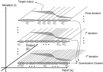
Fig. 6. Illustration of the HCAQ-CMAC nonuniform quantization process for an arbitrary input dimensionjwhereM = 6^ .
is employed at each dimension to identify the optimal quantiza-tion decision funcquantiza-tion in each of the input dimensions. A
quan-tization clusteris defined as the span of a memory quantization
level in a particular input dimension. Starting with the initial set of quantization clusters in a particular input dimension, two clusters with the smallest merging cost are combined in each it-eration of the hierarchical clustering process until the number of quantization clusters is equal to the number of available (pre-defined) memory space in the respective input dimension (see Fig. 6).
Let denote the total number of input dimensions for a given problem. Assume that a training data set of
is used to train the HCAQ-CMAC network, where denotesthe thinputvectortothenet-work and denotes the expected scalar output of HCAQ-CMAC. Let denote the total number of available memory cells per dimension and
denote a set of quantization clusters in the th input dimension at the th iteration of the hierarchical clustering process. The HCAQ-CMAC memory allocation process is described as follows:
Step 1) Perform data preparation. For each input
dimen-sion , the input training samples
’s are sorted in ascending order such that , where
.
Step 2) Define the initial set of quantization clusters. Let denote the th quantization cluster in the th input dimension at the th iteration of the hierar-chical clustering process, and as the number
of data points in . Then, the quantization cluster is defined as the set of I/O data pairs such that
.Foreachinputdimension , where , the initial set of quantization clusters is derived from the input training data
points in the th input dimension.
Eachdistinctinput value from the training set
constitutesonequantization cluster in the th dimen-sion. Training data points with the same input value are combined together as a cluster such that
(3)
where
. Each quantization cluster is defined by a characteristic value and its centroid . The characteristic value of a quantization cluster at the th iteration of the hierarchical clustering process is computed as the mean of the output values of the input points and is described by
(4)
where is the total number of data points in the quantization cluster at the th iteration. , on theotherhand,denotesthecentroidofthequantization cluster and is described by
With respect to the input dimension , the ini-tial set of quantization clusters is defined as
where
and and
(since ).
Step 3) Merge similar quantization clusters iteratively. The clusters in the initial set of quantization clusters are iteratively merged until the number of quantiza-tion clusters in the th dimension is equal to the number of predefined available memory cells, i.e., . Only the two most similar adjacent clusters can be merged in each iteration. The cluster-merging decision is based on acost function. The merging cost function is defined as the weighted combination of the distances between the characteristic values and the centroids of two adjacent clusters, and is described mathematically in
(6)
(7)
where is the merging cost of the two adjacent clusters and (i.e.,
and ) at the th iteration, and and are user-defined parameters. The pa-rameters and weight the respective importance of the measured differences in the output (character- isticvalues)andtheinput(quantizationpoints)dimen-sions as the total cost of merging two adjacent clus-ters.Theweightingparameter isconcernedwiththe similarity of the outputs of the two clusters. , on the otherhand,controlstheimportanceofthesimilarityof the inputs in the two clusters. As such, the selection of and parametersgenerallyvariesgreatlywithdif-ferent applications and may be guided by the relevant prior knowledge about the applications or the training data. An application with slow changing input but fast changing output may require a bigger than and vice-versa.
In each iteration, the two adjacent clusters with the smallest merging cost are combined as in
iff
(8)
The characteristic value and the centroid of the merged cluster are recom-puted using (4) and (5). The cluster-merging process
continues until the number of clusters in the input di-mension reachesthepredefinedmemorysize (see Fig. 6). This is analogical to the activity-dependent pruning of the extraneous synaptic connections in the human brain. Weak (or nonactive) neurons are elimi-nated and their functions annexed by the winning (or more active) neurons. In the HCAQ-CMAC, similar clusters are merged and represented by larger/ex-panded clusters to reduce data redundancy. Specifi-cally, HCAQ-CMAC allocates more memory cells to the densely data-populated areas with higher degrees of output variation.
Step 4) Construct the quantization decision function. A set of quantizationclustersisobtainedattheendofthehi-erarchicalclusteringprocessforeachinputdimension . Let denote the last cluster-merging iteration for input . Thus, the final set of quantization clusters for
input isdefinedas .
Subsequently, the quantization decision function in the th input dimension is determined from
, as described by
(9)
where denotes the quantization mapping func-tion in the th input dimension. is the centroid of the th quantization cluster of the th input dimen-sion after the cluster-merging process and is the number of predefined memory cells in each dimen-sion. The quantization decision points derived for each input dimension subsequently form the memory axes of the HCAQ-CMAC network and define its overall computing structure.
B. HCAQ-CMAC Operating Principles
The HCAQ-CMAC network learns a correct response to an input vector by modifying the contents of the selected memory cells. Let be the maximum number of training iter-ations. The Widrow–Hoff learning rule [54] is adopted and the HCAQ-CMAC memory learning process for the th training sample is described as follows.
Step 1) Determine the winner neuron for input at the th iteration, where . For each input , the index of the winner neuron in HCAQ-CMAC is computed via the quanti-zation mapping functions . That is, given , the winner neuron is as in
(10)
where denotes the quantized input and is the number of input dimensions.
training iteration is the memory content at the loca-tion . This is described by
(11)
where denotes the HCAQ-CMAC output for the input during the th training iteration and is the HCAQ-CMAC hypercube memory array. Step 3) Compute the network output error. The learning
error corresponding to the input at the th training iteration is defined as the difference between the network output and the expected output is given in
(12)
Step 4) Update the HCAQ-CMAC memory. The update equation for the activated cell at index is given by
(13)
(14)
where denotes the learning constant.
During the testing phase of the HCAQ-CMAC network, a neighborhood-based activation of the network cells is employed to smoothen the computed output. Given an input stimulus to the HCAQ-CMAC network, the network output during the testing phase is derived as follows.
Step 1) Determine the region of activation. The computed output of the HCAQ-CMAC network corresponding to an input stimulus is defined as the mean of the memory contents (values) of the activated cells in the neighborhood vicinity of . The neighbor-hood of is defined by a neighborhood constant , which determines the relative size of the neigh-borhood with respect to the input domain. For an input stimulus , its activation neighborhood is de-fined by
range (15)
range (16)
where denotes the th input
di-mension, is the neighborhood constant, range is the input domain for the th dimension, is the left boundary of the neighborhood in the th dimension, and is the right boundary of the neighborhood in the th dimension. Consequently, the memory cells within the neighborhood consti-tute the set of activated computing cells for the input stimulus . The size of the neighborhood affects the accuracy of the computed HCAQ-CMAC output. The larger the neighborhood size, the more gener-alized is the output of the HCAQ-CMAC network. Conversely, a smaller neighborhood size results in a more accurate output computation. Therefore, a
larger neighborhood size is suitable for a data set that is sparse in the input space as this increases the gen-eralization ability of the HCAQ-CMAC network. A smaller neighborhood size, on the other hand, is suit-able for a compact data set so as to produce more accurate results.
Step 2) Compute the HCAQ-CMAC output. The output of the HCAQ-CMAC network with respect to the input
is defined by
(17)
where denotes the set of indexes of the activated neighborhood cells corresponding to the input , is the memory content of the activated cell with index , is the cardinality of , and is the output of HCAQ-CMAC with respect to the input stimulus .
As a computational model of the human cerebellum, the pro-posed HCAQ-CMAC network possesses characteristics analog-ical to the neurobiologanalog-ical and neurophysiologanalog-ical aspects of its biological counterpart. Appendix A lists the neural correlates between the human cerebellum and the HCAQ-CMAC network.
V. HCAQ-CMAC LEARNINGCONVERGENCE
This section presents the mathematical proof of the learning convergence of the proposed HCAQ-CMAC network. Fig. 7 depicts an example of the memory surface of a two-input HCAQ-CMAC network. With respect to Fig. 7, the quantization points along the dimension are
and along the dimension are ,
re-spectively. denotes the network cell with the address
index .
A. Mathematical Perspective of the HCAQ-CMAC Network The HCAQ-CMAC network employs a winner-take-all learning principle where each input training tuple accesses and modifies the memory content ofonewinner neuron. Each input vector to the network is quantized to the nearest quantization level in each dimension to identify the index of the winner neuron. The HCAQ-CMAC network output is derived from the winner network cell. Consequently, the network learning process is performed on this winner cell.
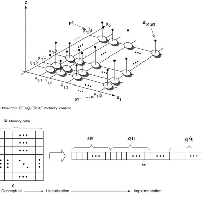
The conceptual memory surface of a multiple-input HCAQ-CMAC network can be expressed as a 1-D weight array . Fig. 8 illustrates the linearization of the concep-tual memory surface to the physically implemented 1-D weight array for a 2-D HCAQ-CMAC. With respect to the HCAQ-CMAC network, the computed output for the th input vector (stimulus) is defined in
(18)
where is the training iteration number, denotes the quan-tization mapping function of the HCAQ-CMAC network, and is the index to the winner neuron corresponding to the input .
Fig. 7. Example of the two-input HCAQ-CMAC memory content.
Fig. 8. The 2-D HCAQ-CMACZ ! Wmapping.
HCAQ-CMAC network be and the column vector [see (19)] denote the activation mask of the HCAQ-CMAC memory cells with respect to the th input training sample. That is
array
(19)
if the th memory cell is activated
otherwise (20)
Note that the winner-take-all learning algorithm of the HCAQ-CMAC network implies that, for all , only one ele-ment of is nonzero. The scalar output of the HCAQ-CMAC network can thus be formulated as a vector product described by
array
(21)
where is the memory content of the entire HCAQ-CMAC network structure when the th input training sample is pre-sented.
The memory update equation of the HCAQ-CMAC network for the th input training sample is subsequently defined as
local error learning error
local error
(22)
where
the memory content of the entire HCAQ-CMAC network structure when the th training sample is presented in the th training iteration;
the learning constant;
the activation mask of the HCAQ-CMAC memory cells;
The difference of the HCAQ-CMAC memory contents be-tween two successive iterations for the th input training sample (denoted as ) is, therefore, defined as
(23)
Note that the activation mask is a constant for an arbitrary input training sample across different training iterations. This is because the HCAQ-CMAC network structure is static after the structural learning phase.
Following (23), the delta memory contents for a sequence of
training data is described by
(24) and
(25)
where denotes the total number of training samples.
The learning convergence of the HCAQ-CMAC network is established via the convergence of the network memory contents as training approaches infinity. In this case, the sufficient and necessary condition for the HCAQ-CMAC learning process to convergence can be expressed in
(26) or
(27)
where is the null matrix. Substituting (24) into (23)
(28)
The HCAQ-CMAC network is iteratively trained on a set of training samples. When , from (28)
(29) such that
(30) and
[from (24)] (31)
Following the results of (28)–(31), [see (25)] can be re-expressed as
(32)
Decomposing the terms on the right-hand side repeatedly results in
(33)
Following (33):
(34) Therefore, (33) can be reexpressed as
(35)
It can be observed that
Consequently, it follows that
(37)
Further repeated decomposition of the terms on the right-hand side results in the following:
(38)
With respect to (38), the memory difference matrix must approach a null matrix as training tends to infinity (i.e.,
) in order to establish the learning convergence of the proposed HCAQ-CMAC network. Hence, the HCAQ-CMAC learning process converges if and only if (39) holds
(39)
By definition, the difference vector can be expressed as
(40)
Decomposing the terms on the right-hand side repeatedly produces
(41)
From (22), the HCAQ-CMAC memory update due to the th input training sample at the th iteration is computed via
learning error
local error
(42)
where is a scalar value and it is the learning (training) error of HCAQ-CMAC for the th input training vector at the th iteration. If
(43)
then (42) can be reexpressed as
(44)
From (38), (41), and (44)
(45)
Therefore, if for all
in (45) evaluates as null.
From (38), the matrix as follows.
Conse-quently, the learning process of the proposed HCAQ-CMAC network converges.
B. Learning Convergence of the HCAQ-CMAC Network
Theorem 1: The training process of the HCAQ-CMAC
net-work converges if and only if the learning constant is such
that .
Proof: It can be shown that for all , when
, (reefer to Appendix B for
a detailed proof). Therefore, the training process of the HCAQ-CMAC network converges if and only if the learning constant satisfies the condition .
VI. EXPERIMENTALRESULTS ANDANALYSIS
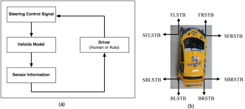
Fig. 9. Simulation environment. (a) Vehicle control sequence. (b) Car sensor placements.
network [25] to assess the generalization and learning ability of the proposed network, and 3) Menozzi’s tree-based multires-olution CMAC [24] to assess both the modeling performance and memory efficiency achievable by HCAQ-CMAC.
A. Automatic Control of Car Maneuver
Theintelligent vehicle projectis part of an ongoing research
effort to develop an intelligent transportation system (ITS) at the Centre for Computational Intelligence (C2i), Nanyang Techno-logical University, Singapore[55]. The objective of the project is to realize brain-inspired intelligent-based technologies required for the automation of control, routing, and navigation of land ve-hicles. In this paper, the proposed HCAQ-CMAC network is em-ployed for the construction of an autopilot system for car ma-neuver. Albeit its complexity, driving a vehicle is a motor task that humans are able to perform relatively well. It has been well estab-lished that the learning of motor skills is mediated by the human
procedural memory system[56], which consist of the cerebellum
and the striatum (part of basal ganglia formation). The human procedural memory system is a facet of the brain’s information processing capacity specifically for the acquisition of skilled be-haviors and habits. Vehicle driving comprises of finely tuned sets of sensory feedback to control action mappings that are accumu-lated through experiences and repeated practices. Although hu-mans are quite adept at mastering complex skills, it is difficult to formalize these behaviors into mathematical algorithms. In such cases, the construction of a computational model that is able to emulate the functionality of the human brain is required [57]. This subsequently motivates the use of HCAQ-CMAC to model and emulate the human driving expertise.
In this experiment, a driving simulator (as developed in [58]) is employed to capture the behavioral response of the human driver. The simulator consists of a 3-D virtual driving environment that integrates a detailed model of the vehicle dynamics and engine characteristics together with the environmental parameters such as road profiles. The approach to the experiment is to capture and record the driving data of a human driver, which consists of a set of distance-sensor feedback information and the corresponding steering control performed by the human driver as he maneu-vers the simulated car around a specified track. The feedback
sig-nals provide information such as the distance of the vehicle from the road boundaries. The simulator allows for vehicle control via steering adjustment. An overview of the driving control sequence is given in Fig. 9(a). These feedback-control records are then used to train the HCAQ-CMAC-based autopilot system.
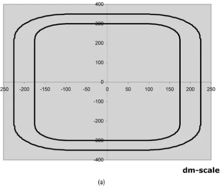
The objective of the autopilot system is to control the vehicle to follow a particular lane in a multilane circuit track. The simulated vehicle model is equipped with eight directional sensors as shown in Fig. 9(b). The semantics of the sensor readings are tabulated as Table I. For the autopilot system, only the front four sensors are utilized [i.e., SFLSTB, FLSTB, FRSTB, SFRSTB; Fig. 9(b)] as the inputs to the HCAQ-CMAC network. As an output, the network responds with the appro-priate steering angle. Two tracks are used in this experiment. The HCAQ-CMAC autopilot system is first trained on track 1 [Fig. 10(a)], with the car traveling in both clockwise and counterclockwise direction. Subsequently, track 2 [Fig. 10(b)] is used for testing. The simulated track is 5 m wide.
The training data set (recorded from a human driver) contains 1018 samples. HCAQ-CMAC and the benchmarked systems were trained within 500 training epochs with a network learning constant of 0.1. Table II outlines the performances of the HCAQ-CMAC autopilot system as compared to the following: 1) the basic CMAC network, 2) Moody’s multiresolution CMAC net-work, and 3) the tree-based multiresolution CMAC network. Each simulation test result was collected over 100 s of driving-time, with a maximum driving speed of 100 km/h. The driving performances of the various networks were measured by the av-erage deviation of the controlled car from the center of the lane (ACD) and the average deviation of the car orientation from the desired orientation (AOD). Both the ACD and AOD mea-surements are subsequently normalized and reported as normal-ized ACD (NACD) and normalnormal-ized AOD (NAOD). NACD de-notes the ACD with respect to the half track width, which is the maximum leeway available before the car collides with the road boundaries. The AOD values are normalized with respect to radians. A performance index (PI ) is used to combine the NACD and NACD measures as described in
PI NACD NAOD (46)
Fig. 10. Driving tracks. (a) Training track (track 1). (b) Testing track (track 2).
TABLE I
SENSORSDEFINITION OF THECARSIMULATOR
where PI is the normalized PI . Thus, a higher PI value cor-responds to a better network performance.
For the simulation, a learning constant of 0.1 and a neighbor-hood constant of 0.2 were empirically determined for the eval-uated networks. The network size is also varied to determine the optimal performance for each of the networks. Based on the PI values in Table II, the basic CMAC network achieved an optimal performance with a memory size of ten memory cells per dimension. For CMAC, a small network size results in a coarse partitioning of the input space, and hence, the net-work suffers from anaveraging effect. A large CMAC network, however, fails to generalize from the available training data and thus performs poorly on the testing track. The multiresolution CMAC architectures, on the other hand, employ layers of over-lapping CMAC networks with different resolutions to address the generalization-accuracy dilemma. Both Moody’s multires-olution CMAC (MMR-CMAC) and the tree-based multireso-lution CMAC (TMR-CMAC) architectures were benchmarked using two- and three-layers implementations. These overlay im-plementations improve the generalization ability of the finer res-olution CMACs while simultaneously maintaining their output accuracy, but at the expense of higher memory requirements. Best PI values were observed for a two-layer MMR-CMAC with memory size of five cells per dimension for the first layer and ten cells per dimension for the secondary layer, and a two-level TMR-CMAC employing a CMAC of size eight cells per
dimension at the first level and 26 CMACs of size two per di-mension at the second level.
From the results presented in Table II, one can observe that the proposed HCAQ-CMAC-based autopilot system consis-tently outperformed the other three CMAC architectures. An optimal HCAQ-CMAC network performance is obtained with a memory size of only five cells per dimension with a PI value of 172. The hierarchical clustering technique of the HCAQ-CMAC network effectively allocates the available memory cells to the input regions with high utilization throughput. This ensures that more cells are allocated to important input regions that contain more information. Therefore, a small network size does not affect the accuracy and fine-tuning capability of the HCAQ-CMAC network. Moreover, with a smaller network size, fewer cells in HCAQ-CMAC are allocated to areas with little or no training data, thus improving the generalization ability of the network. The efficient memory allocation scheme of HCAQ-CMAC also reduces the required network training time. The best-performing HCAQ-CMAC network trains in the shortest time (i.e., 7562 ms) among all the benchmarked networks. Subsequently, the effective cell utilization rates of the various networks were computed and the results [denoted as the cell occupancy rate (COR)] are tabulated in Table III. The COR is defined as the proportion of the trained network cells to the total network size. From Table III, one can observe that the HCAQ-CMAC network achieves the highest COR value in comparison with the other three CMAC architectures. This clearly demonstrated the effectiveness of the proposed HCAQ-CMAC memory allocation scheme.
B. Modeling the Dynamics of the Human Glucose Metabolic Process
TABLE II
COMPARISON OFRESULTS FOR THEVARIOUSCMAC NETWORKSUSING THEAUTOPILOTSYSTEM
hypoglycemia can deprive the body of energy and causes the patient to lose consciousness, which can eventually become life threatening. Currently, the treatment of diabetes is based on a two-pronged approach: strict dietary control and insulin medication.
The key component to a successful management of diabetes is essentially to develop the ability to maintain a long-term
near-normoglycaemiastate of the patient. With respect to this
objec-tive, the therapeutic effect of discrete insulin injections is not ideal as the regulation of insulin is an open-looped process. Con-tinuous insulin infusion through an insulin pump, on the other hand, is a more viable approach due to its controllable infusion rate [59]. Such insulin pumps are algorithmic-driven, with an avalanche of techniques proposed, investigated and reported in the literature over the years [60], [61]. Generally, all such pro-posed methods required some forms of accuratemodeling of the glucose metabolic process of the diabetic patient before a suitable control regime can be devised.
In recent years, emerging evidences have suggested that glucose metabolism throughout the body is coordinated by the brain through the use of insulin [62]. This is reinforced by the fact that glucokinase, the established glucose sensor of the pancreatic -cells, is observed to be also present in the central nervous system (CNS) [63]. Precise experimentations have subsequently demonstrated that insulin, via acting on the hypothalamus (a subcortical brain structure central to the autonomic control of the human endocrine system), exerts a
high level of supervisory control on glucose production by the liver [64]. This observation contemplates that insulin can mediate the human glucose metabolic process through an un-known signaling pathway via the CNS [65], [66]. This notion subsequently motivates the use of the HCAQ-CMAC network, which is a brain-inspired computational model of the human cerebellum, for the dynamic modeling of the human blood glucose cycle.
The first step into constructing a model of the human glucose metabolic process is to determine the patient profile to be mod-eled. Due to the lack of real-life patient data and the logistical difficulties and ethical issues involving the collection of such data, a well-known web-based simulator known as GlucoSim [67] from the Illinois Institute of Technology (IIT, Chicago, IL), is employed to simulate a person subject to generate the blood glucose data that is needed for the construction of the glucose metabolism model. A person profile for the simulated healthy subject is created as shown in Table IV.
TABLE III
COMPARISON OFCORS FOR THEVARIOUSCMAC NETWORKS
TABLE IV
PROFILE OF THESIMULATEDHEALTHYPERSON(SUBJECTA)
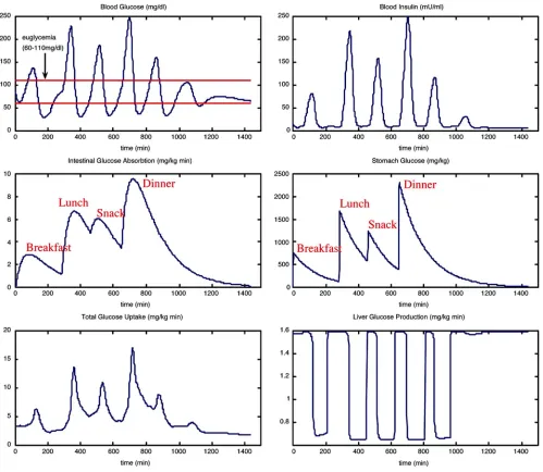
Fig. 11 illustrates a sample output from GlucoSim for subject A. This output consists of six elements: blood glucose, blood in-sulin, intestinal glucose absorption rate, stomach glucose, total glucose uptake rate, and liver glucose production rate of subject A, respectively, over a simulated time period of 24 h. The peaks in the stomach glucose subplot of Fig. 11 coincide with the tim-ings of the assumed four daily meals (i.e., breakfast, lunch, after-noon snack, and dinner) while those peaks in the intestinal glu-cose absorption rate subplot reflect a delay effect (response) of food intake on the blood glucose level of subject A. The subplots of blood glucose and blood insulin illustrate the insulin–glucose regulatory mechanism in a healthy person such as subject A and depict the dynamics of the metabolic process when subjected to disturbances such as food intakes.
Since the human glucose metabolic process depends on its own current (and internal) states as well as the exogenous food intakes, it is hypothesized that the blood glucose level at any given time is a nonlinear function of prior food intakes and the
historical traces of the insulin and blood glucose levels. To prop-erly account for the effects of prior food ingestions to the fluc-tuation of the blood glucose level, a historical window of 6 h is adopted to trace the carbohydrate content of the meals taken. A soft-windowing strategy is employed to temporally partition the 6-h historical window into three conceptual segments, namely,
recent(i.e., previous 1 h),intermediate past(i.e., previous 1–3
h), andlong ago(i.e., previous 3–6 h). Based on these windows, three normalized weighting functions are introduced to compute the carbohydrate content of the meal(s) (with respect to current time) taken recently, in the intermediate past or long ago. Thus, inclusive of the measured blood glucose and insulin levels, there is a total of five inputs to the modeling task. Fig. 12 depicts the weighting function for each of the respective segmented win-dows.
Fig. 11. Sample glucose metabolism data output from the GlucoSim simulator.
as the TMR-CMAC network. For this application, a neighbor-hood constant of 0.1 and a learning rate of 0.1 are empirically determined. Table V details the recall (training) and generalization (testing) performances of the various networks with different network sizes. Two performance indicators are employed to quantify the modeling quality of the networks: the root-mean-squared error (RMSE) and thePearson correlation
coefficientbetween the actual and the computed blood glucose
level. The RMSE and Pearson correlation measures were subsequently employed to compute the PI described by
PI Pearcorr
RMSE (48)
Therefore, a higher PI value reflects a better network modeling performance.
Due to the characteristics of the training data, the perfor-mances of the networks vary with their respective network sizes. From the PI values in Table V, one can observe that for the
Fig. 12. Soft-windowing weighting functions to compute the carbohydrate content of meal(s) in the segmented windows of the 6-h food history. (In the figure, the current time is 1840 h and there are three instances of food intakes in the previous 6 h; that is, lunch at 1245 h, afternoon snack at 1524 h, and dinner at 1833 h, respectively.)
TABLE V
COMPARISON OFRESULTS FOR THEVARIOUSCMAC NETWORKS ON THEMODELING OFGLUCOSEMETABOLISMPROCESS
MMR-CMAC via the addition of the middle-layer CMAC. On the other hand, even though the TMR-CMAC network also em-ployed layers of CMAC networks of different resolutions, its performances were found to be relatively poor in comparison to the other benchmarked networks. This may be due to the overlay mechanism of the TMR-CMAC, where finer resolution CMACs are selectively allocated to the input subregions with large output errors. The resolutions of these CMACs are in-creased as required and only the finest resolution layers are kept. On the other hand, an optimal PI value (generalization) was achieved by the HCAQ-CMAC network with a memory size of ten cells per dimension. This HCAQ-CMAC network managed to produce a rather good fit to the actual blood glucose profile as indicated by a high correlation value of 97.48% and a relatively low RMSE of 10.4312 mg/mL of blood glucose concentration. There are only slight improvements in the HCAQ-CMAC
Fig. 13. Modeling results of the CMAC and HCAQ-CMAC network for the glucose metabolic process of subject A. (a) Generalization performance of CMAC network (size=ten cells per dimension). (b) Generalization performance of HCAQ-CMAC network (size=ten cells per dimension).
addition, the proposed HCAQ-CMAC network achieved com-parable recall and generalization performances, which demon-strates that the network is able to efficiently extract the inherent relationships from the training data.
To further analyze the performance of the HCAQ-CMAC net-work, a three-days modeling result of the CMAC and HCAQ-CMAC networks (each of size ten cells per dimension) are de-picted in Fig. 13. Fig. 13 clearly demonstrated the generalization and modeling accuracy of the HCAQ-CMAC network. Due to the nature of the training data, the static uniform quantization of the basic CMAC network resulted in an abundance of untrained network cells as evidenced in Fig. 13(a) (the effects of the un-trained network cells are highlighted as , and , respec-tively). The HCAQ-CMAC network, on the other hand, is able to selectively allocate the available memory space according to the information distribution of the training data, and thus, signif-icantly reduces the number of untrained network cells to facili-tate a consistent modeling performance as evident in Fig. 13(b).
VII. CONCLUSION
This paper presents a novel brain-inspired nonuniformly quantized CMAC architecture named the HCAQ-CMAC net-work. Inspired by the physiology of the human cerebellum,
as well as the neurobiological mechanisms of the neuronal selection process underlying human brain development, the HCAQ-CMAC network employs an information-driven memory allocation scheme.
TABLE VI
CORRESPONDENCEBETWEEN THENEUROPHYSIOLOGICALASPECTS OF THEHUMANCEREBELLUM AND THEFUNCTIONALITIES OF THEPROPOSEDHCAQ-CMAC NETWORK
as reflected by the considerably higher CORs observed in the car-driving experiment.
However, even though HCAQ-CMAC reports relatively higher CORs, memory efficiency remains at less than 12%. This is mainly due to the fact that the quantization process of the HCAQ-CMAC is separately performed in each input dimension. This is to reduce the computational complexity arising from the introduction of nonuniform quantization to the CMAC network, and work reasonably well for low-di-mensional problems but may cause large memory wastage for higher dimensional problems. Research efforts are currently directed at addressing this limitation. Currently, the memory sizes employed in the applications have been empirically deter-mined. This is because depending on the data characteristics, different applications require different memory sizes to achieve an optimal performance. The hierarchical clustering technique employed in the HCAQ-CMAC network does not possess the ability to automatically determine the optimal number of quan-tization clusters. Instead, this paper concentrates on achieving maximum performance with the available (predefined) number of memory cells. A future enhancement to HCAQ-CMAC is to extend the architecture to support online learning. Currently, since the result of the hierarchical clustering technique is static, HCAQ-CMAC is not suitable for online training. To address this drawback, a change of clustering technique may be necessary.
As future work, the HCAQ-CMAC-based human blood glu-cose model would be used in the development of a blood gluglu-cose prediction system for diabetes treatment. Future applications of
the HCAQ-CMAC network also includes various pattern recog-nition tasks [69]–[71], financial engineering [72], and biomed-ical domain [73]. Currently, these research endeavours are ac-tively underway at the C2i [55]. The C2i lab undertakes intense research in the study and development of advanced brain-in-spired learning memory architectures [74]–[78] for the mod-eling of complex, dynamic, and nonlinear systems. These tech-niques have been successfully applied to numerous novel ap-plications such as automated driving [58], signature forgery de-tection [79], gear control for the continuous variable transmis-sion (CVT) system in an automobile [80], fingerprint verifica-tion [81], bank failure classificaverifica-tion and early warning system (EWS) [82], computational finance [83], [84], as well as in the biomedical engineering domain [85], [86].
APPENDIXA
HCAQ-CMAC NEURALCORRELATES
See Table VI.
APPENDIXB
PROOF OFLEARNINGCONVERGENCE
This section provides the mathematical proof of the
expres-sion for all , given that the
learning constant satisfies the condition .
and the activation mask of the HCAQ-CMAC network for the th input training vector as
array
if the th memory cell is activated otherwise
the matrix has the following properties.
Property 1: is a symmetric matrix.
Proof:
Thus, is a symmetric matrix.
Property 2: Let matrix be denoted as . The
diagonal elements of matrix can be expressed as
if th element of is if th element of is
and the nondiagonal elements of matrix are always zero, i.e.,
Proof: According to the definition of the activation mask
, as well as from the principle of the winner-take-all learning algorithm of HCAQ-CMAC, there will only be one nonzero el-ement in for the th input training vector. Consequently, as the matrix is defined as
it follows that
if th element of is if th element of is
and is 0 for all .
Lemma 2: Let the matrix be the multiplication result for
any arbitrary matrix and the matrix such that
where is a matrix. If the learning rate satisfies the condition , then the -norm of any arbitrary th row vector in will be bounded by the -norm of the corresponding th row vector in . That is
row of row of if
Proof: Let the matrix be denoted as
and matrix be denoted as , respectively. The -norm of the th row vector of is evaluated as
row of
On the other hand, the -norm of the th row vector of can be derived as
row of row of
From Property 2, it is established that all of the nondiagonal elements of the matrix evaluate as zero. Furthermore, of all the diagonal elements of the matrix , exactlyoneelement is equal to . Let this element be at the th position in the activation mask, i.e., . Substituting the value of into the -norm of the th row vector of yields
row of
row of row of
For row of row of , the term
has to be less than or equal to 0, i.e.,
always when
Lemma 3: Following Lemma 2, if the learning constant
satisfies the conditions and , then the
-norm of any arbitrary th row vector in will always be smaller than the -norm of the corresponding th row vector in . That is
row of row of
if and
Furthermore, given that the learning constant satisfies the con-dition , the -norm of any arbitrary th row vector in will be equal to the -norm of the corresponding th row vector in if and only if , where denotes the position of the winner neuron in the activation mask , i.e.,
if row of row of
iff and
Proof: From Lemma 2, it has been established that if the
learning constant satisfies the condition , then row of will not be greater than row of . It follows that of Lemma 2 is always less than
zero if and , where denotes the position
of the winner neuron in the activation mask . Hence
row of row of
if and
Consequently, the condition of
row of row of
will holdif and only if for .
Lemma 4: If the learning constant satisfies the condition
, then the -norm of any arbitrary th row vector in is bounded by the -norm of the corresponding th row vector in . That is
row of row of
Furthermore, as the training iteration approaches infinity
row of
where denotes the entire set of the training data and is the set of indexes of the trained cells in HCAQ-CMAC due to
.
Proof: From the definition of the matrix [see (34)]
terms
where is the total number of input training samples and is a matrix. From Property 2 (Lemma 1), is a diagonal matrix such that
if if
where is the index of the activated cell in . Hence, is also a diagonal matrix.
From Lemma 3,
row of row of row of
row of
row of row of
Note that row of if is an
untrained cell. On the other hand, if , it follows from
Lemma 3 that row of row of as
and . Following from aforementioned, as the training iteration tends to infinity
row of
Lemma 5: If the learning constant satisfies the condition
, then as the training iteration tends to infinity and the term converges to a null matrix for all
. That is
if
Proof: From Lemma 4
row of
Hence, it follows that
if
REFERENCES
[1] F. A. Middleton and P. L. Strick, “The cerebellum: An overview,”
Trends Cogn. Sci., vol. 27, no. 9, pp. 305–306, 1998.
[2] J. S. Albus, “Marr and Albus theories of the cerebellum: Two early models of associative memory,” inProc. IEEE COMPCON, 1989, pp. 577–582.
[3] J. S. Albus, “A theory of cerebellar function,”Math. Biosci., vol. 10, no. 1, pp. 25–61, 1971.
[4] E. R. Kandel, J. H. Schwartz, and T. M. Jessell, Principles of Neural Science, 4th ed. New York: McGraw-Hill, 2000.
[5] D. Marr, “A theory of cerebellar cortex,”J. Physiol. London, vol. 202, pp. 437–470, 1969.
[6] J. S. Albus, “A new approach to manipulator control: The cerebellar model articulation controller (CMAC),”J. Dyn. Syst. Meas. Control, pp. 220–227, 1975.
![Fig. 1. Schematic diagram of the cerebellum (adapted from [2]).](https://thumb-us.123doks.com/thumbv2/123dok_us/8440315.334207/3.594.101.493.63.248/fig-schematic-diagram-cerebellum-adapted.webp)
![Fig. 2. Schematic diagram of the CMAC NN (adapted from [2]).](https://thumb-us.123doks.com/thumbv2/123dok_us/8440315.334207/4.594.105.484.64.282/fig-schematic-diagram-cmac-nn-adapted.webp)