C-T
OOL
version 1.1
A TOOL FOR SIMULATION OF SOIL CARBON
TURNOVER
Description and users guide
Bjørn Molt Petersen
June 2003
Danish Institute of Agricultural Sciences
Department of Agroecology
Research Centre Foulum
P.O. Box 50, DK-8830 Tjele
Denmark
Contents
1. Introduction 2. Model description
2.1. Carbon pools
2.2. Rate and allocation modifiers 2.3. Isotope simulation
2.4. Steady level 3. Input files
3.1. Mandatory input files 3.1.1. Control file
3.1.2. Model structure file 3.1.3. Initialisation file
3.1.4. Added organic matter file 3.1.5. Supply file
3.2. Optional input files 3.2.1. Microclimate file 3.2.2. Radiocarbon file 4. Output files
5. Installation and execution of the program 5.1. Installation
5.2. Execution
6. Execution examples for 3-pool model 6.1. Input file examples
6.2. Execution results
1. Introduction
The program C-TOOL (v. 1.1) can enhance SOM model development by aiding the
construction, revision and testing of soil carbon turnover models. Models can be created directly, without the aid of programmers. The program can use any time step between one day and one year, and can be run either for a predefined period or continue until specified steady-level criterions for carbon pools are reached. Development in soil carbon content at any desired time span can be simulated.
Simulation of carbon isotopes 13C and 14C is facilitated, and it is possible to simulate a specific isotope tagging in order to investigate carbon flow properties in the implemented model.
Standard driving variables are temperature (in air or soil), soil water content (either absolute content, relative content or pressure potential) and amount, type and application date for input of carbon to the soil.
All settings are performed through ascii-files, and not through screen dialogs.
2. Model description
A description of the scientific rationale behind this software is provided by (Petersen et al., 2002).
2.1. Carbon pools
The decay of carbon in each pool is described by first-order reaction kinetics dC
dt k C
i
i i
= − (1)
where ki is the decay rate coefficient for pool i (time-1), and Ci is the carbon content in pool i (amount). The specific unit will depend on the actual model specification.
The model is by default updated in discrete steps (Euler integration) by subtracting Di∆t from
Ci, where ∆t is the time step (time). The decay rate Di of pool i (amount C time-1) is by default
calculated as
Di =k Ci i (2)
As an option set by the user, the decay rate can alternatively be calculated as
An optional fourth order Runge-Kutta integration method is implemented. The use of this will yield better accuracy, at the cost of execution speed. It should only be used in combination with Eq. 2, not with Eq. 3.
The preferable method depends on the specific application and the time step. Under most circumstances, the difference between the methods will be negligible with a daily time-step, but with larger time-steps the Runge-Kutta integration in many cases may be preferable.
Three types of SOM-pools are distinguished: 1) added organic matter, 2) microbial biomass, and 3) native soil organic matter.
Microbial biomass pools have additional maintenance (Mi) and utilisation efficiency (Ei)
components. The fraction 1-Ei of the incoming carbon is lost from the system as CO2. The
maintenance (CO2 loss) is calculated by Eq. 2 or 3, substituting ki with Mi.
Added matter pools have associated sub-pools with decay rates that can depend on the type of added matter.
The calculations within each time step are made in the following order: 1) the decay of all pools is calculated, 2) the decay is directed to other pools and/or lost as CO2 as specified by the
model structure file.
2.2. Rate and allocation modifiers
The decomposition rate can be set to depend on several abiotic and biotic functions. The standard set up is:
ki k F T F W F Xis
T W X
= ( ) ( ) ( ) (4)
where ki is the actual decay rate for pool i (time-1), ki
s is the decay rate (time-1) at standard
conditions, FT is a function of temperature T (°C), FW is a function of soil water content W, and FX
is a function of clay content X (fraction). Any of the three modifier functions in Eq. 4 can optionally be left out.
The standard temperature dependency (after Kirschbaum, 1995), is
( ) exp[ (1 0.5 / )]
T m
F T = A α β+ T − T T (5)
where A (dimensionless) by default is adjusted to give unity output at 10 °C, α has a default value
of –3.432, β has a default value of 0.168 °C-1, and Tm has a default value of 36.9 °C.
( )
exp ( )( 273.2)( 273.2)
r T
r T T
F T A
T T
ω
−
=
+ +
(6)
Default values are: ω: 6352.0 °K, Tr: 30.0 °C, A (dimensionless) is default adjusted to give unity
output at 10 °C.
( ) /10 10
( ) T Tr
T
F T = AQ − (7)
Q10 represents the increase in the turnover rate for a temperature increase of 10°C, default value 2,
A (dimensionless) is default adjusted to give unity output at 10 °C.
2
0 0
( ) 0.1 0 20
exp(0.47 0.027 0.00193 ) 20
T
T
F T AT T
A T T T
≤
= > ≤
− + >
(8)
By default A (dimensionless) is 1.
0 18.3
47.9
( ) 18.3
106
1 exp( )
18.3 T
T
F T A T
T
≤ −
= > −
+
+
(9)
By default A (dimensionless) is 1.
The soil water function (after Johnsson et al., 1987) is calculated as
1 1
1
1 1 1 2
2 1
2 3
3
2 3 4
4 3
2 4
(1 )
( ) 1
1 (1 )
m
W
m
W W
W W
W W W
W W
F W W W W
W W
W W W
W W W W γ γ γ γ γ ≤ −
+ − < ≤
−
= < ≤
−
− − < ≤
−
<
(10)
where W is relative soil water content (%), W1 is relative soil water content at permanent wilting
water content at saturation – 8%, W4 is relative soil water content at saturation (%), γ1 is 0, γ2 is 0.6,
and m is 1.
The default function to calculate the effect of clay content on SOM decay (after Hansen et al., 1990) is:
1 1
( ) l l
X
l b
X X X
X F X
b X X
−
− ≤
=
>
(11)
where Xl has a default value of 0.25 (kg kg-1), and b has a default value of 0.5.
As an alternative to Eq. 11, the allocation between carbon lost as CO2 and carbon directed to
other pools can be altered as a result of the clay effect, following Coleman and Jenkinson (1996)
1 2 3
( ) exp( )
X
R X = +a a a X (12)
where Rx is the ratio (CO2 loss)/(loss to other pools).
Default values are: a1 = 3.0895; a2 = 2.672; a3 = -7.86.
The soil clay function value can also be given directly in the initialisation file, overwriting values from Eq. 11 or Eq. 12.
The specific model “CN-SIM” (Fig. 7.1), which is calibrated on the basis of a large number of experiments (Petersen et al., 2003), can also be implemented in C-TOOL. In this model, the soil clay content is assumed to have a double effect: 1) on the longevity of soil microbial biomass, and 2) on the "humification coefficient". The humification coefficient h is defined as the fraction of C in the organic input that ends up in the slowly decaying NOM pool.
The first effect of the clay content is assumed to modify both the decay and respiration rates of the soil microbial biomass, according to Eq. 11.
The second clay response, which affects the “humification coefficient” h, is based on Eq. 12. The “humification coefficient” h is given as
1 ( 1)
h= R+ (13)
For a given clay content, which yields a specific value for h, the humification is adjusted by adjusting the ratio between maintenance rate and death rate for the two pools of CN-SIM, in the manner further described in Petersen et al. (2003).
2.3. Isotope simulation
The isotopes 13C and 14C can optionally be simulated. Model input and output can be given as relative difference:
δZ Z ZS
ZS
R R
R
=1000 − (14)
where δZ is the relative difference of isotope Z (0/00), and RZand RZS are the ratios of rare to common
isotope of respectively the sample and the laboratory standard.
The relationship between the modelled content of the isotope in question in a pool, Zi, and the
ratio RZi is defined as
R
Z R R
C Z R
R Zi
i ZS
ZS
i i ZS
ZS = + − + 1 1 (15)
where Zi is directly proportional to the amount of the isotope in pool i, and when Zi equals Ci
(carbon content in pool i), δZi is zero.
The default value of RZS =0.0112372 for 13C applies to the PDB standard.
The decay of the radioactive 14C isotope is calculated as
' exp hln(0.5)
i i t
H
λ =λ ∆
(16)
where λi is the 14C content in pool i (defined analogous to Zi in Eq. 15) before decay, λ’i is the 14C
content in pool i after decay, ∆th (years) is the time step for radioactive decay (one year), and H is
the half-time for 14C, default value 5568 years. 14C is so rare relative to 12C, that R
ZS is set to zero
for this isotope.
Input and output for 14C values can optionally be specified as percent modern (pM), calculated as
1 1
100 n i n i
i i
pM λ C
= =
=
∑ ∑
(17)where n is the number of pools.
1 1
ln
ln(0.5)
n n
i i
i i
H C
Q
λ
= =
=
∑ ∑
(18)A table with historic atmospheric radiocarbon data in the northern hemisphere (Fig. 3.2.2.1) is provided with the program.
As 14C is assumed to be fractionated twice as much as 13C, it is common to normalise 14C measurements using the δ13C value in the following approximation
13
14 14 1 2( 25)
1000 C
C δ C δ +
∆ = −
(19)
Hereby only samples with δ13C = -25 0/
00 (postulated mean value for terrestrial wood) will have
∆14C = δ14C.
These corrections should be made prior to comparisons with model outputs.
The original standard for 14C was wood grown in 1950, but the more operational standard of 95% of the 14C/12C ratio of the NBS oxalic acid sample, in AD 1950, is now used as the reference activity. Note that this defines an absolute14C activity, and that data also frequently are reported in terms of relative activity, using the associated symbols d14C (prior to normalisation with δ13C), and
D14C (after normalisation). Values entering C-TOOL, or used for comparison with model outputs,
should be converted either to "absolute" percent modern values (sensu Stuiver and Polach, 1977), or to ∆14C values. Conversion equations are given in Stuiver and Polach (1977).
Testing internal model flow properties is facilitated by simulated isotope tagging with 13C. It can be specified for each pool, that all carbon leaving should be either tagged (δ13C = 0) or
untagged (δ13C = -1000). Se section 6.1 for an example.
2.4. Steady level
The model can either be run for a predefined number of years, or until a steady level (sensu Petersen et al., 2002) is reached. Steady level is reached when a repeated cycle is occurring during each repeated sequence. When computing steady level, the time sequence defined by files for soil conditions and added matter is repeated until the steady level condition is fulfilled. Eq. 20 and optionally Eq. 21 are invoked by the end of each repeated time sequence.
2 2
1 1
( )
n n
i i
i i
C C c
= =
∆ <
∑
∑
(20)where ∆Ci is the change in carbon content of pool i since the end of last sequence, c is a constant
(dimensionless) with a default value of 10-9, and n is number of pools. If isotopes are simulated, the following condition must also be fulfilled
2 2
1 1
( )
n n
i i
i i
Z Z d
= =
∆ <
∑
∑
(21)where ∆Zi is the change in isotope Z content of pool i since the end of last sequence, and d is a
constant (dimensionless) with a default value of 10-9.
When computing steady level with 14C, it is assumed that ∆14C is zero for all added carbon.
3. Input files
All settings of structure, time step e.g. are performed through a number of ASCII-files.
In order to minimise redundant files, the input files are first looked for in the input directory. If the file in question is not found here, the program will continue to change directory one step up until either the file is found, or the root directory is reached. This facilitates placement of files that are common for a number of simulations highest in the directory hierarchy, and files that are unique for a given simulation or implementation lowest in this hierarchy.
The spelling and upper/lower case in the files must be exactly as specified!
3.1. Mandatory input files
Mandatory input files are: the control file, the model structure file, the initialisation file, the added organic matter file and the supply file.
Examples of input files can be seen in sections 6.1 and 7.1.
3.1.1. Control file
The control file can be placed in the directory "\c-tool-v1_1\. Alternatively, a call parameter can contain the name of the directory where the control file is placed. This is most convenient done with a batch file, see section 6.1 for an example.
Each section, corresponding to one simulation, starts with the section heading "[run(i)]" with consecutive numbering, starting with zero. Each section is terminated with a line starting with the symbol "[". This could either be a new section, or a mandatory "[end]", which terminates further reading of the file. Each parameter and its value must occupy one separate line.
Mandatory parameters
"InputDirectory" gives the directory where the input files are read. "OutputDirectory" gives the directory where the output files are written.
"SupplyFile" gives the name of the file that specifies date, type and amount of added carbon. "StructureFile" gives the name of the model structure file.
"AddTypeFile" gives the name of the added organic matter file, which contains characteristics of all possible types of input.
"ConditionFile" gives the name of the file with initial conditions.
Optional parameters
"StartYear", year where the simulations starts. "EndYear", year where the simulations stops.
"DetailFile". If included, a file with the stated name will be written, containing more detailed information than the default output file "results.txt".
"MaxIterations". If included, the simulation will continue until either a steady level (defined by Eq. 20 and optionally Eq. 21) is reached, or MaxIterations simulations have been carried out. If a steady level should not be reached, this will be written in the file "endstate.txt".
"MaxDeltaCarbon" corresponds to the parameter c in Eq. 20. "MaxDeltaIsotope" corresponds to the parameter d in Eq. 21.
"MonthStep" gives the step length in months. Should only be specified, when no microclimate-file is specified. Integer 1-12.
If no microclimate-file is specified, a step length must be given, as well as both start year and end year.
"IsotopeType". Possible input 1-3. 1: 13C; 2: 14C; 3: Tagging. See section 6.1 for examples. "YearlyOutput". "N" (default): write to output files for each step. "Y": Only write to output files once a year. See also "WriteMonth".
"WriteMonth". If YearlyOutput is set, determine which month output is written at the 1st (1-12). Default value 1.
"MonthlyOutput". "N" (default): write to output files for each step. "Y": Only write to output files at the 1st each month.
"UseAverageClimate". "N" (default): soil climatic conditions for each time-step in the entire simulation period must be available. "Y": average climatic conditions for one year is repeated for the entire simulation.
"UseAverageAmounts". "N" (default): single carbon inputs for entire simulation period must be available. "Y": average inputs for one year is repeated for the entire simulation.
"UsePercentModern". "N" (default): use ∆ 14C values for radiocarbon input and output. "Y": use Percent Modern for radiocarbon input and output.
"Rzs". Change the value of Rzs (Eqs. 14 and 15) for 13C. Default value 0.0112372 (PDB).
"SupplyFileWith14C"."N" (default): use 14C values as given for each year in the radiocarbon file. "Y": supply 14C values as an extra input for each line in the supply file.
"UseRungeKutta". "N" (default): use one integration step per time-step. "Y": use the fourth-order Runge-Kutta integration method.
"WriteCO2PerStep": "N" (default): output the cumulated CO2-release. "Y": output values for CO2
-release per step.
3.1.2. Model structure file
The model structure file specifies model structure and parameters. The name of this file is given by the control file.
Mandatory parameters for each pool
A section heading, either "[AddedMatter(i)]", "[BioMatter(i)]" or "[Matter(i)]". The type of pool is given by this heading.
"Name". Specifies the pool name.
"DecompositionRate". Specifies decomposition rate per step length, only used for "[AddedMatter(i)]" or "[Matter(i)]".
"Direction(j)". A direction for outflux from the pool (consecutively numbered). This must either be another pool, or "CO2". Must be numbered consecutively, starting with zero.
"Fraction(j)". Corresponds to the above parameter. The fraction of the total outflux that is directed towards this pool.
Pools with the heading "[BioMatter(i)]", must contain the parameters below.
"UtilizationEfficiency", notated E. The product of E and the ingoing carbon will be utilised in the pool, the rest will be lost as CO2. Range: 0-1.
"Maintenance". Analogous to k in Eq. 1, but the decay is exclusively lost as CO2. Rate per step
length.
"DeathRate". Analogous to k in Eq. 1, and the decay is directed to other pools as specified. Rate per step length.
Optional parameters for each pool
"UseClayEffect". "N" (default): do not use clay effect in this pool. "Y": use clay effect in this pool. "ExponentialDecay"."N" (default): perform decay according to Eq. 2. "Y": perform decay
according to Eq. 3. "Y" is not recommended in combination with the Runge-Kutta method.
"TAG"."0": Untag all carbon going out from this pool. "1": Tag all carbon going out from this pool. See an example in section 6.1.
Optional parameters, not pool specific
This section must start with the heading "[Parameters]".
˚C. "5": "Van't Hoff" response (Eq. 7.) - default adjusted to unity at 10 ˚C. "6": Value read directly from microclimate file. The calculated values can be overwritten in the initialisation file, see "TemperatureEffect".
"TemperatureAdjust". Corresponds to A in Eqs. 5-9. Default adjusted so that Eqs. 5, 6 and 7 give unity output at 10˚C. When using Eq. 8 or 9, the default value is 1.
"Kirschbaum1" corresponds to α in Eq. 5. Default value -3.432. "Kirschbaum2" corresponds to β in Eq. 5. Default value 0.168. "KirschbaumTopt" corresponds to Tm in Eq. 5. Default value 36.9.
"Arrhenius" corresponds to ω in Eq. 6. Default value 6352. "VantHoffQ10" corresponds to Q10 in Eq. 7. Default value 2.
"ReferenceTemperature" corresponds to Tr in Eqs. 6 and 7. Default value 30.
"WaterResponse". "0": Water response not considered (value always unity). "1": Value computed according to Eq. 10. "2": Value read directly from microclimate file. The calculated values can be overwritten in the initialisation file, see "WaterEffect".
"W2Offset". Used to compute W2 in Eq. 10, W2 = W1 + W2Offset. Default value 10.
"W3Offset". Used to compute W3 in Eq. 10, W3 = W4 + W3Offset. Default value -8.
If W3 becomes smaller that W2 after applying the above, the program will halt with an error
message.
"Y1". Corresponds to γ1 in Eq. 10. Default value 0.
"Y2". Corresponds to γ2 in Eq. 10. Default value 0.6.
"m". Corresponds to m in Eq. 10. Default value 1.
"ClayResponse"."0": Clay response not considered (value always unity). "1": Following Eq. 11 ("DAISY" response). "2": Calculated according to Eq. 12 ("RothC" response). “3”: Calculated according to the “CN-SIM” model.
"ClayContentLimit". Corresponds to Xl in Eq. 11.
"ClayRateLimit". Corresponds to b in Eq. 11. "ClayParameter1". Corresponds to a1 in Eq. 12.
"ClayParameter2". Corresponds to a2 in Eq. 12.
"ClayParameter3". Corresponds to a3 in Eq. 12.
3.1.3. Initialisation file
The initialisation file specifies initial conditions such as carbon content and optionally isotope content in each SOM pool. There are no "sections" in this file, as was the case for the preceding files, but it still must be terminated with "[end]".
"TotalC" The total carbon content in the soil in question in any desired unit. "MinContent". Corresponds to W1 in Eq. 10. Default value 5.
"MaxContent". Corresponds to W4 in Eq. 10. Default value 50.
"ClayContent". Fraction of the soil dry weight that consists of clay. Possible range 0-1.
"ClayEffect". Direct input of clay effect, given as any positive number. This overwrites function values.
"TemperatureEffect". Direct input of temperature effect, given as any positive number. This overwrites function values.
"WaterEffect". Direct input of water effect, given as any positive number. This overwrites function values.
For each pool with initial carbon content above zero, the name of the pool corresponding to a name in the structurefile (referred to as PoolName) must be given succeeded by the fraction of the total carbon it contains, see examples in section 6.1. These fractions must add to one.
"PoolName.d13C". The δ13C value of the pool carbon. Default value 0.
"PoolName.PM". The radiocarbon content of the pool given in percent modern. Default value 100. "PoolName.d14C". The ∆14C content of the pool carbon. Default value 0.
"PoolName.TAG". The content of "tagged" matter in the pool. Input values 0-1. Default value 0.
3.1.4. Added organic matter file
"[OrganicProduct(i)]". This is the section heading. "Name". Name of the product in question.
"Pool(j)". Name of the pool that this fraction of the carbon enters. This name must either
correspond to one of the names in the structure-file, or be "CO2". Must be numbered consecutively, starting with zero.
"Fraction(j)". Fraction of the carbon that enters the pool given above.
"DecayRate(j)". Optional parameter. If not set, the rate from the model structure file is used. This parameter will only have effect if the referred pool is of the type "added matter", the only type that can have several associated sub-pools with different decay rates.
3.1.5. Supply file
The supply file (driving variables) specifies date, amount and optionally isotope content of carbon inputs. The name of this file is read from the control file. Supplies can optionally be given as average amounts.
For each line, data must be in this order:
Year1), month, day, name of product2), amount, isotope content3)
1) Not used if "UseAverageAmounts" is set to "Y" in the control file. 2) Name that must correspond
to one of the types in the added organic matter file. 3) Optional, can be deselected as described under the control file.
Data must be separated with space(s) or tab(s).
3.2. Optional input files
Optional input files are: the microclimate file and the radiocarbon file.
3.2.1. Microclimate file
The microclimate file (driving variables) specifies temperature and soil water content over a time-span. The name of this file is given by the control file. Microclimate can optionally be given as averages over an one-year period.
For each line, data in the microclimate file must be this order: Year1), month, day, temperature2), watercontent2)
1) Not used if "UseAverageClimate" is set to "Y" in the control file. 2) Optional, can be deselected in
the manner described under the model structure file. Data must be separated with space(s) or tab(s).
3.2.2. Radiocarbon file
The radiocarbon file (driving variables) specifies postulated atmospheric 14C content in the
northern hemisphere over a time-span. This file ("radiocarb.dat"), which is supplied with the program, must be located under "\c-tool-v1_1\" and should not be modified.
The radiocarbon file was constructed on the basis of data from Baxter and Walton (1971) for the period 1860-1958, Levin et al. (1994) for the period 1959-1984, and Levin and Kromer (1997) for the period 1985-1996. Before 1860 the radiocarbon content is assumed to be 100% modern, ∆14C = 0. Values for 1997-2010 are extrapolated according to Levin and Kromer (1997). The values in the radiocarbon file are in units of "absolute" percent modern (sensu Stuiver and Polach, 1977), and should be considered summer means, taken in May to August where direct measurements are available, respectively obtained during the growing season where plant products were used to estimate historic radiocarbon levels.
80 100 120 140 160 180 200
1860 1880 1900 1920 1940 1960 1980 2000
Year
[image:16.595.62.438.510.722.2]pM
4. Output files
The output file "results.txt" contains tabulator-separated data in the following order: Year, month, day, total carbon amount, isotope content1), radiocarbon age3)
The detailed output file (optional, name set by user) contains tabulator-separated data in the following order:
Year, month, day, for each pool: total carbon amount and isotope content1), CO2 evolution2), CO2
isotope content1), 2), total carbon amount, total isotope content1)
1) Only if an isotope is simulated.
2) Either cumulated values (default) or daily values (optional). 3) Only if 14C is simulated.
Values in the files above are from the beginning of the step, taken before addition of matter and decomposition.
The tabulator-separated data can be read directly by common spreadsheet programs. The initial state file and the final state file are written respectively prior to the start of the simulation, and at the end of the simulation. These files contain detailed information concerning system set-up and parameter settings, and should always be checked. See an example of an initial state file in section 6.1.
5. Installation and execution of the program
5.1. Installation
The software can be downloaded from www.agrsci.dk/c-tool/ and is distributed as a zip file A password for unzipping is required, which will be given upon request by mailing
When extracting with WinZip, "Extract to" should be “C:\” (root), and "Use Folder Names" should be marked. WinZip will then create the directory "\c-tool-v1_1\". The execution file "ctool.exe" is copied to this directory, together with the file "cw3230.dll" and "setup.dat". Under this, subdirectories will also be created, where the input file examples will be stored.
C-TOOL requires a Pentium processor and the Windows 95, Windows 98, Windows ME,
Windows NT, Windows 2000 or Windows XP operating system
5.2. Execution
C-TOOL provides a simple interface, which is purely file-driven. If the execution file
"ctool.exe" is called without parameters, it will search for the mandatory control file "setup.dat" in the directory "\c-tool-v1_1\". Often it is convenient to place the control file in other directories, and create a batch file with parameter transfer for each specimen of the control file, in the manner described in section 6.1.
6. Execution examples for 3-pool model
The examples presented here take their basis in the Askov long-term field trials (Christensen, 1990; Christensen et al., 1994). All input files shown here are downloaded together with the program (www.agrsci.dk/c-tool/).
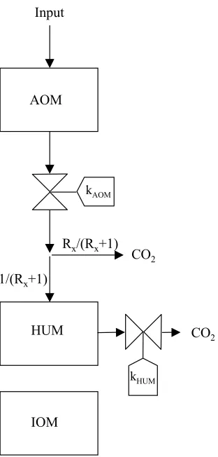
A simple three-pool model is utilised for this demonstration (Fig. 6.1). The
simulations are primarily intended to be heuristic, and the parameters settings are hence not claimed to be universal.
IOM
HUM CO2
CO2
kHUM
1/(Rx+1)
Rx/(Rx+1)
kAOM
[image:19.595.70.226.279.605.2]AOM Input
Figure 6.1. Model structure. Boxes are carbon pools, and valves represent decay rates. Rx depends
on the clay content, and is calculated according to Eq. 12.
6.1. Input file examples
Model structure file: "\c-tool-v1_1\ThreePoolModel\SimpleModel.dat"
[AddedMatter(0)]
Name AOM UseClayEffect 1 DecompositionRate 0.12 Direction(0) HUM Fraction(0) 1.0
[Matter(0)]
Name HUM DecompositionRate 0.0027 Direction(0) CO2 Fraction(0) 1.0
[Matter(1)]
Name IOM
DecompositionRate 0.0 /Totally inert pool
Direction(0) IOM /Although inert, must point at some pool Fraction(0) 1.0 /Fractions must add to one
[Parameters]
WaterResponse 0 /Water response not used ClayResponse 2 /Like Rothc
[end]
The climate file only considers temperature, using monthly averages recorded at the climate station at Askov during 1961-1991.
Microclimate file: "\c-tool-v1_1\ThreePoolModel\climate.dat"
1 1 0.1
8 1 15.7 9 1 12.7 10 1 8.9 11 1 4.4 12 1 1.4
Note that "[end]", which is used to terminate the reading of parameter files, not is used in files with driving variables.
For the examples below, the only type of added organic matter needed to be considered is plant residue. The added organic matter file looks as below
Added organic matter file: "\c-tool-v1_1\ThreePoolModel\addtypes.dat"
[OrganicProduct(0)]
Name PLANTRES
Pool(0) AOM /Only one pool that carbon enters Fraction(0) 1.0
[end]
Three set-ups are considered, each with a separate initialisation file.
1) NPK1 plots. This long-term experiment (Lermarken, sandy loam, B2 field, "NPK1" plots) started in 1894. The experiment is given mineral fertiliser, and employs a four- course crop rotation of winter cereals (wheat and rye), root crops (mangolds, sugar beets, turnips and potatoes), spring cereals (barley and oats) and a clover/grass mixture.
Details of the experiment can be seen in Christensen et al. (1994).
Initialisation file: "\c-tool-v1_1\ThreePoolModel\npk1\initcond.dat"
TotalC 42.2 /t per ha AOM 0.07
HUM 0.53
HUM.PM 99.4 /This pool is of some average C-14 age IOM 0.40 /40% of total carbon assumed to be inert IOM.PM 81.7 /This pool is of substantial average C-14 age ClayContent 0.12 /12 % clay
The corresponding supply file only consists of one line, as all carbon for convenience is assumed to be returned to the soil in August.
Supply file: "\c-tool-v1_1\ThreePoolModel\npk1\added.dat"
8 1 PLANTRES 3.5
An average amount of 3.5 t C ha-1 is assumed to enter the topsoil each year.
2) A purely hypothetical experiment, where a C4-plant (e.g. maize) was assumed to be grown
exclusively since 1950, and to give the same return of C to soil as the C3-plant crop rotation in 1).
Discrimination of 13C occurs in plants, most pronounced in C3 plants. Field trials where C4
plants have replaced C3 plants or vice versa, thus allow for specific tests of model assumptions. The
purpose of this example is to demonstrate the potentials of 13C discrimination for model validation.
Initialisation file: "\c-tool-v1_1\ThreePoolModel\carbon13\initcond.dat"
TotalC 42.2 AOM 0.04 HUM 0.56 IOM 0.40
AOM.d13C -29 /Initial dC-13 in the soil is -29 HUM.d13C -29
IOM.d13C -29 ClayContent 0.12
[end]
Supply file: "\c-tool-v1_1\ThreePoolModel\carbon13\added.dat"
8 1 PLANTRES 3.5 -12
3) Same experiment as 1), but with all incoming carbon being "tagged". Here this is used to assess which fraction of the carbon present at the initiation of the experiment, which was substituted by new matter during the experiment.
The "tagging" option can also be used to analyse internal flow properties, see Petersen et al. (2002).
Initialisation file: "\c-tool-v1_1\ThreePoolModel\tag\initcond.dat"
TotalC 42.2 AOM 0.04 HUM 0.56
IOM 0.40 /All untagged by default ClayContent 0.12
[end]
Supply file: "\c-tool-v1_1\ThreePoolModel\tag\added.dat"
8 1 PLANTRES 3.5 1
The added matter is "tagged"
The control file for the three simulations is seen below:
Control file:"\c-tool-v1_1\ThreePoolModel\setup.dat" [run(0)]
InputDirectory \c-tool-v1_1\ThreePoolModel\npk1\ OutputDirectory \c-tool-v1_1\ThreePoolModel\npk1\ MicroClimateFile climate.dat
SupplyFile added.dat
StructureFile SimpleModel.dat AddTypeFile addtypes.dat ConditionFile initcond.dat DetailFile details.dat StartYear 1894
EndYear 2000 UseAverageAmounts Y UseAverageClimate Y UseRungeKutta Y
IsotopeType 2 /Carbon-14 UsePercentModern Y
[run(1)]
SupplyFile added.dat
StructureFile SimpleModel.dat AddTypeFile addtypes.dat ConditionFile initcond.dat DetailFile details.dat StartYear 1950
EndYear 2000 UseAverageAmounts Y UseAverageClimate Y UseRungeKutta Y
IsotopeType 1 /Carbon-13 [run(2)]
InputDirectory \c-tool-v1_1\ThreePoolModel\tag\ OutputDirectory \c-tool-v1_1\ThreePoolModel\tag\ MicroClimateFile climate.dat
SupplyFile added.dat
StructureFile SimpleModel.dat AddTypeFile addtypes.dat ConditionFile initcond.dat DetailFile details.dat StartYear 1950
EndYear 2000 UseAverageAmounts Y UseAverageClimate Y UseRungeKutta Y IsotopeType 3 /TAG
ReadTAG Y /Read TAG value from addfile [end]
Often the most convenient way to run C-TOOL is from a batch file, placed in the same
directory as the control file "setup.dat". By doing this each group of simulations can have their own directory, with a specimen of the control file. The present simulations were executed via the batch file shown below, which transfers the directory name to the program.
Batch file: "\c-tool-v1_1\ThreePoolModel\c-tool.bat"
6.2. Execution results
The initial state file of example 1) is seen below:
Initial state file: "\c-tool-v1_1\ThreePoolModel\npk1\initstat.txt" Total carbon amount: 42.2
Using average added amounts Using average microclimate StartYear set to 1894 EndYear set to 2000
Fourth order Runge-Kutta integration used Kirschbaum type temperature response used TemperatureAdjust 7.24
Kirschbaum1 -3.432 Kirschbaum2 0.168 KirschbaumTopt 36.9 Water responses not used Carbon-14 simulation Half time 5568 years
Potential clay effect according to RothC-26.3. Value is 4.13 ClayParameter1 3.09
ClayParameter2 2.672 ClayParameter3 -7.86
--- POOL CONTENTS --- Type of pool AddedMatter
Name of pool AOM
Carbon content 2.954 (100 PM) Clay effect is ON
Number of connections 1:
0: HUM. Allocation fraction: 1 Number of sub-pools 1:
Type of pool AOM
Name of pool AOM-subpool Carbon content 2.954
Decomposition rate 0.12 Clay effect is ON Type of pool Matter Name of pool HUM
Carbon content 22.37 (99.4 PM) Decomposition rate 0.0027
Number of connections 1:
0: CO2. Allocation fraction: 1 Type of pool Matter Name of pool IOM
Carbon content 16.88 (81.7 PM) Decomposition rate 0
Number of connections 1:
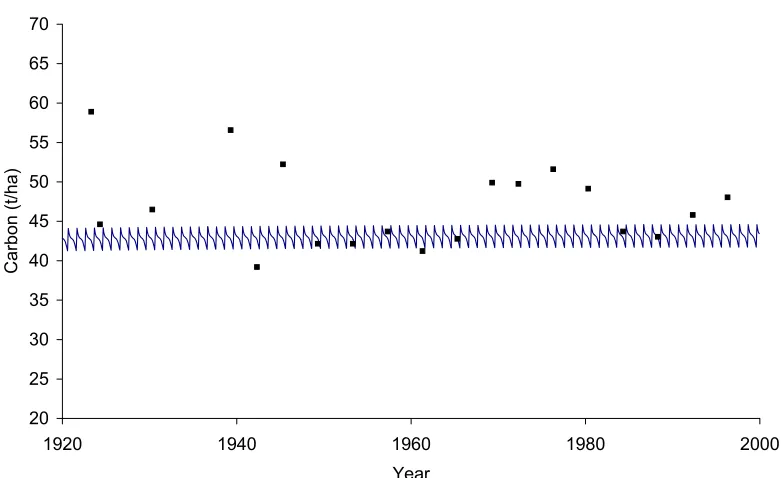
20 25 30 35 40 45 50 55 60 65 70
1920 1940 1960 1980 2000
Year
[image:26.595.72.463.87.326.2]Carbon (t/ha)
Figure 6.2.1. Organic C in soil (0-20 cm) from the Askov Long-term Fertilizer Experiments, Lermarken, B2 field, NPK1 plots, as measured (▪) and modelled (line).
90 92 94 96 98 100 102 104 106
1920 1940 1960 1980 2000
Year
[image:26.595.66.464.429.624.2]pM
Figure 6.2.3. Hypothetical 13C content in soil with carbon input levels as in Fig. 6.2.1, but using C4
plants from 1950.
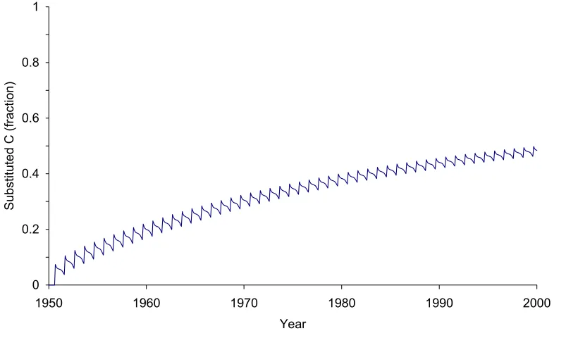
0 0.2 0.4 0.6 0.8 1
1950 1960 1970 1980 1990 2000
Year
Substituted C (fraction)
Figure 6.2.4. Hypothetical "tagged" fraction in soil with carbon input levels as in Fig. 6.2.1. The "tagged" fraction corresponds to the fraction of the original C content that is substituted during the simulation period.
-30 -25 -20 -15
1950 1960 1970 1980 1990 2000
Year
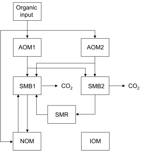
[image:27.595.64.474.444.684.2]7. Execution examples for CN-SIM
The model CN-SIM (Fig. 7.1) and the following simulation examples are taken from Petersen
et al. (2003). All the necessary input files are downloaded together with the program
(www.agrsci.dk/c-tool/). CN-SIM is developed on the basis of a large number of experiments, utilising automated non-linear optimisation for parameter estimation.
Organic input
AOM1 AOM2
NOM IOM
SMB2 CO2
SMB1
SMR
[image:28.595.57.286.233.478.2]CO2
Figure 7.1. Carbon flows in the 7-pool model CN-SIM. AOM1 and AOM2 are added organic matter pools, SMB1 and SMB2 are microbial biomass pools, SMR is a microbial residue pool, NOM is the “humus” pool, and IOM is an inactive pool.
Model structure file: "\c-tool-v1_1\CN-SIM\CN-SIM.dat"
[AddedMatter(0)]
Name AOM1 DecompositionRate 0.122 Direction(0) SMB2 Fraction(0) 0.688 Direction(1) SMB1 Fraction(1) 0.312 [AddedMatter(1)]
Name AOM2 DecompositionRate 1.22 Direction(0) SMB2 Fraction(0) 0.688 Direction(1) SMB1 Fraction(1) 0.312 [BioMatter(0)]
Name SMB1 UseClayEffect 1
UtilizationEfficiency 0.6 DeathRate 0.168 Maintenance 0.194 Direction(0) NOM Fraction(0) 1.0 [BioMatter(1)]
Name SMB2 UseClayEffect 1
UtilizationEfficiency 0.6 DeathRate 2.05 Maintenance 1.84 Direction(0) SMR Fraction(0) 1.0 [Matter(0)]
Name SMR UseClayEffect 1
DecompositionRate 0.134 Direction(0) SMB1 Fraction(0) 1.0 [Matter(1)]
Name NOM DecompositionRate 0.004438 Direction(0) SMB1 Fraction(0) 1.0 [Matter(2)]
Name IOM
DecompositionRate 0.0 /Considered inert Direction(0) IOM
Fraction(0) 1.0 [Parameters]
ClayResponse 3
ClayParameter4 1.67 /Set according to RothC
TemperatureResponse 1 /Kirschbaum temperature response type WaterResponse 2 /Read directly from file
The climate files for Askov consider an “average” water effect, calculated according to Petersen et al. (2003). This effect differs between bare fallow and crop rotation.
For the bare fallow, the climate file is as follows.
Microclimate file: "\c-tool-v1_1\CN-SIM\askov_bares_month.dat"
1 1 0.1 0.96
2 1 0.1 0.96
3 1 2.4 0.96
4 1 6.1 0.96
5 1 10.7 0.96
6 1 13.9 0.96
7 1 15.5 0.96
8 1 15.7 0.96
9 1 12.7 0.96
10 1 8.9 0.96
11 1 4.4 0.96
12 1 1.4 0.96
The climate file for the crop rotation has a slightly lower value for the water effect, due to a higher evapotranspiration.
Microclimate file: "\c-tool-v1_1\CN-SIM\askov_month.dat"
1 1 0.1 0.91
2 1 0.1 0.91
3 1 2.4 0.91
4 1 6.1 0.91
5 1 10.7 0.91
6 1 13.9 0.91
7 1 15.5 0.91
8 1 15.7 0.91
9 1 12.7 0.91
10 1 8.9 0.91
11 1 4.4 0.91
When using CN-SIM on other locations, a water effect value must be determined. When daily climate data are available, this can be done according to Petersen et al. (2003). If daily climate data are not available, and the site is exposed to temperate, humid climate, the above values can be used as proximates for the water effect. If the soil is very light-textured, a value of 0.85 may be more appropriate for vegetated soil (Petersen et al., 2003). This model is only calibrated on agricultural soils with temperate, humid climate, and should only be used with great caution on other types of land use or climate.
For the examples below, two types of added organic matter need to be considered: plant residue and animal manure. The added organic matter file looks as below
Added organic matter file: "\c-tool-v1_1\CN-SIM\addtypes.dat"
[OrganicProduct(0)] Name PLANT Pool(0) AOM1 Fraction(0) 0.45 DecayRate(0) 0.122 Pool(1) AOM2 Fraction(1) 0.55 DecayRate(1) 1.22
[OrganicProduct(1)] Name FYM Pool(0) AOM1 Fraction(0) 0.297 DecayRate(0) 0.091 Pool(1) AOM2 Fraction(1) 0.500 DecayRate(1) 1.22 Pool(2) NOM Fraction(2) 0.203
All five Askov-simulations from Petersen et al. (2003) are considered, each with a separate initialisation file.
1) “ASKOV-FL1-B3”: Fallowed plots from Askov B3 field, including radiocarbon simulation. These plots were kept bare by mechanical weeding during 1956-1985, see (Christensen, 1990) for details.
Initialisation file: "\c-tool-v1_1\CN-SIM\Baresoil_b3\initcond_bares_b3.dat"
TotalC 53.8 /t C per ha ClayContent 0.12 /kg per kg AOM1 0.027
AOM2 0.000 SMB1 0.016 SMB2 0.001 SMR 0.019 NOM 0.532 NOM.PM 99.4 IOM 0.405 IOM.PM 80.5
[end]
Supply file: "\c-tool-v1_1\CN-SIM\soilinp_bares.dat"
4 1 PLANT 0.07 5 1 PLANT 0.10 6 1 PLANT 0.14 7 1 PLANT 0.54
An average amount of 0.85 t C ha-1 is assumed to enter the topsoil each year. The bare soil supply file is common for all three bare fallow simulations.
2) “ASKOV-FL1-B4”: Fallowed plots from Askov B4 field. These plots were kept bare by
mechanical weeding during 1956-1985, see (Christensen, 1990) for details. Supply file shared with 1).
TotalC 49.3 /t C per ha ClayContent 0.12 /kg per kg AOM1 0.027
AOM2 0.000 SMB1 0.016 SMB2 0.001 SMR 0.019 NOM 0.532 IOM 0.405
[end]
3) “ASKOV-FL2”: Fallowed frames from Askov, including radiocarbon simulation. These frames were kept bare by mechanical weeding during 1956-1986, see (Christensen, 1988) for details. Supply file shared with 1).
Initialisation file: "\c-tool-v1_1\CN-SIM\frame_bare\initcond_frame_bares.dat"
TotalC 116.8 /t C per ha ClayContent 0.098 /kg per kg AOM1 0.027
AOM2 0.000 SMB1 0.016 SMB2 0.001 SMR 0.019 NOM 0.532 NOM.PM 99.4 IOM 0.405 IOM.PM 77.4
[end]
4) “ASKOV-NPK”: This long-term experiment (Lermarken, sandy loam, B2 field, "NPK1" plots) started in 1894. The experiment is given mineral fertiliser, and employs a four- course crop rotation of winter cereals (wheat and rye), root crops (mangolds, sugar beets, turnips and potatoes), spring cereals (barley and oats) and a clover/grass mixture.
Details of the experiment can be seen in Christensen et al. (1994).
TotalC 42.2 /t C per ha ClayContent 0.12 /kg per kg AOM1 0.027
AOM2 0.000 SMB1 0.016 SMB2 0.001 SMR 0.019 NOM 0.532 NOM.PM 99.4 IOM 0.405 IOM.PM 78.3
[end]
Supply file: "\c-tool-v1_1\CN-SIM\ NPK1_B2\meaninp_npk1.dat"
4 1 PLANT 0.28 5 1 PLANT 0.42 6 1 PLANT 0.57 7 1 PLANT 2.26
An average amount of 3.53 t C ha-1 is assumed to enter the topsoil each year.
5) “ASKOV-FYM”: This long-term experiment (Lermarken, sandy loam, B2 field, "FYM1" plots) started in 1894. The experiment is given animal manure, and employs a four- course crop rotation of winter cereals (wheat and rye), root crops (mangolds, sugar beets, turnips and potatoes), spring cereals (barley and oats) and a clover/grass mixture.
Details of the experiment can be seen in Christensen et al. (1994).
Initialisation file: "\c-tool-v1_1\CN-SIM\Fym1_b2\initcond_fym1.dat"
TotalC 47.7 /t C per ha ClayContent 0.12 /kg per kg AOM1 0.027
IOM 0.405 IOM.PM 79.4
[end]
Supply file: "\c-tool-v1_1\CN-SIM\ NPK1_B2\meaninp_npk1.dat"
4 1 PLANT 0.25 5 1 PLANT 0.37 6 1 PLANT 0.49 7 1 PLANT 1.97 9 1 FYM 1.0
An average amount of 3.08 t C ha-1 from crop residues and 1.0 t C ha-1 from animal manure is assumed to enter the topsoil each year.
The control file for the five simulations is seen below:
Control file: "\c-tool-v1_1\CN-SIM\setup.dat"
[run(0)]
InputDirectory \c-tool-v1_1\CN-SIM\npk1_b2\ OutputDirectory \c-tool-v1_1\CN-SIM\npk1_b2\ MicroClimateFile askov_month.dat
SupplyFile meaninp_npk1.dat StructureFile CN-SIM.dat
AddTypeFile addtypes.dat ConditionFile initcond_npk1.dat DetailFile details.txt
UseAverageAmounts Y UseAverageClimate Y UseRungeKutta Y StartYear 1953 EndYear 2000 IsotopeType 2 /14C UsePercentModern Y [run(1)]
InputDirectory \c-tool-v1_1\CN-SIM\fym1_b2\ OutputDirectory \c-tool-v1_1\CN-SIM\fym1_b2\ MicroClimateFile askov_month.dat
SupplyFile meaninp_fym1.dat StructureFile CN-SIM.dat
AddTypeFile addtypes.dat ConditionFile initcond_fym1.dat DetailFile details.txt
[run(2)]
InputDirectory \c-tool-v1_1\CN-SIM\BareSoil_b3\ OutputDirectory \c-tool-v1_1\CN-SIM\BareSoil_b3\ MicroClimateFile askov_bares_month.dat
SupplyFile soilinp_bares.dat StructureFile CN-SIM.dat
AddTypeFile addtypes.dat
ConditionFile initcond_bares_b3.dat DetailFile details.txt
UseAverageAmounts Y UseAverageClimate Y UseRungeKutta Y StartYear 1956 EndYear 1985 IsotopeType 2 /14C UsePercentModern Y [run(3)]
InputDirectory \c-tool-v1_1\CN-SIM\BareSoil_b4\ OutputDirectory \c-tool-v1_1\CN-SIM\BareSoil_b4\ MicroClimateFile askov_bares_month.dat
SupplyFile soilinp_bares.dat StructureFile CN-SIM.dat
AddTypeFile addtypes.dat
ConditionFile initcond_bares_b4.dat DetailFile details.txt
UseAverageAmounts Y UseAverageClimate Y UseRungeKutta Y StartYear 1956 EndYear 1985 [run(4)]
InputDirectory \c-tool-v1_1\CN-SIM\frame_bare\ OutputDirectory \c-tool-v1_1\CN-SIM\frame_bare\ MicroClimateFile askov_bares_month.dat
SupplyFile soilinp_bares.dat StructureFile CN-SIM.dat
AddTypeFile addtypes.dat
ConditionFile initcond_frame_bares.dat DetailFile details.txt
UseAverageAmounts Y UseAverageClimate Y UseRungeKutta Y StartYear 1956 EndYear 1987 IsotopeType 2 /14C UsePercentModern Y [end]
The present simulations were executed via the batch file below, which transfers the directory name to the program.
Batch file: "\c-tool-v1_1\CN-SIM\c-tool.bat"
Figure 7.2. Measurements (symbols) and simulations (lines) of soil C and 14C in % modern (0-20 cm depth) from selected treatments from Askov. Askov bare fallow (FL1-B3, ASKOV-FL1-B4 and ASKOV-FL2) are shown left. Data from the crop rotations ASKOV-FYM and ASKOV-MIN are shown right.
1950 1960 1970 1980 1990
pM
C
80 85 90 95 100 105 110
C (t h
a
-1)
0 20 40 60 80 100 120 140
1950 1960 1970 1980 1990 2000
a
b
a b
e d
d
e c
ASKOV-FYM (d) ASKOV-MIN (e) ASKOV-FL1-B3 (b)
8. References
Baxter, M.S. and Walton, A., 1971. Fluctuations of atmospheric carbon-14 during the past century.
Proc. Roy. Soc. London, A. 321: 105-127.
Christensen, B.T., 1988. Effect of cropping system on the soil organic matter content. I. Small plot experiments with incorporation of straw and animal manure, 1956-1986 (in Danish with English summary). Tidsskr. Planteavl92, 295-305.
Christensen, B.T. 1990. Sædskiftets indflydelse på jordens indhold af organisk stof. II. Markforsøg på grov sandblandet lerjord (JB5), 1956-1985 (in Danish with English summary). Tidsskr. Planteavl 94: 161-169.
Christensen, B.T., Petersen, J., Kjellerup, V. and Trentemøller, U. 1994. The Askov Long-Term Experiments on Animal Manure and Mineral Fertilizers: 1894-1994. Minstry of Agriculture. Danish Institute of Plant and Soil Science. SP report no 43.
Coleman, K. and Jenkinson, D.S., 1996. RothC-26.3. A model for the turnover of carbon in soil. In: D.S. Powlson, P. Smith and J.U. Smith (Editors), Evaluation of Soil Organic Matter Models Using Existing, Long-Term Datasets, NATO ASI series I, Vol 38, Springer-Verlag, Heidelberg, pp 237-246.
Hansen, S., Jensen, H.E., Nielsen, N.E. and Svendsen, H., 1990. DAISY – soil plant atmosphere system model. NPo forskning fra Miljøstyrelsen. A10, Miljøministeriet, Copenhagen, 272 pp. Johnsson, H., Bergström, L., Jansson, P.E. and Paustian, K., 1987. Simulation of nitrogen dynamics
and losses in a layered agricultural soil. Agric. Ecosyst. Environ.18: 333-356.
Kirschbaum, M.U.F., 1995. The temperature dependence of soil organic matter decomposition, and the effect of global warming on soil organic C storage. Soil Biol. Biochem. 27: 753-760.
Levin, I. and Kromer, B., 1997. Twenty years of atmospheric 14CO2 observations at Schauinsland
station, Germany. Radiocarbon39: 205-218.
Levin, I., Kromer, B., Schoch-Fischer, H., Bruns, M., Münnich, M., Berdau, D., Vogel, J.C. and
Münnich, K.O. 1994. ∆14C records from sites in Central Europe. In: Boden, T.A., Kaiser, D.P., Sepanski, R.J. and Stoss, F.W. (Editors). Trends ’93: A compendium of Data on Global Change. ORNL/CDIAC-65. Carbon Dioxide Information Analysis Center, Oak Ridge National
Petersen, B.M., Berntsen, J., Hansen, S. and Jensen, L.S. 2003. CN-SIM - a model for the turnover of soil organic matter. I: Long-term carbon and radiocarbon development. Submitted to Soil Biol.
Biochem.
Petersen, B.M., Olesen, J.E. and Heidmann, T. 2002. A flexible tool for simulation of soil carbon turnover. Ecological Modelling151: 1-14.