The North Atlantic heat budget: an Argo based study

Full text

(1)University of Southampton Research Repository ePrints Soton. Copyright © and Moral Rights for this thesis are retained by the author and/or other copyright owners. A copy can be downloaded for personal non-commercial research or study, without prior permission or charge. This thesis cannot be reproduced or quoted extensively from without first obtaining permission in writing from the copyright holder/s. The content must not be changed in any way or sold commercially in any format or medium without the formal permission of the copyright holders.. When referring to this work, full bibliographic details including the author, title, awarding institution and date of the thesis must be given e.g. AUTHOR (year of submission) "Full thesis title", University of Southampton, name of the University School or Department, PhD Thesis, pagination. http://eprints.soton.ac.uk.

(2) UNIVERSITY OF SOUTHAMPTON FACULTY OF ENGINEERING, SCIENCE AND MATHEMATICS School of Ocean and Earth Sciences. The North Atlantic Heat Budget: An Argo Based Study. Thesis for the degree of Doctor of Philosophy by. Rachel Elaine Hadfield. October 2007.

(3) Abstract The Argo dataset is used to obtain estimates of the heat storage and heat divergence with the aim of the assessing the usefulness of the Argo array for investigating the North Atlantic heat budget. The accuracy of the Argo-based mixed layer heat storage varies significantly throughout the North Atlantic. Errors are smallest, around 10-20 Wm-2 on monthly timescales for 10° x 10° boxes, reducing to 5-10 Wm-2 on seasonal scales in the subtropics and eastern basin. Heat storage errors over a fixed 300 m layer are higher, but typically remain below 20 Wm-2 on seasonal timescales away from the western boundary. The heat budget is closed (using net heat fluxes from the NCEP climatology and NOC reanalysis) within the estimated error throughout the subtropical and eastern North Atlantic, indicating the value of the Argo dataset in studies of this nature. However, within the western boundary the heat budget residual typically exceeds 50 Wm-2, with the heat storage overestimated or the heating from the net heat flux and/or advective and diffusive divergence underestimated. Assuming that heat storage error estimates are accurate and considering results in the literature regarding the bias in net heat flux products, it is likely that heating from divergence is underestimated. The heating contribution from this term may be large on scales that cannot be resolved using Argo. In the eastern and subtropical North Atlantic, the errors in the Argo-based heat budget terms are smaller than the uncertainty in the net heat flux products and can thus be used to provide insight into which atmospheric dataset (the NCEP reanalysis or the NOC climatology) may be more accurate. The NOC net heat flux is more accurate than that from NCEP throughout the year in the subtropics and during the first half of the year in the eastern mid-latitudes. The errors in the mixed layer heat storage are smaller than the interannual variability in this term. Thus Argo can be used to investigate variability on this scale. While the current Argo dataset is on the short side for studies of this nature, continued funding of the array is expected to provide more insightful results.. -2-.

(4) Author’s Declaration I Rachel Hadfield, declare that the thesis entitled ‘The North Atlantic Heat Budget: An Argo Based Study’ and the work presented in it are my own. I confirm that - this work was done wholly or mainly while in candidature for a research degree at the University; - where I have consulted the published work of others, this is always clearly attributed; - where I have quoted work from others, the source is always given. With the exception of such quotations, this thesis is entirely my own work; - I have acknowledged all my main sources of help; - parts of this work have been published as Hadfield, et al. (2007).. Signed: ……………………………………………………………………………………….. Date: …………………………………………………….……………………………………. -3-.

(5) Acknowledgements I am very grateful to my supervisors, Dr Neil Wells and Dr Simon Josey, for their help, advice, optimism and encouragement throughout the course of my PhD and to my panel chair, Professor Harry Bryden for his support. I would like to thank Dr Joel Hirschi for his guidance and the many hours he has dedicated to running weekly discussion groups. This opportunity to informally discuss work with other postgraduate researchers has been incredibly helpful. I would also like to thank the members of the Rapid climate change project, in particular Dr Meric Srokosz. The project has funded my PhD and provided several opportunities to present work at annual meetings. These meetings have been interesting and great fun. I am grateful to Dr Elaine McDonagh for making the 36°N data available for use in this study and to Dr Beverly DeCuevas and Dr Andrew Coward for providing OCCAM output. Also many thanks to Dr Steven Alderson for providing access to his Argo-based sea surface height fields and to Dr Josh Willis for sharing his knowledge on the derivation of the velocity field from Argo displacements. This work was supported by the NERC Rapid climate change project, grant no. NER/S/S/2003/11906. The Argo data were collected and made freely available by the International Argo Project and the national programmes that contribute to it (http://www.argo.ucsd.edu, http://argo.jcommops.org). Argo is a pilot programme of the Global Ocean Observing System.. -4-.

(6) Contents AUTHOR’S DECLARATION .........................................................................................3 CONTENTS ......................................................................................................................5 LIST OF TABLES ............................................................................................................7 LIST OF FIGURES ..........................................................................................................8 ACCOMPANYING MATERIAL ..................................................................................11 APPENDICES.................................................................................................................11 ACRONYMS AND ABBREVIATIONS ........................................................................12 CHAPTER 1. INTRODUCTION..................................................................................14 1.1 MOTIVATION ...........................................................................................................14 1.2 AIMS AND OBJECTIVES .............................................................................................16 1.3 THE NORTH ATLANTIC OCEAN: CIRCULATION AND STRUCTURE ................................17 1.4 TEMPORAL VARIABILITY IN THE NORTH ATLANTIC...................................................20 1.4.1 Variability in the North Atlantic Circulation ......................................................................21 1.4.2 Variability in Water Mass Properties..................................................................................23. 1.5 THE HEAT BUDGET ..................................................................................................24 1.6 PREVIOUS ANALYSES OF THE NORTH ATLANTIC HEAT BUDGET ................................25 1.7 REVIEW OF PREVIOUS ARGO-BASED STUDIES ...........................................................28 1.8 STRUCTURE .............................................................................................................31 CHAPTER 2. DATASETS .............................................................................................33 2.1 INTRODUCTION ........................................................................................................33 2.2 ARGO ......................................................................................................................33 2.2.1 Float development.................................................................................................................33 2.2.2 Quality control ......................................................................................................................37 2.2.3 Data distribution...................................................................................................................42. 2.3 ATMOSPHERIC FIELDS FROM CLIMATOLOGY ..............................................................44 2.3.1 Derivation of fields ...............................................................................................................44 2.3.2 The NOC climatology and the NCEP reanalysis................................................................47. 2.4 OCCAM .................................................................................................................50 2.5 THE 2001 WORLD OCEAN DATABASE ......................................................................50 CHAPTER 3. INVESTIGATION OF INTERPOLATION METHODS .....................52 3.1 INTRODUCTION ........................................................................................................52 3.2 STATISTICS OF THE NORTH ATLANTIC TEMPERATURE FIELD ......................................52 3.3 INTERPOLATION METHODS .......................................................................................54 3.3.1 Distance Weighting Schemes ...............................................................................................54 3.3.2 Optimal Interpolation ...........................................................................................................56. 3.4 TESTING INTERPOLATION METHODS .........................................................................57 3.4.1 Simple Averaging schemes ...................................................................................................59 3.4.2 Distance weighting schemes.................................................................................................60. -5-.

(7) 3.4.3 Optimal Interpolation Schemes............................................................................................62. 3.5 SUMMARY ...............................................................................................................69 CHAPTER 4. ACCURACY OF ARGO TEMPERATURE AND HEAT STORAGE FIELDS ...........................................................................................................................70 4.1 INTRODUCTION ........................................................................................................70 4.2 ACCURACY OF AN ARGO DERIVED TEMPERATURE SECTION ......................................70 4.2.1 The Hydrographic Section....................................................................................................71 4.2.2 Cruise and Argo Section Inter-comparison ........................................................................73 4.2.3 Satellite Data Analysis..........................................................................................................78. 4.3 ACCURACY OF ARGO DERIVED HEAT STORAGE ESTIMATES ......................................80 4.3.1 Introduction ...........................................................................................................................80 4.3.2 Estimating the upper ocean heat storage ............................................................................81 4.3.3 Results....................................................................................................................................83. 4.4 THE RELATIONSHIP BETWEEN THE ACCURACY OF ARGO-BASED HEAT STORAGE ESTIMATES AND SAMPLING ............................................................................................86 4.5 MODEL-BASED ERROR ESTIMATION .........................................................................89 4.6 SUMMARY ...............................................................................................................90 CHAPTER 5: THE HEAT BUDGET: TERMS, VARIABLES AND METHODOLOGY .........................................................................................................92 5.1 INTRODUCTION ........................................................................................................92 5.1.2 Applied Sign Convention and Terminology ........................................................................93. 5.2 THE ARGO-BASED MIXED LAYER DEPTH .................................................................94 5.3 THE ARGO-BASED TEMPERATURE FIELD ...................................................................96 5.4 THE HORIZONTAL VELOCITY FIELD ..........................................................................99 5.3.1 The Wind-driven Velocity .....................................................................................................99 5.4.2 The Geostrophic Velocity Field .........................................................................................102. 5.5 THE VERTICAL VELOCITY FIELD ............................................................................109 5.6 THE HEAT BUDGET COMPONENTS ..........................................................................112 5.6.1 The Heat Storage ................................................................................................................112 5.6.2 Entrainment.........................................................................................................................113 5.6.3 The Absorbed Net Heat Flux..............................................................................................114 5.6.4 The Advective Heat Flux Divergence ................................................................................116 5.6.5 Diffusion ..............................................................................................................................117 5.6.6 The Velocity Shear Covariance..........................................................................................118. 5.7 SUMMARY .............................................................................................................119 CHAPTER 6. SEASONAL HEAT BUDGET ANALYSIS .........................................121 6.1 INTRODUCTION ......................................................................................................121 6.2 THE HEAT STORAGE ..............................................................................................121 6.2.1 The mixed layer heat storage .............................................................................................122 6.2.2 The fixed depth heat storage ..............................................................................................125. 6.3 THE NCEP AND NOC FLUXES ...............................................................................128 6.4 THE EKMAN HEAT DIVERGENCE ............................................................................134 6.4.1 The Annual Mean and Seasonal Cycle ..............................................................................134 6.4.2 Sources of Error..................................................................................................................137. 6.5 THE GEOSTROPHIC HEAT DIVERGENCE ..................................................................140 6.6 THE DIFFUSIVE HEAT FLUX....................................................................................141 -6-.

(8) 6.7 THE HEAT BUDGET ................................................................................................143 6.7.1 The Annual Mean Heat Budget of the North Atlantic ......................................................143 6.7.2 The Eastern Subtropical North Atlantic ............................................................................146 6.8.3 Eastern Mid-Latitudes ........................................................................................................147 6.7.4 The Western Boundary Current .........................................................................................149. 6.8 SUMMARY .............................................................................................................151 CHAPTER 7: TEMPORAL CHANGES IN THE NORTH ATLANTIC HEAT BUDGET.......................................................................................................................154 7.1 INTRODUCTION ......................................................................................................154 7.2 INTERANNUAL VARIABILITY IN THE NORTH ATLANTIC HEAT BUDGET ....................154 7.2.1 The Magnitude of Variability in the Heat Budget Components.......................................155 7.2.2 Correlation Between the Heat Budget Components.........................................................156. 7.3 A CASE-STUDY OF INTERANNUAL VARIABILITY .....................................................158 7.4 TRENDS OF TEMPERATURE AND MLD IN THE NORTH ATLANTIC ..............................161 7.5 SUMMARY .............................................................................................................164 CHAPTER 8: DISCUSSION AND CONCLUSIONS .................................................166 8.1 INTRODUCTION ......................................................................................................166 8.2 THE SCALES THAT CAN BE RESOLVED USING ARGO ..............................................166 8.3 THE ACCURACY OF THE ARGO-BASED TEMPERATURE AND HEAT STORAGE FIELDS .167 8.4 HEAT BUDGET CLOSURE ........................................................................................169 8.5 USING ARGO TO INVESTIGATE INTERANNUAL VARIABILITY ....................................171 8.6 CONCLUSION .........................................................................................................173 8.7 FURTHER WORK ....................................................................................................175 APPENDIX 1: DERIVATION OF THE HEAT BUDGET EQUATION...................177 APPENDIX 2: PRESSURE SENSOR ISSUES WITH SOLO FSI FLOATS.............184 REFERENCES .............................................................................................................188. LIST OF TABLES Table 2.1 Quality control statistics for the Argo dataset....................................................38 Table 3.1 RMS temperature differences between the full model temperature field and the subsampled temperature field gridded using different methods. ........................................58 Table 5.1 The maximum penetrative heat flux................................................................115 Table 6.1 Annual mean values of mixed layer heat storage and heat entrainment ...........123 Table 6.2 Annual mean values of fixed depth heat storage with error estimates ..............126 Table 6.3 Annual range in fixed depth heat storage (Wm-2) ...........................................127 -7-.

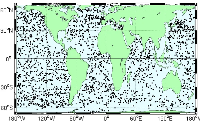
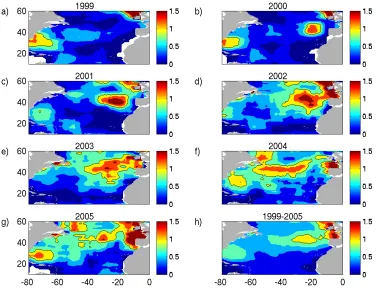
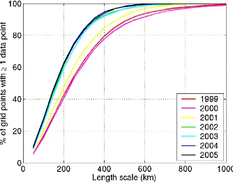
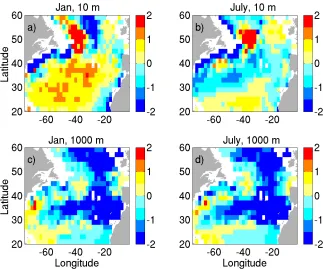
(9) Table 6.4 Annual mean absorbed net heat flux ...............................................................129 Table 6.5 Annual range in absorbed net heat flux ...........................................................133 Table 6.6 Annual mean wind-driven heat divergence ....................................................135 Table 6.7 Mean uncertainty in the seasonal Ekman heat divergence, Wm-2.....................138 Table 6.8 Annual mean geostrophic heat divergence ......................................................140 Table 6.9 The mean diffusive heat divergence................................................................142 Table 6.10 The annual mean heat budget residual...........................................................144 Table 7.1 One standard deviation of the various heat budget components after removal of the mean seasonal cycle ..................................................................................................155. LIST OF FIGURES Figure 1.1 Time series of yearly ocean heat content ........................................................15 Figure 1.2 Components of global energy balance .............................................................15 Figure 1.3 Schematic of the upper North Atlantic circulation . .........................................18 Figure 1.4 Estimates of poleward heat transport in the North Atlantic Ocean. ..................20 Figure 1.5 Sea Level Pressure anomaly (December to March averages) for a) Positive NAO state and b) positive EAP state ................................................................................21 Figure 1.6 Rate of subsurface heat storage change over the upper 300 m in the North Atlantic.............................................................................................................................27 Figure 2.1 The Global Argo float distribution, December 2005 .......................................35 Figure 2.2 Time series of the number of profiles collected by Argo..................................37 Figure 2.3 Example of temperature spikes .......................................................................41 Figure 2.4 Monthly time series of Argo profiles collected in the North Atlantic ..............41 Figure 2.5 Argo sampling density at 10 m for a) 1999, b) 2000, c) 2001, d) 2002, e) 2003, f) 2004, g) 2005 and h) 1999-2005 ...................................................................................43 Figure 2.6 Caption as for Fig. 2.5 but at a depth of 1000 m ..............................................44 Figure 3.1 The percentage of grid points in the North Atlantic that lie within the distances specified on the x-axis and a one month period of at least one data point...........................53. -8-.

(10) Figure 3.2 Difference plot (the interpolation error) between the full model temperature field and the subsampled temperature model field interpolated using a simple averaging scheme..............................................................................................................................59 Figure 3.3 Difference plot (the interpolation error) between the full model temperature field and the subsampled temperature model field interpolated using the Cressman distance weighting scheme .............................................................................................................61 Figure 3.4 OI explanatory figure .....................................................................................64 Figure 3.5 Difference plot between the full model temperature field and the subsampled temperature model field interpolated using an OI scheme with Gaussian covariance, Lx=Ly=100km ..................................................................................................................66 Figure 3.6 Difference plot between the full model temperature field and WOA temperature field . ................................................................................................................................67 Figure 3.7 Difference plot between the full model temperature field and the subsampled temperature model field interpolated using an OI scheme with Gaussian covariance, Lx=Ly=500km .................................................................................................................68 Figure 4.1 The cruise section across 36°N sampled during May and June 2005................72 Figure 4.2 Optimal interpolation statistics across the cruise section .................................72 Figure 4.3 The temperature section across 36°N ..............................................................74 Figure 4.4 Temperature section difference plots w.r.t the hydrographic section................76 Figure 4.5 Depth-averaged differences across the section.................................................77 Figure 4.6 Hovmöller plot (longitude-time) of altimeter SSH anomaly at 36°N................79 Figure 4.7 Annual mean RMS difference between the subsampled and fully sampled OCCAM temperature field estimates of monthly heat storage ..........................................84 Figure 4.8 Time series of mixed layer heat storage HSfull and HSsub .................................85 Figure 4.9 Variation in RMS difference between HSfull and HSsub over the mixed layer, with number of profiles.....................................................................................................87 Figure 4.10 Variations in RMS difference between HSfull and HSsub over the mixed layer, with temporal scale over which the storage is estimated....................................................88 Figure 5.1 Wintertime maximum Mixed Layer Depth (m)................................................94 Figure 5.2 Seasonal cycle in Mixed Layer Depth (m) .......................................................95. -9-.

(11) Figure 5.3 Average temperature (°C) based on seven years of Argo data from 1999 – 2005 at a) 10 m and b) 1000 m. .................................................................................................97 Figure 5.4 Seasonal cycle in Ta and T-h.............................................................................99 Figure 5.5 The wind stress field . ...................................................................................100 Figure 5.6 Vector plot of the velocity field.....................................................................104 Figure 5.7 The Sea Surface Height field from the Bernoulli inverse method (Alderson and Killworth, 2005) .............................................................................................................107 Figure 5.8 Time series of the number of data pairs used to estimate the surface velocity field (black) and the number of data pairs used to estimate the 1000 m velocity..............108 Figure 5.9 Vector plot of the velocity field.....................................................................108 Figure 5.10 Vertical velocity components ......................................................................111 Figure 5.11 Schematic to provide visual explanation of how the April-centred heat storage is calculated from Ta and h..............................................................................................113 Figure 5.12 Schematic to show how temperature gradients are quantified ......................117 Figure 6.1 Seasonal cycle in the total mixed layer heat storage.......................................124 Figure 6.2 Seasonal cycle in the heat storage of the upper 300 m ...................................127 Figure 6.3 Mean absorbed net flux for the NCEP reanalysis and NOC climatology........130 Figure 6.4 Seasonal cycle in absorbed net flux for NCEP and NOC ...............................132 Figure 6.5 Seasonal cycle in heat storage and absorbed net flux .....................................133 Figure 6.6 The mean horizontal Ekman heat divergence ................................................135 Figure 6.7 Seasonal cycle in the horizontal Ekman heat divergence ...............................136 Figure 6.8 Seasonal cycle in the diffusive heat flux ........................................................142 Figure 6.9 Graphical representation of R as given in Table 6. 10. ...................................145 Figure 6.10 The seasonal cycle in the heat budget components at 20-30°N, 35-25°W.....147 Figure 6.11 The seasonal cycle in the heat budget components at 40-50°N, 25-15°W ....148 Figure 6.12 The seasonal cycle in the heat budget components at 30-40°N, 65-55°W.....150 Figure 7.1 Correlation between heat storage anomaly and heat budget components........157 Figure 7.2 Time series of the heat budget components at 20-30°N, 25-15°W. ................159 Figure 7.3 Composite plot of NCEP latent heat flux anomaly and wind stress anomaly vectors for December 2004 ............................................................................................160. - 10 -.

(12) Figure 7.4 Mean temporal trends in a) 10 m temperature, b) 100 m temperature, c) 400 m temperature, d) 1000 m temperature and e) mean temperature between 500 and 1000 m throughout the Argo period, 1999 – 2005, in °C per decade . ..........................................161 Figure 7.5 Temporal trends throughout the water column in a) the eastern subtropical North Atlantic, between 20-30°N, east of 30°W, b) the western subtropical North Atlantic, between 20-30°N, west of 30°W and c) the Labrador Sea ..............................................162 Figure 8.1 a) the warming trend in the mean temperature of the upper 750 m at 50°N, 36°W as measured by Argo and b) projected temperature changes .................................172. ACCOMPANYING MATERIAL A CD containing matlab optimal interpolation programmes, written for use in this study, accompanies this thesis.. APPENDICES APPENDIX 1: Derivation of the heat budget equation. APPENDIX 2: Pressure sensor issues with SOLO FSI floats. - 11 -.

(13) Acronyms and Abbreviations ACCE Atlantic Circulation and Climate Experiment ALACE Autonomous Lagrangian Circulation Explorer C Central subduction buoy CGFZ Charlie Gibbs Fracture Zone COADS Comprehensive Ocean Atmosphere Dataset COARE Coupled Ocean-Atmosphere Response Experiment CTD Conductivity Temperature Depth DACs Data Assemble Centres DMQC Delayed Mode Quality Control DSOW Denmark Strait Overflow Water DWBC Deep Western Boundary Current EAP East Atlantic Pattern ECMWF European Centres for Medium-range Weather Forecast GCM General Circulation Model GDACs Global Data Assembly Centres GFDL Geophysical Fluid Dynamics Laboratory GIN Greenland-Iceland-Norwegian ISOW Iceland-Scotland Overflow Water lNADW lower North Atlantic Deep Water LSW Labrador Sea Water MAR Mid-Atlantic Ridge MBT Mechanical Bathythermograph MLD Mixed Layer Depth MOC Meridional Overturning Circulation MODE Mid-Ocean Dynamics Experiment MOM Modular Ocean Model MW Mediterranean Water NAC North Atlantic Current NADW North Atlantic Deep Water NAO North Atlantic Oscillation NCEP National Centres for Environmental Prediction NCEP/NCAR National Centres for Environmental Prediction/ National Centre for Atmospheric Research NE Northeastern subduction buoy NOC National Oceanography Centre NW Northwestern subduction buoy NWP Numerical Weather Prediction OCCAM Ocean Circulation and Climate Advanced Model OGCM Ocean General Circulation Model OHC Ocean Heat Content OHT Ocean Heat Transport OI Optimal Interpolation RMS Root Mean Square - 12 -.

(14) RTM Radiative Transfer Models RTQC Real Time Quality Control SeaWiFS Sea-viewing Wide Field-of-view Sensor SNR Signal to Noise Ratio SPMW Subpolar Mode Water SSH Sea Surface Height SST Sea Surface Temperature STMW Subtropical Mode Water XBT Expendable Bathythermograph UOR Undulating Ocean Recorder VOS Voluntary Observing Ships WGASF Working Group on Air-Sea Fluxes WMO World Meteorological Organisation WOA World Ocean Atlas WOCE World Ocean Circulation Experiment Table A1 Variables used throughout the thesis Variable g f Ω φ Ta T-h h u, v,. υ w q t ρ Cp HSfull HSsub Av β Ze ^ kx,y kz. Definition Gravity Coriolis force: 2Ωsinφ Earths Rotation Latitude Mixed layer temperature Entrainment temperature Mixed layer depth Eastward and Northward velocity components The horizontal velocity field Vertical velocity field Vertical heat flux Time Density of seawater Specific heat capacity of sea water Heat storage from the model temperature field Heat storage from the subsampled model temperature field Coefficient of turbulent viscosity Latitudinal variation Ekman boundary layer thickness Mean Eddy diffusion coefficient Vertical diffusion coefficient. - 13 -. Value and/or Units 9.8 m2s-1 s-1 Rad s-1 Radians °C °C m ms-1 ms-1 ms-1x,m Wm-2 Seconds 1027 kg m-3 3986 J kg-1 °C-1 Wm-2 Wm-2 m2s-1 m-1s-1 m m2s-1 m2s-1.

(15) CHAPTER 1. Introduction 1.1 Motivation During the 20th century the global climate has shown a considerable warming with a reported increase in the global average sea surface and land surface air temperature of 0.61±0.16 °C (Jones et al., 2001; Folland et al., 2002). The amount of heat stored in the ocean has also steadily increased (Barnett et al, 2005). Levitus et al. (2005) examined the warming signal in global heat content over different depths. Their results, plotted in Fig1.1 indicate that a large part of the observed change in heat content can be accounted for by warming in the upper 700 m. In addition, the global average sea level has risen due to thermal expansion and melting of ice reservoirs at an estimated rate of 1.8±0.1 mm yr-1 from global tide gauge data (Douglas, 1997) or 2.1±1.2 mm yr-1 from altimeter data (Nerem, 1999). These observed changes have important environmental and socialeconomic impacts that cannot be ignored. The recent Stern report on the economics of climate change (October, 2006) and the 4th Assessment of the Intergovernmental Panel on Climate Change provide further evidence for the reality of climate change. To improve our ability to predict future changes, it is necessary to monitor the global climate system and the mechanisms responsible for transporting heat around the globe. The relative importance of the ocean and atmosphere for redistributing heat from low to high latitudes has been the subject of much research (Vonder Haar and Oort, 1973; Oort and Vonder Haar, 1976; Carrisimo et al., 1985; Bryden, 1993; Trenberth and Solomon, 1994; Trenberth and Caron, 2001). Estimates of the ocean and atmosphere heat transports made by Trenberth and Caron (2001) suggest that poleward Ocean Heat Transport (OHT) is dominant only between 0-17°N. However, as shown in Fig. 1.2, atmospheric energy transport and latent heat transport associated with the meridional water transport indicates that the oceans and atmosphere may contribute about equally in maintaining the global heat balance (Bryden and Imawaki, 2001).. - 14 -.

(16) Rachel Hadfield. Chapter 1: Introduction. Figure 1.1 Time series of yearly ocean heat content (1022 J) for the upper 300 and 700m and pentadal (5-year running composites) ocean heat content (1022 J) for the upper 3000 m of the global ocean (Levitus et al., 2005).. Figure 1.2 Components of global energy balance showing the dry static atmosphere heat transport (red), the latent heat transport (green), the ocean heat transport (blue) and the total heat transport (black). Figure created by Bryden and Imawaki (2001) using data from Keith (1995).. - 15 -.

(17) Rachel Hadfield. Chapter 1: Introduction. Investigation of variations in the Ocean Heat Content (OHC), the exchange of heat across the air-sea interface and the OHT can improve understanding of the role of the ocean in the global climate system. Although in principle if two of these terms are known the third can be derived, in practice closure may not be achieved due to observational errors and inaccuracies arising from necessary assumptions made to obtain these terms. Quantification of all three terms is therefore useful for improved understanding of the ocean’s role in climate. 1.2 Aims and objectives The main aim of this thesis is to investigate the accuracy with which the Argo dataset can be used to quantify the seasonal heat storage and heat divergence components of the heat budget. It is anticipated that the Argo dataset may be usefully employed to examine the range, seasonal cycle and the variability in these components. This study is focussed on the North Atlantic Ocean. There are several reasons for this focus. First the relatively high coverage of historical datasets in this region has enabled previous observational analyses of the climatological heat budget. These analyses can be used to help verify results obtained in this study. Second, the North Atlantic plays an important role in maintaining present day global climate through its overturning circulation driven by deep convection and sinking at high latitudes. Thus this ocean basin, with its varied dynamics, provides an ideal opportunity to identify the regions where the Argo dataset can and cannot be used for investigations of the nature outlined above. Third, the North Atlantic OHC is sensitive to changes in global climate (Banks and Wood, 2001) indicating that some interannual variability can be expected in this region. The regions of the North Atlantic where this interannual variability can be captured and studied using the Argo dataset is investigated. Thus the objective of this study is to identify the regions of the North Atlantic where the Argo dataset can be usefully used to further our understanding of the mechanisms responsible for the transfer of heat from the equator to the poles. The upper ocean is of particular interest due to its close coupling with the atmosphere above. Although there are published studies that have investigated the North Atlantic heat budget of the upper ocean (refer to section 1.6 for a review), it is anticipated that use of the Argo dataset in such an - 16 -.

(18) Rachel Hadfield. Chapter 1: Introduction. analysis may be useful for identifying interannual variations in the heat budget components (previous observational analysis on this scale present climatological values only). In addition, this study differs from previous analyses since an attempt is made to quantify each heat budget component individually (rather than inferring any term from knowledge of the others) and careful consideration is given to the errors associated with each heat budget component. In order to accomplish the aims of this thesis it is essential to have an understanding of the study region. To this end, in this introductory chapter a description of the North Atlantic is first given. In the following, the North Atlantic circulation is discussed in section 1.3 and a review of the literature on North Atlantic variability is given in section 1.4. In addition, it is useful to introduce the fundamental equations required for calculating the heat budget terms (section 1.5). Existing heat budget studies are described in section 1.6. A review of studies that use the Argo dataset is given in section 1.7 and the structure of this manuscript is briefly outlined in section 1.8. 1.3 The North Atlantic Ocean: Circulation and structure The large-scale circulation of the North Atlantic Ocean comprises two main components; the horizontal circulation and the vertical Meridional Overturning Circulation (MOC). Although these components of the flow are interlinked, they are described separately here. A schematic of the horizontal circulation in the North Atlantic Ocean is shown in Fig. 1.3. The horizontal circulation is characterized by the presence of two gyres; the anticyclonic subtropical gyre centered on 24°N and the cyclonic subpolar gyre centered around 50°N. The subtropical gyre is bordered to the west by the North American continent until about 36°N, where the Gulf Stream turns east. At the Grand Banks the Gulf Stream splits into 3 sub-branches; one branch recirculating water clockwise, closing the gyre; one continuing east forming the Azores Current and the remainder forming the North Atlantic Current (NAC). The NAC continues as a well-defined boundary current along the eastern slope of the Grand Banks. At about 51°N it divides feeding into the Irminger and Nordic Seas. The current velocities in these branches of the NAC are much lower than in the NAC. - 17 -.

(19) Rachel Hadfield. Chapter 1: Introduction. itself with mean speeds of ~2 cms-1 and 15-20 cms-1, respectively (Tourre et al., 1998). The Labrador, Greenland and Mediterranean basins all exhibit mean cyclonic circulation. The complex topography of the North Atlantic influences the circulation. Exchange between the eastern and western basins of the North Atlantic occurs preferentially over deep gaps in the Mid-Atlantic Ridge (MAR), for example over the Charlie Gibbs Fracture Zone (CGFZ) at ~52°N, the Faraday Fracture Zone at ~50°N and, to a lesser extent, the Maxwell Fracture Zone (~48°N).. Tourre et al. (1998) suggest that this topographic. steering, evident even in near surface flows, may limit the oceans response to climate variations locking cross ridge transports of heat and freshwater to a certain latitude band. This is supported by Cunningham and Alderson (2006), who found changes of opposing sense in the thermocline waters on either side of the MAR.. Figure 1.3 Schematic of the North Atlantic circulation. Red arrows indicate the large-scale surface flow regime, broken arrows indicate deep flow. Contours, with 2.5°C intervals, show the 10 m climatological temperature for June from the World Ocean Atlas. The vertical MOC is driven by the formation of deep-water masses in the Greenland – Iceland - Norwegian (GIN) Seas and the Labrador Sea of the North Atlantic. A study by. - 18 -.

(20) Rachel Hadfield. Chapter 1: Introduction. Pickart et al. (2003) suggested that the Irminger Basin is also a site of deep-water formation, although direct observations have yet to be made. In these deep-water formation regions dense surface waters lose buoyancy through cooling during winter, triggering sinking. Deep-water masses formed in the GIN Seas enter the North Atlantic over sills in the ridge between Greenland and Great Britain (Iceland-Scotland Overflow Water (ISOW)) and the Denmark Strait (Denmark Strait Overflow Water (DSOW)). DSOW and ISOW comprise the bulk of lower North Atlantic Deep Water. DSOW has a cold and relatively fresh signal flowing at depths of more than 3500 m, while ISOW is warmer and saltier and is centred at 2500-3500 m. Water formed in the Labrador Sea (Labrador Sea Water (LSW)) comprises the upper NADW flowing at depths of 1600-2500 m. The estimated 15±2 Sv (1 Sv = 106 m3 s-1) of NADW (Schmitz and McCartney, 1993) is transported south in the Deep Western Boundary Current (DWBC). Other water masses found in the North Atlantic include Mediterranean Water (MW) and Mode Waters. These are typically formed during winter-time by convection. MW is formed in the Mediterranean basin with waters preconditioned for convection through meteorological forcing (Marshall and Schott, 1999). MW, characterized by high salinity and temperature, is found in the North Atlantic at depths of around 1000 m. Mode waters exhibit uniform properties. The main mode waters in the North Atlantic are the Subtropical Mode Waters (STMW) and the Subpolar Mode Waters (SPMW). STMW, commonly referred to as “Eighteen Degree Water” is characterized by temperatures close to 18°C and can be traced throughout the western subtropical gyre at depths of up to 300 m (Marshall et al., 1993). Subpolar Mode Water (SPMW) is found along the branches of the NAC at depths of up to 500 m and is characterized by low potential vorticity (Perez-Brunius et al., 2004). The MOC is responsible for carrying most of the heat transported from the equator to the poles in the North Atlantic Ocean (Roemmich and Wunsch, 1985). Estimates of poleward ocean heat transport in the North Atlantic are shown in Fig. 1.4. Values of 1.2 PW (1 PW = 1015 W), 1.3±0.3 PW, 1.2±0.1 PW, 0.6 ± 0.09 PW and 0.3 PW have been estimated at latitudes of 14°N (Klein et al., (1995), 24°N (Lavin et al., 1998), 36°N (McDonagh, personal comm.), 47°N (Ganachaud and Wunsch, 2003) and 55°N (Bacon, - 19 -.

(21) Rachel Hadfield. Chapter 1: Introduction. 1997), respectively. All estimates given here are derived using hydrographic section data and all contain some element of error.. Figure 1.4 Estimates of poleward heat transport at different latitudes in the North Atlantic Ocean. 1.4 Temporal Variability in the North Atlantic Over the past century, improved ocean monitoring has enabled temporal trends in both the circulation and properties of the North Atlantic to be identified. In this section the literature on these changes is reviewed. Variability in the circulation is discussed in section 1.4.1.. A review of observed temperature changes follows in section 1.4.2.. Before. examining the trends in the North Atlantic, it is instructive to first introduce the leading modes of North Atlantic climate variability, the North Atlantic Oscillation (NAO) and the East Atlantic Pattern (EAP). The anomalous sea level pressure for positive states of the NAO and EAP have been calculated using atmospheric fields from the National Oceanography Centre (NOC) climatology and are shown in Fig.1.5. The NAO is characterised predominantly by cyclical fluctuations of air pressure between the high-pressure system near the Azores and the lowpressure system near Iceland. States of positive NAO exhibit a stronger than normal subtropical high pressure and a deeper than normal Icelandic low. This increased pressure - 20 -.

(22) Rachel Hadfield. Chapter 1: Introduction. difference results in enhanced storm activity and a more northerly storm track. The sealevel pressure pattern associated with the EAP is dominated by anomalously low pressure centred approximately midway between the two centres of the NAO dipole. The EAP is most prominent in winter and non-existent in summer. Both the NAO and EAP have exhibited an upward trend, with the NAO switching to positive values in the 1970s and the EAP switching to positive values slightly later.. Figure 1.5 Sea Level Pressure anomaly (December to March averages) for a) Positive NAO state and b) positive EAP state, based on the NOC climatology pressure field. Anomalies relative to weak NAO and EAP states. Units in mbar.. 1.4.1 Variability in the North Atlantic Circulation Changes in water mass formation and the horizontal gyre circulation have been recorded in the observational record. Curry and McCartney (2001) presented observational evidence for interannual to interdecadal variability in the intensity of the North Atlantic gyre circulation. They found a correlation between observed changes and the state of the NAO, with weakened Gulf Stream and NAC circulation corresponding to periods of low NAO. In addition, a positive correlation between LSW formation and the NAO has been documented. This relationship can be explained by the stronger winds associated with periods of high NAO index and the more north-easterly orientation of the winter storm track. Intense low-pressure centres thus pass over the southern Labrador Sea drawing cold, dry air from the Labrador Continent over the relatively warm surface waters of the sea, driving extreme heat loss and deeper convection. There is a lag of perhaps 2-4 years - 21 -.

(23) Rachel Hadfield. Chapter 1: Introduction. between the atmospheric NAO and LSW thickness, indicative of the ocean’s slower response time (Clarke and Gascard, 1983). Freshwater pulses from the Arctic and the conditions of past winters also influence deep convection and water mass properties (Pickart et al., 2002). In the eastern basin Mediterranean Water plays an influential role in determining water mass properties (Lozier et al., 1995). Due to the difficulty in obtaining direct measurements of the MOC strength, little is known about its variability. Past changes in MOC strength have been investigated using a limited set of observations, while climate models have been used to predict future changes under different global warming and greenhouse gas scenarios. It should be noted that in addition to anthropogenic changes in the MOC, natural multidecadal oscillations in overturning strength have also been modelled (Knight et al. 2005). From observations along a repeat transatlantic section at 24°N the Atlantic MOC appears to have slowed by about 30 % between 1957 and 2004 (Bryden et al., 2005). This result is based on snap-shots of data and may therefore reflect natural variability in the MOC and not a long-term trend. In order to distinguish which of these two possibilities is responsible for changes in the MOC, continuous monitoring of the flow is required. This has only been possible since the inception of the Rapid climate change MOC monitoring array deployed in 2004 (Rapid, 2006). The array consists of 22 moorings across 26°N. Preliminary results from the monitoring array indicate that the natural variability exhibits fluctuations of 5-6 Sv on timescales of less than one year (Kanzow et al., 2007). It is therefore possible that the slow down of the MOC observed by Bryden et al. (2005) is a feature of natural variability. Most General Circulation Model (GCM) projections into the 21st Century show a reduction in the strength of the overturning with increasing concentrations of greenhouse gasses (IPCC, 2001). There is a broad range in the magnitude of this reduction in strength. The MOC in the Geophysical Fluid Dynamics Laboratory (GFDL) GCM showed a complete collapse (Rahmstorf, 1995) while there was no significant change in the MOC in the Max-Plank Institute (MPI) coupled model (Latif et al., 2000). Some models exhibit a partial collapse. For example the Hadley Centre HadCM3 model shows no convection in the Labrador Sea but persistent deep-water formation in the GIN seas (Wood et al., 1999) and the GFDL coupled climate model showed a 40% reduction in the MOC strength - 22 -.

(24) Rachel Hadfield. Chapter 1: Introduction. (Dixon and Lanzante, 1999). This multitude of results highlights our inability to accurately predict how the ocean circulation will be affected by global warming. 1.4.2 Variability in Water Mass Properties Barnett (2005) and Levitus et al. (2005) documented a long-term global mean increase in upper-ocean heat content. Superimposed on this mean trend are shorter periods and smaller regions of warming and cooling. Some of the changes in the North Atlantic are discussed here. In the subtropics (south of 32°N) a general warming trend was observed to persist throughout much of the 20th Century (Roemmich and Wunsch, 1984; Parilla et al., 1994; Bryden et al., 1996; Joyce and Robbins, 1996; Arbic and Owens, 2001; Vargas-Yáñez et al., 2004). This warming was centred at a depth of 600-3000m. Hydrographic data collected from research cruises and the long-term hydrographic station at Bermuda indicate that the warming trend extends back to at least 1922 (Joyce and Robbins, 1996). The rate of warming between 1957 and 1981 at 24°N was 0.08°C per decade (Roemmich and Wunsch, 1984), this slowed to 0.02°C per decade between 1981 and 1992 (Parilla et al., 1994). Hydrographic sections along 52°W and 66°W occupied in 1997 indicated that in the western basin the warming trend has ended with a subsequent cooling observed (Joyce et al., 1999). However, sampling of the eastern part of the 24.5°N section in 2002 revealed that the warming in the eastern Atlantic continued at a higher rate of 0.4°C per decade (Vargas-Yáñez et al., 2004). Below 3000 m, a general cooling trend has been observed at an order of magnitude less than the observed upper ocean warming (Parilla et al., 1994; Arbic and Owens, 2001). In the subpolar North Atlantic, cooling at a rate of ~0.3°C per decade between the 1950s to the late 1980s was documented (Arbic and Owens, 2001). This cooling trend was found to be more pronounced in the west than the east (Read and Gould, 1992). Lazier et al. (2002) and Yashayaev and Clarke (2005) observe a subsequent warming within the Labrador Sea, beginning in the mid-1990s. Joyce et al. (1999) and Koltermann et al. (1999) attribute the observed temperature trends in the subpolar and subtropical regions to changes in LSW properties. A strong negative correlation between the thickness of Labrador Sea Water in its source region and - 23 -.

(25) Rachel Hadfield. Chapter 1: Introduction. temperature anomalies at Bermuda with a time lag of 6 years were found (Joyce and Robbins, 1996). This change in properties is thought to be caused by a combination of changing renewal rates and changing properties of water from which LSW is formed (Read and Gould, 1992). This hypothesis is consistent with the observed increase in salinity on isotherms at a nearly constant rate of 0.010 psu per decade between 1957-1992 in the subtropical gyre (Bryden et al., 1996). In addition to these long-term trends in temperature, significant variability on shorter timescales has also been identified. 1.5 The Heat Budget In this study the form of the heat budget is given in terms of the heat balance equation (Stevenson and Niiler, 1983; Foltz and McPhaden, 2005) with only a brief derivation provided here; refer to Appendix 1 for further details.. The equations governing the. conservation of heat and mass in the upper ocean are ' #T #T * # q "C p ) + $ % &T + w , = ( #t #z + # z. "#$ +. !. !. (1.1a). %w =0 %z. (1.1b). where T is temperature, " horizontal velocity with eastward and northward components u and v, w vertical velocity, q vertical heat flux, "C p the specific heat capacity per unit. ! volume, " # ($!/$x, $ /$y) is the horizontal gradient, x , y and z are the eastward, and t is time. ! northward and vertical ! coordinates respectively !. !. Vertically integrating from depth h to the ! sea surface ! (1.1b) becomes !. ! w"h + v"h # $h = $ # hv a. !. !. (1.2). the subscripts "h and a indicate the variables at depth h and the variables averaged between depth "h and the sea surface, respectively. The vertical velocity at the sea surface is assumed to be equal to zero (rigid lid approximation) and changes in mass due to ! !. ! - 24 -.

(26) Rachel Hadfield. Chapter 1: Introduction. precipitation and evaporation have been neglected. Using (1.1b) and (1.2) and including diffusive heat fluxes, the heat conservation equation (1.1a) vertically integrated from depth. h to the sea surface can be written. !. h. 0 ' "h * "Ta "T Q + Q%h + hv a # $Ta + $ # & vˆTˆdz + (Ta % T%h )) + v%h # $h + w%h , + hk x,y # $ 2Ta + kz,%h = ( "t + "t "z -C p %h. (1.3). !. ) where vˆ is the deviation from the vertically averaged velocity field (v = v a + v ) , Tˆ is the deviation from the vertically averaged temperature T = Ta + Tˆ , kxy the horizonal and. (. ). ! diffusion coefficient, kz,-h the vertical diffusion across the depth surface ! –h, Q the surface ! heat flux and Q"h the penetrative heat flux at depth h . The terms from left to right represent ! the local heat storage, the horizontal advective heat flux, the velocity shear covariance, the ! entrainment and the horizontal and vertical diffusion on the left hand side of the equation. ! ! The entrainment term comprises three components, arising from (left to right) 1) temporal changes in h, 2) horizontal gradients in h and 3) vertical advection. The term on the right hand side is the absorbed net air-sea heat flux. The methods used to quantify each of these heat budget terms are outlined in chapter 5. 1.6 Previous Analyses of the North Atlantic Heat Budget There are many published studies, which have attempted to quantify the North Atlantic heat budget components. The aim here is to provide some details on the datasets used in earlier studies to quantify the heat budget and to briefly summarise their findings. Thus, the limitations of these studies will be revealed, and the need for additional investigation of the role of the oceans in global climate and energy budgets is highlighted. It should be noted here that the change in heat content is referred to, simply as the heat storage. Gabites (1950) carried out one of the earliest studies of the broad-scale mean seasonal heat storage. Due to the lack of subsurface temperature observations at that time, he utilised a sea surface temperature dataset combined with a simplified model of the seasonal - 25 -.

(27) Rachel Hadfield thermocline.. Chapter 1: Introduction. Over the subsequent decades the number and quality of subsurface. temperature soundings steadily increased. Bryan and Schroeder (1960) examined the seasonal heat storage between 20-65°N in the North Atlantic using 20,000 bathythermograph observations.. Some 15 years later Oort and Vonder Haar (1976). (henceforth OV76) examined the seasonal heat storage of the upper 275 m in the Northern Hemisphere oceans using around 400,000 historical hydrographic station soundings and 700,000 bathythermograph casts. Lamb and Bunker (1982) (henceforth LB82) utilised data collected between 70°N and 20°S in the Atlantic, over a period of a decade. This provided 233,957 soundings, enabling quantification of the seasonal heat storage over the upper 300 and 500 m. Air-sea flux climatologies were used alongside the heat storage estimates to infer heat transport divergence as a residual. Hsiung at al. (1989) (henceforth H89) used the Levitus climatology (1982) alongside a naval dataset giving a total of 3.8 million observations. As in LB82, H89 infer heat transport divergence as a residual of the heat storage estimates and the net heat flux. The heat storage results for the upper 275 m of the Northern Hemisphere from OV76 for the upper 300 m from LB82 and H89 exhibit similar seasonal cycles in heat budget components. Values from Lamb and Bunker (1982) are plotted in Fig. 1.6. Each study indicates maximum warming during May to August, maximum cooling in November and December and transitional periods, which generally are close to zero, for March, April, September and October. The largest annual range in heat storage is found at around 4050°N, where maximum summer values are 150-200 Wm-2. Wintertime heat loss is of the same magnitude. Slightly smaller hemispheric heat storage values were found in OV76, than the Atlantic values of LB82 and H89. The inferred heat transport from LB82 and H89 is northwards throughout most of the year in the extratropical North Atlantic (north of 20°N). There is a seasonal cycle, with maximum values in spring (H89). Southwards heat transport is observed in November and December (LB82). The studies discussed above are affected by a spatial sampling bias due to concentration of observations along shipping routes and coastal regions.. Bryan and. Schroeder (1960) observed that some locations in the North Atlantic only had data collected during one or two years and that this could lead to a temporal bias due to decadal changes in OHC. In addition, the accuracy of the XBT dataset is dependent on application - 26 -.

(28) Rachel Hadfield. Chapter 1: Introduction. of corrections to fall rates (Willis et al., 2004). None of the above studies include extensive estimates of the associated errors. However, both OV76 and LB82 suggest a mean standard error in the range 10 – 20 Wm-2. Another limitation of these studies is that only the heat storage and the net heat flux are quantified; the advective and diffusive heat divergence is then inferred from the imbalance of these terms. None of these earlier studies consider interannual variability in heat storage.. Figure 1.6 Subsurface heat storage over the upper 300 m in the North Atlantic. Figure created using data from Lamb and Bunker (1982), Wm-2. Satellite data have been used alongside subsurface observations to try and overcome the spatial and temporal bias inherent in subsurface observational data alone (White and Tai, 1995; Chambers et al., 1997, Willis et al., 2003). Such studies use the correlation between steric height (which can be extracted from altimetric height observations) and subsurface temperature observations to obtain estimates of the subsurface temperature with improved spatial coverage. However, this regression method is of limited accuracy in regions where steric height signals are weak. Guinehut et al. (2004) found that using the regression method on sea surface temperature and altimeter data could explain less than. - 27 -.

(29) Rachel Hadfield. Chapter 1: Introduction. 40% of the signal variance at a depth of 200 m in the North Atlantic subtropical and subpolar gyres. Sarmiento (1986), Böning and Herrmann (1994), Jones and Leach (1999), Wang and Carton (2002), Stammer et al. (2003) and Dong and Kelly (2004) (henceforth DK04) used Ocean General Circulation Models (OGCMs) to investigate the components of the North Atlantic heat budget. These studies indicate a primary balance between the net surface heat flux and local storage in the mid-latitude oceans.. In addition, DK04 noted that the. contribution of advection and diffusion to the mixed layer temperature tendency can be significant spatially and temporally. Results from Böning and Herrman (1994) and DK04 are consistent with the observational studies of LB82 and H89, exhibiting a seasonal cycle in poleward heat transport, with maximum values in spring and summer. Results from Wang and Carton (2002) are in contention with minimum heat transport in January – June. However, these latter results are based on an analysis of the full ocean depth. DK04 also investigated the interannual variability in heat storage, with a focus on the Gulf Stream region of the North Atlantic. Their results indicated that interannual variations in the mixed layer temperature are dominated anomalous advection. Results from these studies are dependent on the observational data assimilated into the model and application of accurate ocean physics in the applied models. To date, only a few studies have utilised the Argo subsurface temperature dataset (chapter 2) to examine the heat storage of the North Atlantic.. Lavender (2001) and. Centurioni and Gould (2004) used float data to quantify heat storage in the Labrador and Irminger Seas, respectively. Willis et al. (2004) used float data alongside XBT and altimeter data to quantify OHC on a global scale. Although Willis et al. (2004) examined variability in OHC between 1993-2003, they did not give a break down into different ocean basins and none of the studies considered the annual cycle in OHC. More details on Argobased studies follow in the review in section 1.7. 1.7 Review of Previous Argo-Based Studies More than 170 papers and reports based on data collected by autonomous floats have been written in the past seven years, many appearing in peer-reviewed journals. These studies cover a broad range of purposes, including investigation of sea surface height fields, salinity structure, mixed layer depth, subsurface circulation and oxygen concentration. Only - 28 -.

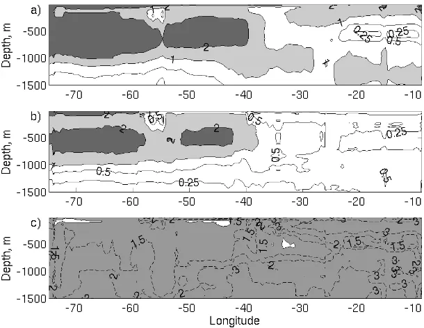
(30) Rachel Hadfield. Chapter 1: Introduction. studies that use float data to quantify changing ocean temperatures and heat content are discussed here. For a full list of published studies based on autonomous drifter data refer to the Argo website (2006). For the past 3 years, the Argo project, discussed in detail in chapter 2, has provided the largest single source of subsurface temperature data in the global oceans. As such it is valuable for quantifying the oceans role in the climate system, through investigation of changing ocean temperatures. There are several existing studies in the literature that use Argo data, both independently and alongside additional datasets, to this end. Willis et al. (2004) published the earliest study of this nature. In their study, data from profiling floats was combined with other historically available subsurface temperature data and satellite altimetric height fields using the method of Willis et al. (2003). A global warming in the upper 750 m during 1993 – 2003 was observed at an average rate of 0.86 ± 0.12 Wm-2. Levitus et al. (2005) used Argo data alongside additional historical temperature data collected using Expendable BathyThermographs (XBTs), shipboard Conductivity Temperature Depth (CTDs) and moored buoys to calculate the heat content over a deeper depth (0 – 3000 m) and over a longer time period, spanning 1955 – 2003. They observed an average warming rate of 0.2 Wm-2 over this period. Gille (2002) used data from floats deployed during the World Ocean Circulation Experiment (WOCE) to examine heat content changes in the Southern Ocean. These early floats did not record temperature profiles during ascent but do provide temperature data from the drift depth, which ranged from 700 to 1100 m. The float temperature records, which provide data throughout the 1990s, were compared to earlier hydrographic temperature measurements from the region. Gille reported an increase in Southern Ocean mid-depth temperatures by around 0.17 °C between the 1950s and the 1980s. While the studies discussed above incorporate data from autonomous drifters, they are not exclusively based upon it. On the contrary a large proportion of the time periods considered in these studies predate the Argo project. In addition, the depth over which heat content is quantified in Levitus (2005) extends below the depth of Argo float profiles. There are several studies in the literature that rely solely on Argo data to quantify changes in subsurface temperature and heat content. Such studies typically focus on select regions of the World Ocean. The earliest studies of this nature investigated the subpolar oceans - 29 -.

(31) Rachel Hadfield. Chapter 1: Introduction. (Lavender, 2001; Centurioni and Gould, 2004; Wirts and Johnson, 2005). WOCE float deployments were typically concentrated in such regions to exploit the unique resource of wintertime hydrographic observations provided by autonomous drifters. Lavender (2001) examined the general circulation and temperature and salinity variability in the Labrador Sea using more than 200 floats deployed between 1994 and 1998.. The hydrographic data was used to investigate deep convection and the one. dimensional heat budget during the winter of 1996-97 and 1997-98. Changing subsurface temperatures were investigated in the Irminger basin using 7725 profiles taken between November 1994 and June 2003 (Centurioni and Gould, 2004). A general warming trend was evident with temperatures of 2.85 ± 0.1 °C in 1997 rising to 3.07 ± 0.08°C in 2003. Wirts and Johnson (2005) observed a warming trend in the southeast Bering Sea using data collected between May 2001 and October 2004. The warming was reported to be of the order 1°C between May 2001 and September 2003. A slight cooling was also observed during the winter of 2003/2004, although this was entirely reversed by warming near the end of the record. More recent studies on subsurface temperature changes inferred exclusively from Argo data have focussed on the North Atlantic (Ivchenko et al., 2006) and the sea south east of Japan (Yoshida and Hoshimoto, 2006). Ivchenko et al. (2006) estimated the heat content anomaly over different layers in the upper 1500 m using profile data obtained from autonomous floats between January 1999 and December 2005. Over 400 profiles per month were used in this analysis. An average warming over the upper 1500 m during the study period at a rate of 0.88 Wm-2 was observed. Despite this general warming, periods and regions of cooling were identified. In particular, cooling occurred at low latitudes after 2003 and throughout the North Atlantic in the 1000 – 1500 m layer. Ivchenko’s dataset includes some Argo floats with pressure sensor problems (Appendix 2), thus some of the observed trends may be spurious. The heat content change in a warm core ring in the sea east of Japan was investigated using 90 profiles obtained from one Argo float (Yoshida and Hoshimoto, 2006). Surface heat flux values were found to be consistent with changes in the heat content in the surface isothermal layer. In addition to studies based on quantifying temporal changes in subsurface temperature, the Argo dataset has been used to investigate the potential temperature – - 30 -.

(32) Rachel Hadfield. Chapter 1: Introduction. salinity (θ-S) relationship (King and McDonagh, 2005; Johnson, 2006), the upper ocean temperature structure (Molinari, 2004) and seasonal and interannual variations in heat transport (Straneo, 2006). King and McDonagh (2005) used data from 30 floats in the vicinity of 32°S in the Indian Ocean to examine changes in the θ-S relationship of the Subantarctic mode water. Relative to shipboard CTD data sampled in 1987 the salinity was observed to increase on temperature levels, consistent with findings from shipboard CTD data sampled in 2002. Changes in θ-S have also been investigated over shorter time periods using Argo data. For example, an isopycnal potential temperature-salinity anomaly in the South Pacific was investigated using 2 profiling floats in austral winter 2004 (Johnson, 2006). The anomaly had a signal of more than 0.35 psu in salinity and 0.9 °C in temperature. Molinari (2004) examined the temperature structure of the upper 750 m in the north western subtropical North Atlantic using data collected between 1950-2003. Most of the data consists of bathythermograph readings, but some float profiling data is included during the period 1998-2001. It was found that the interannual variability in the position of the 18° isotherm observed with XBT data could be reproduced using float data (Molinari, 2004). Straneo (2006) examined the variations in heat and freshwater transport through the central Labrador Sea using profiling float data from 1996 to 2000 and data collected by the Ocean Weather Station Bravo between 1964 and 1974. The float dataset consisted of more than 800 float profiles. Heat divergence was found to have increased between the two periods considered. 1.8 Structure Here a short description of the structure of this manuscript is given. In this thesis the Argo dataset, which is used to investigate the North Atlantic heat budget is introduced in chapter 2. Suitable interpolation methods and lengths are explored in chapter 3. In chapter 4, an analysis of the accuracy of the Argo-based temperature and heat storage fields is carried out. In chapter 5, the variables used to obtain estimates of the different heat budget components are quantified providing essential grounding for the heat budget analysis. The seasonal cycle in individual heat budget components is presented in chapter 6 and the closure obtained is discussed. Interannual variability is investigated in chapter 7. The aim. - 31 -.

(33) Rachel Hadfield. Chapter 1: Introduction. here is to provide insight into the mechanisms responsible for recent observed changes in the North Atlantic temperature field and to yield further understanding of the limitations and capabilities of current atmospheric and oceanic observing systems.. - 32 -.

(34) CHAPTER 2. Datasets 2.1 Introduction In the research described here a variety of datasets and model outputs are exploited to investigate the North Atlantic heat budget. In particular subsurface temperature and drift datasets from the Argo program and atmospheric variables from the National Centers for Environmental Prediction/National Center for Atmospheric Research (hereafter referred to as NCEP) reanalysis and the National Oceanography Centre (NOC) climatology are used to quantify the heat budget components. An Ocean General Circulation Model (OGCM), the Ocean Circulation and Climate Advanced Model (OCCAM) is used to examine the validity of assumptions made and to estimate errors in the heat budget terms (Chapter 4). The 2001 World Ocean Atlas (WOA) monthly climatological temperature field provides a first-guess during interpolation of the Argo temperature data (Chapter 3). In addition, the WOA salinity field is used in calculations of potential temperature and geostrophic velocity. In this chapter these different datasets are discussed starting with the Argo dataset in section 2.2. The atmospheric datasets are described in section 2.3. Section 2.4 gives details on the OCCAM model and in section 2.5 derivation of the WOA temperature and salinity fields is briefly outlined. 2.2 Argo The International Argo program, which began in 1998, aims to deploy a global array of 3000 profiling floats to monitor the state of ocean temperature and salinity.. The. technological development of the Argo floats is outlined in the first sub-section. Quality control procedures are described in section 2.2.2 and in section 2.2.3, the Argo sampling density is discussed. 2.2.1 Float development The earliest neutrally buoyant floats invented in 1955 were developed to investigate subsurface circulation (Swallow, 1955; Swallow, 1957). Tracking involved the use of a dual hydrophone array to determine the floats azimuth relative to the ship. Despite success - 33 -.

(35) Rachel Hadfield. Chapter 2: Datasets. with the Aries experiment, in which Henry Stommel’s model for deep circulation was verified (Swallow, 1971), the 6 km tracking range limited the utility of these early floats. However, during the late 1960’s long-range tracking using the SOFAR channel and moored sound receivers (Rossby and Webb, 1970) rectified this issue and enabled systematic exploration of mesoscale features over a substantial part of the ocean basin, paving the way for the 1973 Mid-Ocean Dynamics Experiment (MODE) (MODE Group, 1978). In the subsequent generation of floats, the transmitter and receiver positions were reversed so that the floats listened to moored sound sources (Rossby et al., 1983). Data was then transmitted through the Argos Satellite System at the end of the mission. The first autonomous (i.e. not requiring an acoustic tracking network) float was the Autonomous Lagrangian Circulation Explorer (ALACE). ALACE floats were developed in the late 1980s and tested in the Drake Passage in the early 1990’s (Davis et al., 1992). The ALACE float cycles from the surface to pre-programmed depths with buoyancy changes accomplished by moving hydraulic fluid between an internal reservoir and external bladder. These floats relay their position to the Argos Satellite System upon surfacing, thus discarding the need for communications with underwater transmitters or receivers. During WOCE in the 1990s, ALACE floats were fitted with temperature, and later, salinity sensors in order for profiles to be taken during ascent and these were called Profiling ALACE, or PALACE floats. Based on the experience in WOCE, in 1998 a plan was presented to develop a global array of profiling floats on a 3° grid throughout the ice-free areas of the deep ocean. It was anticipated that these floats would provide measurements of subsurface currents, temperature and salinity. The float plan, called Argo, is a multinational collaboration with 27 countries involved. The first Argo floats were deployed in late 1999 and over the past 7 years there has been a steady increase in the number of active floats. Since mid 2003 Argo has been the largest single source of ocean profiling data, collecting more profiles than the previous largest source, XBTs. As well as being more numerous, the Argo data go deeper than the 750 m XBTs, measure temperature more accurately and also provide conductivity, enabling determination of salinity and density, and ocean current data. The status of the array in December 2005 is shown in Fig. 2.1. At this time there were 2090 active floats in - 34 -.

(36) Rachel Hadfield. Chapter 2: Datasets. the World Ocean. Note that by March 2007, this figure had reached more than 2800. The floats have a design life of around 4 years requiring that 800 floats are deployed per year to maintain the 3° x 3° array of 3000 floats. The floats deployed by the Argo program typically drift at a depth of 1000 m and profile to 2000 m every ten days.. Figure 2.1 The Global Argo float distribution, December 2005 showing 2090 active floats. The accuracy of float temperature readings is ± 0.005 °C in the early float models (Davis et al., 2001), improving to ±0.002 °C for the later models (Oka, 2005). Similarly, the accuracy of the pressure readings varies among models and is subject to a hysteresis error of ±2 to ± 5 dbar. Salinity data are generally accurate to ± 0.01 psu. Typically the drift in the pressure and temperature is assumed to be negligible, while the conductivity sensor is vulnerable to biofouling, causing long-term salinity drifts (Davis, 1998). Oka (2005) recovered three profiling floats after 2 – 2.5 years of operation and recalibrated their sensors to determine the temperature, pressure and salinity offsets. The temperature drift for the recovered floats varied between +0.001 to +0.002 °C which is within the precision of the calibration. However, both the pressure and salinity exhibited significant drifts of +5.92 ± 0.93 dbar and -0.0125 psu respectively. The surface pressure recorded by the float revealed a jump of a few dbar after the first dive and a gradual drift - 35 -.

No results found